Optical and Numerical Investigations on Combustion and OH Radical Behavior Inside an Optical Engine Operating in LTC Combustion Mode

Abstract

Low Temperature Combustion (LTC) is a relevant process for internal combustion engines (ICE). This combustion mode is based on premixed fuel/air and fuel lean in-cylinder mixture allowing reduction in NOx and PM emissions while maintaining higher thermal efficiency. In order to investigate the effect of engine operating conditions on the behavior of LTC mode, including OH radical evolution, optical measurements and numerical simulations were performed on a transparent CR diesel engine. The homogeneity of the engine charge was obtained by using very early injection timings. In this study, varying injection strategies were investigated for different engine speeds. In parallel to the experimentation, simulations of LTC mode for the same experimental operations were carried out. The model used in this study is based on a stochastic reactor model. This model includes a turbulence (k-ε) model based on a zero-dimensional energy cascade to calculate the turbulent time scale during the cycle. On the other hand, due to the stochastic approach and to reduce initial heterogeneities of the mixture, a confidence parameter was introduced in the global model to consider the real variation ranges of engine. This latter was modeled as a function of the Reynolds number allowing to initiate heterogeneities of temperature and of species mass. OH radicals were estimated with high spatial and temporal resolution using chemiluminescence measurements. Simulated in-cylinder pressure and the OH radical rate were compared to the experimental data. A good agreement was observed in terms of in-cylinder pressure trace and ignition delay times, meaning that the confidence coefficient model is accurate to describe the initial heterogeneities of the mixture. The simulated OH rate profile has the same shape as the measured OH trace and the main ignition occurs at the same time. This study corroborates that the OH radical is an appropriate tool to identify combustion stages.

1. Introduction

Electrification of transport, together with the decarbonization of energy production are suggested by the European Union for the future quality of air and in response to the demands of younger-generation opinion movements. Nevertheless, in the medium period, propulsion systems will continue to dominate urban mobility, making mandatory the retrofitting of thermal engines by applying combustion modes able to reduce NOx and PM emissions while maintaining engine performances. Low Temperature Combustion (LTC) is an attractive process to meet this target. This combustion mode is based on premixed fuel/air and fuel lean in-cylinder charge, allowing low NOx and PM emissions due mostly to its low local combustion temperature. The LTC process can be achieved by various modes, such as: Homogeneous Charge Compression ignition (HCCI), Premixed Charge Compression Ignition (PCCI), and Reactivity Controlled Compression (RCCI). Reference [1] gives a complete review of these combustion modes. The present study focuses on HCCI process which is one of the promising low temperature combustion (LTC) processes [2,3].

In the case of LTC and/or HCCI processes, the in-cylinder charge is perfectly homogeneous, leading to no significant effect on turbulence. However, this ideal homogeneity is not reached in real engines, whatever the type of injection strategy: port or direct. The experimental published papers [4,5,6] have shown that inhomogeneities of temperature and of fuel concentration are highlighted in the combustion chamber. Consequently, the turbulence has a large effect [7,8,9] on: the combustion duration, the ignition delay time, and the pollutant formation processes. Hence, an accurate model to describe the turbulence mixing and the interaction of turbulence with chemistry is required for the LTC process. Transported probability density function (PDF) approaches seem more suitable to model the effects of turbulent mixing and mixture stratification [10,11,12,13,14,15], especially for the LTC combustion mode. As a reminder, simulation is key to support an understanding of complex physical phenomena such as the LTC process, in order to reduce the use of expensive prototypes and time-consuming testing activities. This is the main motivation for the overall project focusing on LTC modeling.

In previous studies [16,17], the micro-mixing has been described through an IEM (Interaction by Exchange with the Mean) model. The main advantages of IEM model are its simplicity and its short computational time. This stochastic approach works on the principle that the mixture in the combustion chamber is represented by a certain number of computational particles. Each particle evolution is due to the rate of change in the chemical reaction term and the mixing term. The chemical reaction term has been modeled with a reduced n-heptane oxidation mechanism developed previously [18], including 25 species and 26 elementary chemical reactions. Note that this reduced mechanism is able to describe accurately the ignition delay times and the rate of heat release. The main objective of these preliminary studies was directed to the optimization of computational time at varying stochastic particle number for three distributions: normal, lognormal, and hat. The numerous results point out that the hat distribution is not accurate for LTC combustion and that a particle number equal to 200 is a good trade-off between the accuracy of the solution and the computation time [16]. In addition, the above-mentioned studies have shown that the turbulent time scale introduced by the IEM model requires physical description instead of a fixed value parameter. Moreover, to further reduce the computation time, random initial distribution was restricted via a fixed parameter [17]. This latter also has an important effect on the solution.

The modeling approach has been further developed by the description of the turbulent time scale through a (k-ε) model based on zero-dimensional energy cascade [19]. This step allows to build an autonomous model with varying turbulent time scale during the cycle. The results of the model have been validated against two engine operating conditions with a single early injection in the cycle. In reference [20], further validation of the time scale model against experimental data has been carried out, when the engine operates with five early injection in the cycle at 1000 rpm engine speed. This study has confirmed that a variable time scale is more accurate than a fixed one.

The goal of the present study is numerical and experimental analysis of LTC (i.e., HCCI) combustion. Experimentally, optical DI diesel engine with high injection pressure system was used to investigate HCCI behavior under various injection strategy and engine speed. In order to obtain a mixture close to homogeneous, very early injection timings were used to ensure sufficient time for mixture preparation. Two injection strategies were used based on five early injections per cycle and four early injections per cycle. Combined measurements were used in order to catch information about the in-cylinder HCCI combustion evolution. OH radical was estimated with high spatial and temporal resolution using chemiluminescence measurements. Moreover, flame emission spectra from UV to visible allowed to evaluate, with more details, in-cylinder OH radical during the main ignition of the combustion period. This radical represents a good indicator of the main ignition timing [18] when the peak of reaction rate is attained.

Numerically, the previous IEM model [19] including the turbulence model was used in the present study. The goal here is to validate the confidence coefficient expressed as a function of Reynolds number and OH radical behavior. OH radical was simulated by the previous semi-detailed n-heptane kinetic mechanism containing 37 species and 61 elementary chemical reactions [18] and compared to experimental results. Note that this reduced mechanism is more accurate to simulate species evolutions compared to the reduced n-heptane mechanism with 25 species and 26 elementary chemical reactions used in the previous studies [16,17,19]. On another hand, the confidence coefficient allowing the restriction of random initial distribution describes the initial heterogeneities amplitude of temperature and of species mass in the combustion. This coefficient introduced in this modeling approach is extremely dependent on engine operating conditions and in-cylinder aerodynamics.

The engine configuration and experimental procedures used in this study are presented in the next section. The global model is presented in the second section. This section includes a summary of the stochastic reactor model, the key equations of the turbulence model and the presentation of the confidence coefficient modeling methodology. The third section deals with the experimental and numerical results, including the comparison and discussion of numerical results against experimental data. The last section presents the conclusion.

2. Engine Configuration and Experimental Procedures

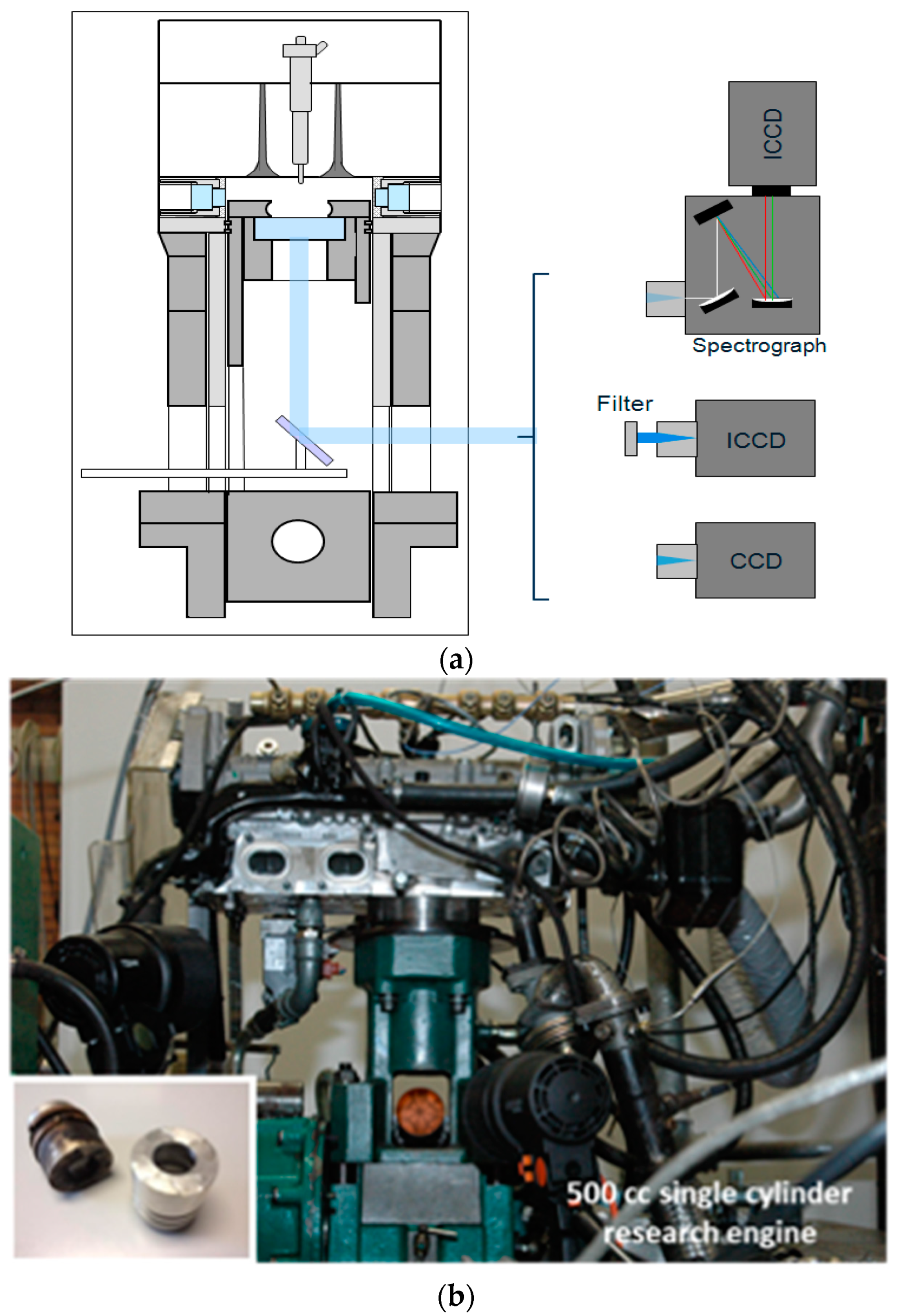
2.1. Research Engine

A single cylinder research engine was used (Figure 1). The engine head was from a direct injection, four-stroke, diesel production engine (Figure 1b).

Table 1. Engine specifications.

Bore [cm]	8.5
Stroke [cm]	9.2
Compression ratio	17.7:1
Bowl volume [cm3]	18.4
Displacement [cm3]	522

reports specifications of the engine. Particular attention was devoted to the management of the water-cooling and lubricating oil. The optically accessible engine is designed with extended piston and piston crown window of 46 mm diameter (Figure 1a). Temperature and pressure of the air at the intake manifold was controlled. Moreover, the Common Rail (CR) injection system managed the diesel fuel directly injected in the bowl by a solenoid injector with 7-hole nozzle. A pressure regulator located on the high-pressure pump ruled the injection pressure; and the ECU governed the number of injections (up to 5) per cycle, the start, and the duration of the injections. A Hall-effect sensor was adopted to monitor the injection signals and a piezoelectric pressure transducer was set in the glow plug seat of the engine head to measure the in-cylinder combustion pressure [6]. Two hundred in-cylinder combustion cycles were recorded via data acquisition system and elaborated to determine the rate of heat release curves [21].

2.2. Engine Operating Conditions

Three engine speeds of 1000 rpm, 1500 rpm, and 2000 rpm were set for this study. On another hand, two injections strategies were carried out during the compression stroke [22]: one with four injections and the other one with five injections. Quasi-homogeneity of the in-cylinder charge for HCCI combustions was guaranteed with early injection timings. The injection had very short duration in order to reduce the spray wall impingement. The investigated strategies are reported in

Table 2. Engine operating conditions when the engine speed is fixed at 1000, 1500, and 2000 rpm.

Engine Speed [rpm]	1000			1500				2000
Injection pressure [bar]	700	900	1000	400	500	600	700	400	500	600	700
Energizing time [μs]	400	350	320	470	440	410	390	450	420	370	350
SOIpilot [CAD]	−70	−70	−70	−55	−55	−55	−55	−70	−70	−70	−70
SOIpre [CAD]	−60	−60	−60	−45	−45	−45	−45	−55	−55	−55	−55
SOImain [CAD]	−50	−50	−50	−35	−35	−35	−35	−45	−45	−45	−45
SOIafter [CAD]	−40	−40	−40	−25	−25	−25	−25	−30	−30	−30	−30
SOIpost [CAD]	−30	−30	−30	-	-	-	-	-	-	-	-

: five injections per cycle and four injections per cycle was realized at 1000 rpm and 1500 rpm as well as 2000 rpm, respectively. To deliver the same diesel amount within the cylinder, the injection pressure (Prail, Canberra, Australia) and energizing time (ET) were varied, increasing the pressure, the latter decreasing. At fixed injection pressure, all the injections had the same duration called energizing time.

2.3. Optical Apparatus

Imaging and chemiluminescence measurements from ultraviolet (UV) to visible were performed by means of the optical set up, in order to catch information about the in-cylinder HCCI combustion evolution [23]. As already reported in other papers [6], two cameras were used to detect images from the combustion within the cylinder. In particular, combustion flames were recorded by the cameras through the piston crown window and a 45° mirror, placed in the elongated piston. The intensified CCD camera (ICCD) oversaw the acquisition of images from UV to near visible, while the second CCD was more sensible in the visible wavelength range. Moreover, a 310 nm bandpass filter was set in front of the ICCD camera lens. It permitted to select and analyze the in-cylinder emission at 310 nm that is characteristic of the OH emission (details of measurements procedure are given in previous paper [6]). It is a characteristic radical due to the autoignition of the premixed charge. A delay unit linked with the engine shaft encoder allowed the synchronization of the two cameras with the in-cylinder combustion phase. This optical layout allowed studying the in-cylinder HCCI combustion evolution in terms of spatial distribution and temporal evolution of radical and flames. Images were acquired from separate combustion cycles and the more representative were selected and reported [6,23].

3. Model Description

3.1. In-Cylinder Model

The Partially Stirred Reactor (PaSR) model is based on statistical homogeneity of the mixture and represents a good tool to investigate the interaction of turbulence and chemistry. For particle methods dedicated to combustion process, the PaSR model is adapted to take into account the large coupled reaction mechanism and mixing process [10,24]. Accordingly, in this study a stochastic reactor model based on the PaSR was used to model LTC combustion mode. The engine cycle used in this approach includes compression and expansion strokes in the combustion chamber (compression, combustion, and expansion). By using PDF transport equations assuming statistical homogeneity, the stochastic reactor model is written as:

$$\frac{\partial F\left(\mathsf{\psi },\mathrm{t}\right)}{\partial \mathrm{t}}-{\displaystyle \sum }_{\mathrm{i}=1}^{\mathrm{s}+1}\frac{\partial }{\partial {\mathsf{\psi }}_{\mathrm{i}}}\left[({\mathrm{H}}_{\mathrm{i}}\left(\mathsf{\psi }\right)+\mathrm{C}{\mathsf{\varphi }}_{\mathrm{i}}\left(F\left(\mathrm{t}\right),\mathsf{\psi }\left(\mathrm{t}\right)\right)F\left(\mathsf{\psi },\mathrm{t}\right)\right]=0$$

(1)

The stochastic process $\mathsf{\psi }\left(\mathrm{t}\right)$ corresponding to the solution $F\left(\mathsf{\psi },\mathrm{t}\right)$ of Equation (1) is determined by the system of ordinary differential equations:

$$\frac{{\mathrm{d}\mathsf{\psi }}_{\mathrm{i}}\left(\mathrm{t}\right)}{\mathrm{dt}}=-{ \mathrm{H}}_{\mathrm{i}}\left({\mathsf{\psi }}_{\mathrm{i}}\left(\mathrm{t}\right)\right)-\frac{C}{\tau }\left[{\mathsf{\psi }}_{\mathrm{i}}\left(\mathrm{t}\right)- \mathrm{E}\left({\mathsf{\psi }}_{\mathrm{i}}\left(\mathrm{t}\right)\right)\right]$$

(2)

The initial state $\mathsf{\psi }\left(0\right)$ is distributed according to $F_0$ as $F\left(\mathsf{\psi },0\right)={ F}_0\left(\mathsf{\psi }\right)$. where:

• F is the mass density function (MDF).
• $\mathsf{\psi }$ stands for scalar variables such as mass of chemical species (here 37 species) and temperature T.
• ${\mathrm{E}\mathsf{\psi }}_{\mathrm{i}}\left(\mathrm{t}\right)$ denotes mathematical expectation (mean value).
• τ is the turbulent time scale.
• $C/\tau$ is a measure for the intensity of scalar mixing and C is a constant taken equal to 2 [24].
• The term ${\mathrm{H}}_{\mathrm{i}}$ in Equation (1) describes the change in the MDF due to change in volume, chemical reactions and heat losses. This term is given in detail in reference [19].

The interaction by exchange with the mean (IEM) model corresponds to the second term on the right-hand side of Equation (2). The main advantages of this deterministic model are its simplicity and its short computational time. The IEM model works with the assumption of statistical homogeneity of the mixture. As observed in Equation (2), each scalar value tends to the mean value with a characteristic time τ.

The mathematical expectation of this stochastic process is approximated as:

$$\mathrm{E}\left({\mathsf{\psi }}_{\mathrm{i}}\left(\mathrm{t}\right)\right)=\frac{1}{\mathrm{N}}{\sum }_{\mathrm{k}=1}^{\mathrm{N}}{\mathsf{\psi }}_{\mathrm{i}}^{\mathrm{k}}\left(\mathrm{t}\right)$$

(3)

where N is the number of stochastic particles.

The mass density function F is approximated by the stochastic particle ensemble, leading to express the mean density as a 0th order moment of F. Thus, each particle has a temperature and a mass which contains 37 species included in the semi-reduced reaction. The ensemble of N particles describes the mixture in the combustion chamber and each particle evolution is obtained by ordinary differential equations (Equation (2)). A splitting technique was used to decouple the effects of reaction and mixing process (details about the splitting technique are given in [25,26,27]) in order to reduce the dimension of the system (2).

The previous studies [16,17] have shown that normal and/or lognormal distributions are suitable to generate random initial mass and temperature for each particle. In addition, the same previous studies have also shown that 200 particles are sufficient to reach good accuracy. Consequently, these stochastic parameters were used in the present study: normal distribution and 200 particles. Initial conditions for each particle are generated according to the engine operating conditions. In this study, no EGR was used on the experimental optical engine; hence the initial in-cylinder charge includes only air. The injection of fuel during the cycle occurs according to experimental conditions presented in Table 2. Mainly due to the stochastic process, the total fuel mass per cycle is introduced through a single injection corresponding to the pilot injection of Table 2. When the injection takes place, the fuel mass is distributed for each stochastic particle according to the normal distribution.

On the other hand, the normal distribution is defined with the parameters (μ, σ²) leading to solve the following system:

$$\{\begin{array}{c}Find {\sigma }^2>0 \mathrm{such} \mathrm{that}\\ P\left(X\in \left]-\infty ,\left(1-\xi \right)\mu \right]\right) \le {\delta }^{-1} \mathrm{and}\\ P\left(X\in \left]\left(1+\xi \right)\mu ,+\infty \right]\right) \le {\delta }^{+}\end{array}$$

(4)

where the error level is defined by ${\delta }^{-}$ and ${\delta }^{+}$ (fixed in this study to: ${\delta }^{-}={\delta }^{+}=\delta$ with δ∈$\left]0,0.1\right]$) and $X\to N\left(\mu , {\sigma }^2\right)$. Using the property that the normal distribution is symmetric, σ² is then solution of:

$$Find {\sigma }^2>0 \mathrm{such} \mathrm{that} F\left(1-\xi \right)\mu \le \delta$$

where:

• F is the cumulative distribution.
• ξ is the confidence coefficient allowing computing the variance of the distribution expressed by erf function.
• $\left(1-\xi <0\right)$ is the confidence interval.

The confidence coefficient introduced here represents initial heterogeneities of the mixture in the combustion chamber (species mass and temperature). Its variation evolves from zero related to fully homogeneous mixture up to $\xi >0$ when the mixture contains initial heterogeneities. Consequently, this coefficient represents a model parameter having a direct influence on the combustion process. As shown in the previous study [16] the increase in ξ induces a smoother in-cylinder pressure evolution due to heterogeneities, leading to an advance of main ignition start. Moreover, the limitation of random initial gradients through ξ allows to reduce computational time.

In this section, the combustion process is modelled through a stochastic reactor, which introduced two model parameters ξ and the turbulent time scale τ (Equation (2)). The initial heterogeneities in the combustion chamber are fixed by the confidence coefficient ξ and during the cycle these heterogeneities dissipation occurs through the turbulent time scale τ. Consequently, these two parameters control the rate of heat release and need to be accurately estimated in order to develop reliable and autonomous global model.

3.2. Turbulence Model

As a reminder the turbulent time scale is expressed as function of the turbulent kinetic energy (k) and the mean rate of its dissipation $\tau =k/\epsilon$. The mean kinetic energy (K) and the turbulent kinetic energy (k) describe the dynamics of turbulence [28,29,30] in the combustion chamber. In this study a stochastic approach has been retained to model the LTC combustion mode, hence a zero-dimensional energy cascade model applied for a compression and expansion cycle was used. This widely used concept takes into account the process leading to the evolution of the turbulent kinetic energy from large scale to small scale, and its dissipation through viscous friction turned into heat.

The equations describing the energy cascade for a closed thermodynamic system are written [21,28] as:

$$\frac{dK}{dt}=-P_p$$

(5)

$$\frac{dk}{dt}=P_p-\epsilon +P_{amp}$$

(6)

where:

• P_p is the rate of turbulent kinetic energy production.
• P_amp is the rate of turbulence amplification linked to the increase in in-cylinder pressure during the compression and combustion strokes.
• ε is the dissipation rate of turbulent kinetic energy.

Note that Equation (5) represents the beginning of the energy cascade approach, through the initial mean kinetic energy, being an image of the mean flow after the intake phase. As observed in Equation (5), the mean kinetic energy can only decrease, since it is converted to turbulent kinetic energy as shown in Equation (6). This latter shows that the rate of turbulent kinetic energy evolves through the production term, the eddy dissipation process, and the amplification rate due to the rapid distortion of in-cylinder charge.

From the values of mean and turbulent kinetic energies K and k, the mean flow velocity U and the turbulent intensity u’ are calculated at any time in the cycle from:

$$K=\frac{1}{2}{U}^2$$

(7)

$$k=\frac{3}{2}{u}^{\prime 2}$$

(8)

With the following assumptions:

• The rate of viscous dissipation is linked to u′ for homogeneous isotropic turbulence [28,29].
• The turbulence production in the cylinder is identical to turbulence production in a boundary layer over a flat plate [31].
• The conservation of mass and angular momentum can be applied to the large eddies during the rapid distortion of in-cylinder charge, linked to changes in volume during the compression and combustion phases [32].
• The ideal gas law.

The turbulent model Equations (5) and (6) are rewritten as:

$$\frac{dK}{dt}=-2c_{\mu }{c}_{\beta }\frac{K}{L^2}\left(\frac{k^2}{\epsilon }\right)$$

(9)

$$\frac{dk}{dt}=2c_{\mu }{c}_{\beta }\frac{K}{L^2}\left(\frac{k^2}{\epsilon }\right)-\frac{2}{3}k\frac{\dot{V}}{V}-\epsilon$$

(10)

The dissipation rate of turbulent kinetic energy is expressed as [28]:

$$\epsilon =\frac{u^{\prime 3}}{l}$$

(11)

where:

• $c_{\beta }$ is a model constant fixed equal to 1 in this study [21,30].
• $c_{\mu }$ is model constant fixed equal to 0.09 [30].
• L is the representative geometric length scale.
• l is characteristic eddy size.

Note that details to derive Equations (9) and (10) from Equations (5) and (6) are given in [19,20].

Moreover, both L and l are identified with the macroscale of turbulence given by:

$$l=L=\frac{4V}{\left(\pi B^2\right)}$$

(12)

This length has been restricted according to in-cylinder geometry as follows:

$$l=min\left\{\frac{4V}{\pi B^2},\frac{B}{2}\right\}$$

(13)

where:

• V is the instantaneous volume of the combustion chamber [21].
• B is the cylinder bore.

To solve numerically the above equations initial values of mean kinetic and turbulent kinetic energies are required. These initial conditions have been calculated as function of the mean piston speed as:

$$\{\begin{array}{c}K\left(0\right)=\frac{1}{2}\overline{S_p^2}\\ k\left(0\right)=\frac{3}{2}\overline{S_p^2}\end{array}$$

(14)

In engine application and particularly when a zero-dimensional model is used, the mean piston speed is more suitable than the instantaneous piston speed [20]. The average in-cylinder flow over the whole cycle is described by the mean piston speed. This latter is expressed as $\overline{S_p}=2l_{st}{N}_{speed}$, where $l_{st}$ is the engine stroke given in Table 1 and $N_{speed}$ is the engine speed.

3.3. Confidence Coefficient Approach

The confidence coefficient introduced in this approach ξ is extremely function of engine operating conditions and of in-cylinder aerodynamics, as shown in the previous 3D modeling study [32]. Thus, the parameter ξ has been linked to the turbulent flow. As a reminder, the turbulent flow includes a broad range of scales, the eddy sizes ranging from the integral scale down to the Kolmogorov scale. In the smaller eddy the different gradients are smoothed by molecular diffusion and in the largest eddy the mixture is transported and distorted.

Equation (11) can be also applied for the small scales, which leads to:

$$\epsilon =\frac{u_k^3}{l_K}$$

(15)

where: u_k and l_k are, respectively, the velocity and length scale of the small scales.

These small scales characterizing energy-dissipating eddies are called the Kolmogorov micro-scales of turbulence, leading to the Reynolds number $R_{ek} \approx 1$ [21,30].

Equations (11) and (15) allow to derive the following relation describing in terms of velocity scales the contrast between the small and the large scales:

$$\frac{u_k}{u^{\prime }}=R_{eT}^{-1/4}$$

(16)

The expression above reflects the shape of the energy cascade turbulence model presented in Section 3.2, where the Reynolds number is written as $R{e}_T=\left(u^{\prime }L\right)/\nu$.

Equation (16) shows that the amplitude between the small-scale and the large-scale decreases by increasing the intensity of the turbulence. This expression reflects the basic feature of turbulence: the heterogeneities in the mixture decrease due to the increase in mixing process. The confidence coefficient ξ chosen in the stochastic process describes similar phenomenon, i.e., the magnitude between the completely homogeneous mixture and the considered heterogeneous mixture. Therefore, in this approach the confidence coefficient was linked to the Reynolds number identically to the above equation:

$$\xi =R{e}_T^{-1/4}$$

(17)

4. Results and Discussion

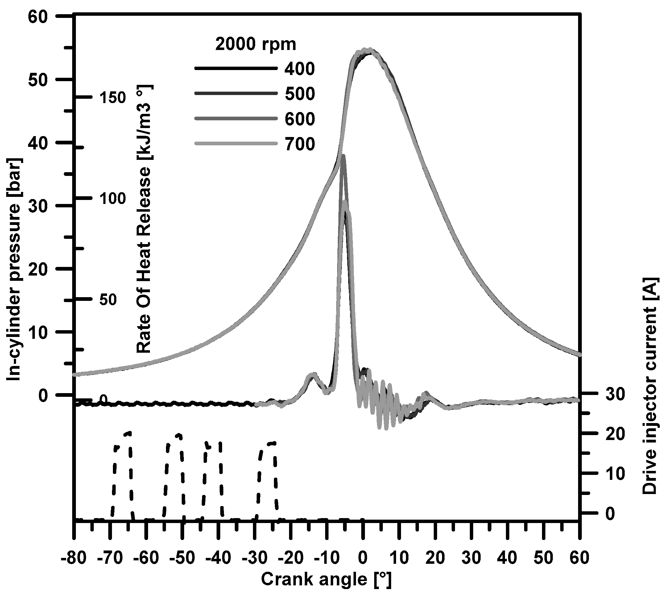
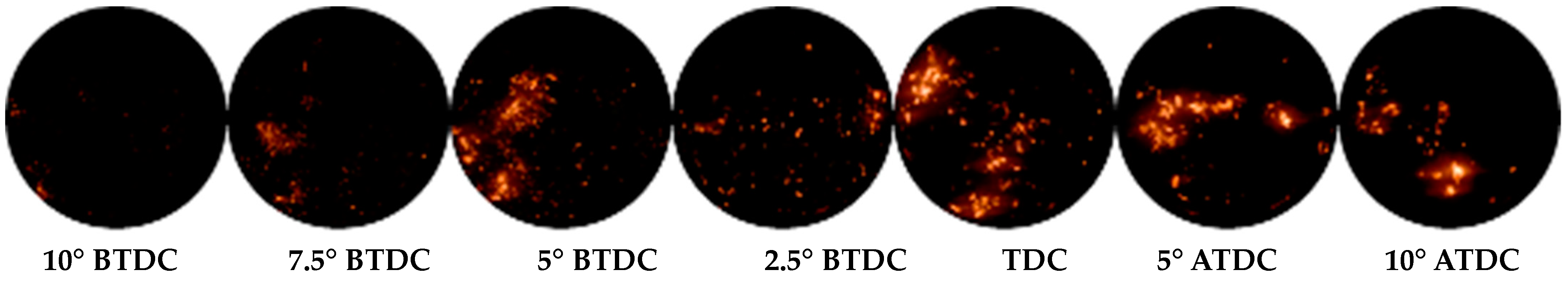
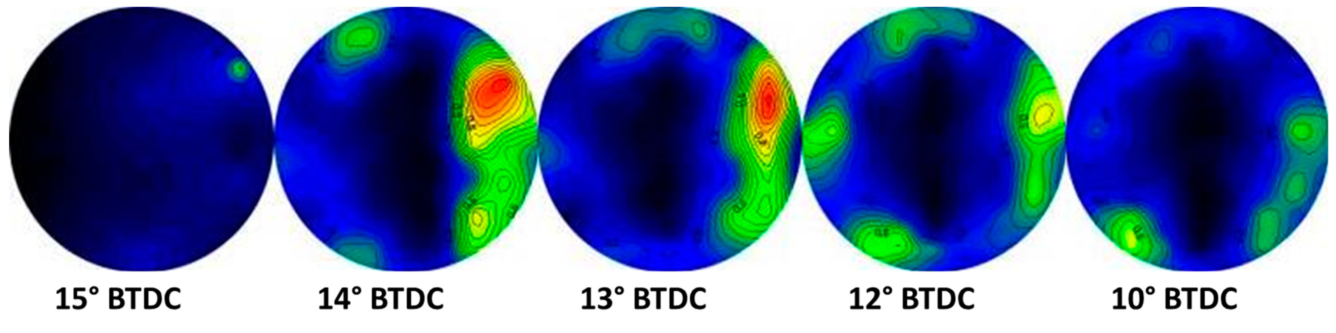
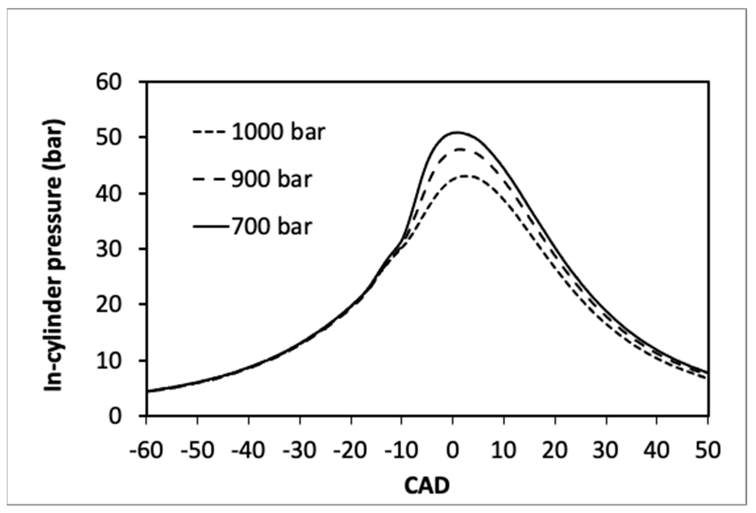
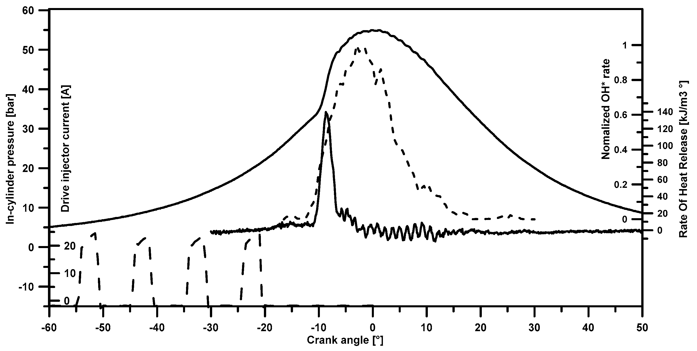
4.1. Experimental Results

In Figure 2, the experimental in-cylinder pressure and the rate of heat release curves at varying injection pressure are shown when the cycle includes four early injections and the engine speed is fixed at 2000 rpm. In this figure, the drive injector current is referred to the strategy with 400 bar injection pressure and, as reported in Table 2, shows clearly the four early injection events. The injection current signals of the other injection strategies at 2000 rpm and at higher injection pressure are with the same SOI and shorter duration are not reported in the figure to avoid difficulties in the reading of the graph. On the other hand, the rates of heat release curves show a premixed shape characteristic of HCCI combustion; in particular, two well-resolvable peaks can be recognized. They are not directly linked to the early injections and they prove the good mixing of the fuel with the air during the compression stroke. The injection delay with respect to the first injection is greater than 9.1 ms. Starting from the autoignition, the low temperature phase, and the following combustion evolution due to the development of high temperature regime can be recognized [18,32]. At 2000 rpm, varying injection pressure, no significant variation in combustion pressure, and ROHR developments are noted. At 1500 rpm and 1000 rpm (Table 2), the same combustion regimes of HCCI process are observed and well recognizable.

Visible images of combustion obtained through the piston crown window at 2000 rpm and at 700 bar of injection pressure are presented in Figure 3. This figure shows that for this engine operation, the HCCI process is reached. In addition, this figure shows small luminous spots randomly distributed at 10 CAD BTDC. As observed, these luminous spots are positioned in the boundary region. Over 10 CAD BTDC, the air motion moves these luminous spots over the entire cylinder volume during the compression stroke. In addition, from 10 CAD BTDC up to 10 CAD ATDC, the combustion behaves as premixed mode and the ignition does not take place in plainly homogeneous conditions.

By means of the UV imaging with “ad hoc” filter at 310 nm, the natural emission of the OH radical during the combustion evolution was detected. As an example, Figure 4 shows OH spatial distribution obtained at 1000 rpm and 700 bar of injection pressure. The radical OH distribution from 15 CAD BTDC down to 10 CAD BTDC seems to follow the combustion process of Figure 5. As observed in Figure 4, the OH radical concentration increases quickly around 14 CAD BTDC where the main ignition (the high temperature heat release region) occurs.

In all cases of Table 2, the experimental observations have confirmed that HCCI combustion process occurs in quasi-homogeneous lean charge on the entire combustion chamber with the presence of luminous spots, as observed on Figure 3. In addition, for all cases, the increase in OH radical during the cycle when the main ignition occurs has been observed. The experimental observations describing the evolution of OH radical during the cycle point out that this radical seems to be a good indicator to detect the start of high temperature heat release and phase the rate of heat release.

The experimental in-cylinder profiles with five early injections strategy at varying rail pressure when the engine speed is equal to 1000 rpm are reported in Figure 5. The inlet pressure is set equal to atmospheric pressure for this engine operation, whereas the inlet temperature was equal to 317 K. As observed on this figure, the highest in-cylinder pressure is achieved when the rail pressure is set equal to 700 bar and the lowest is obtained at 1000 bar of rail pressure. These slight pressure differences are due to fuel impingement observed experimentally when the injection pressure becomes higher than 700 bar (details are given in reference [21]). The impingement fuel mass does not take part in the combustion process and remains as unburned hydrocarbons. Figure 5 indicates, equally, that autoignition is not affected by the amount of impinged fuel mass and occurs for all strategies around 22 CAD BTDC for the first stage ignition (low temperature regime) and the combustion happens exclusively in a premixed mode.

It can be noted that at 2000 rpm, where the injection pressure is lower or equal to 700 bar, the fuel impingement phenomenon is not observed leading to the same in-cylinder pressure profiles as observed in Figure 2. The same trend has been observed [6] when the engine speed is fixed equal to 1500 rpm and the injection pressure is lower or equal to 700 bar.

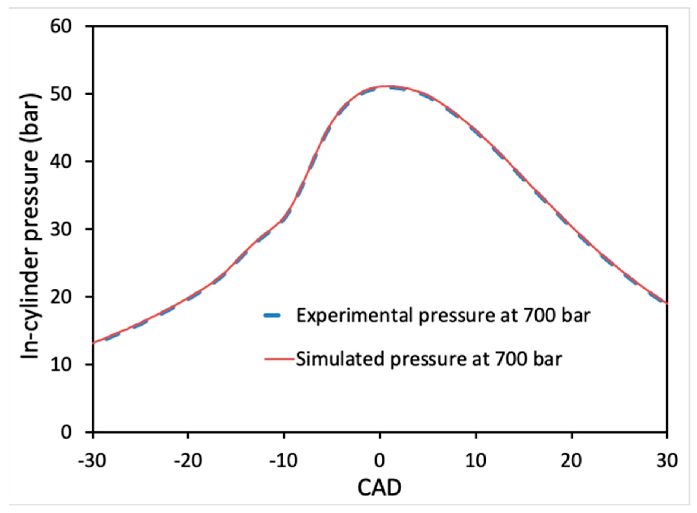
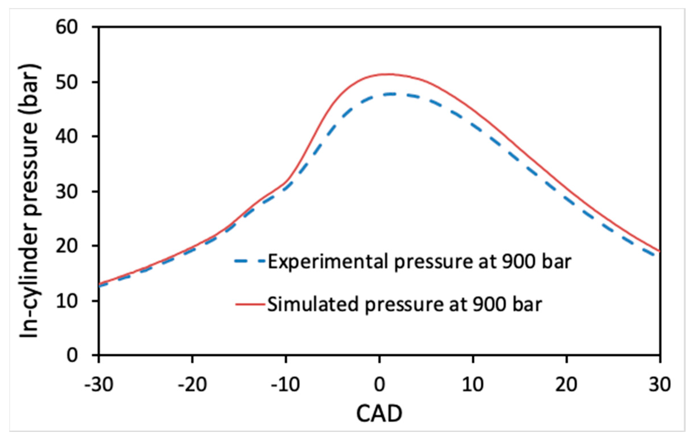
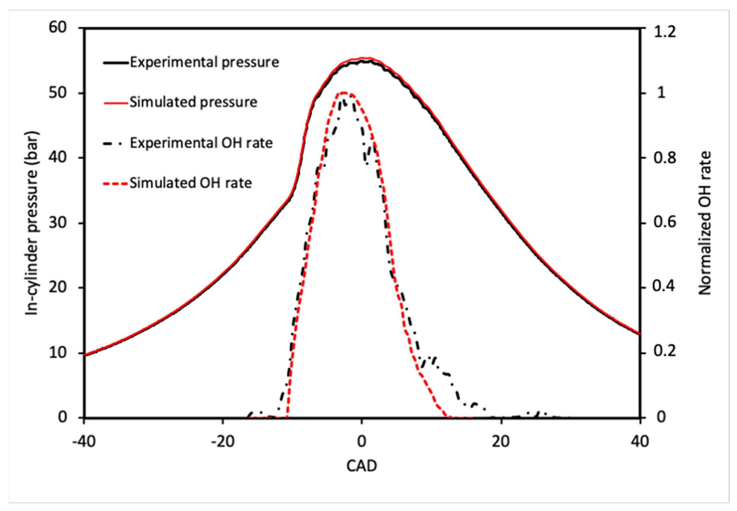
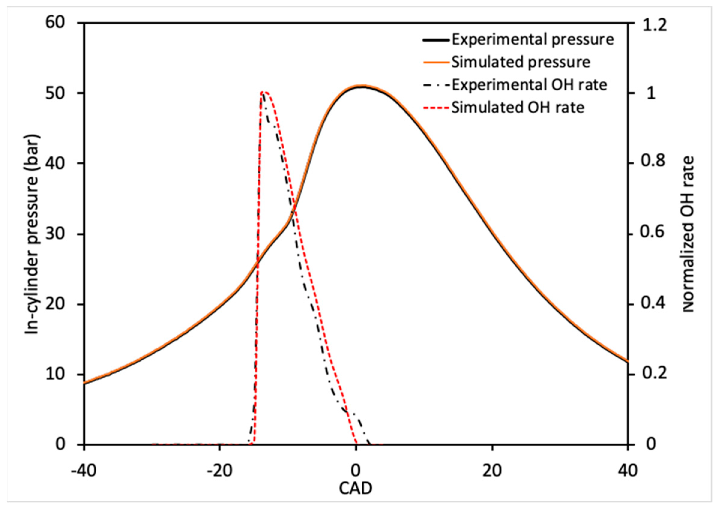
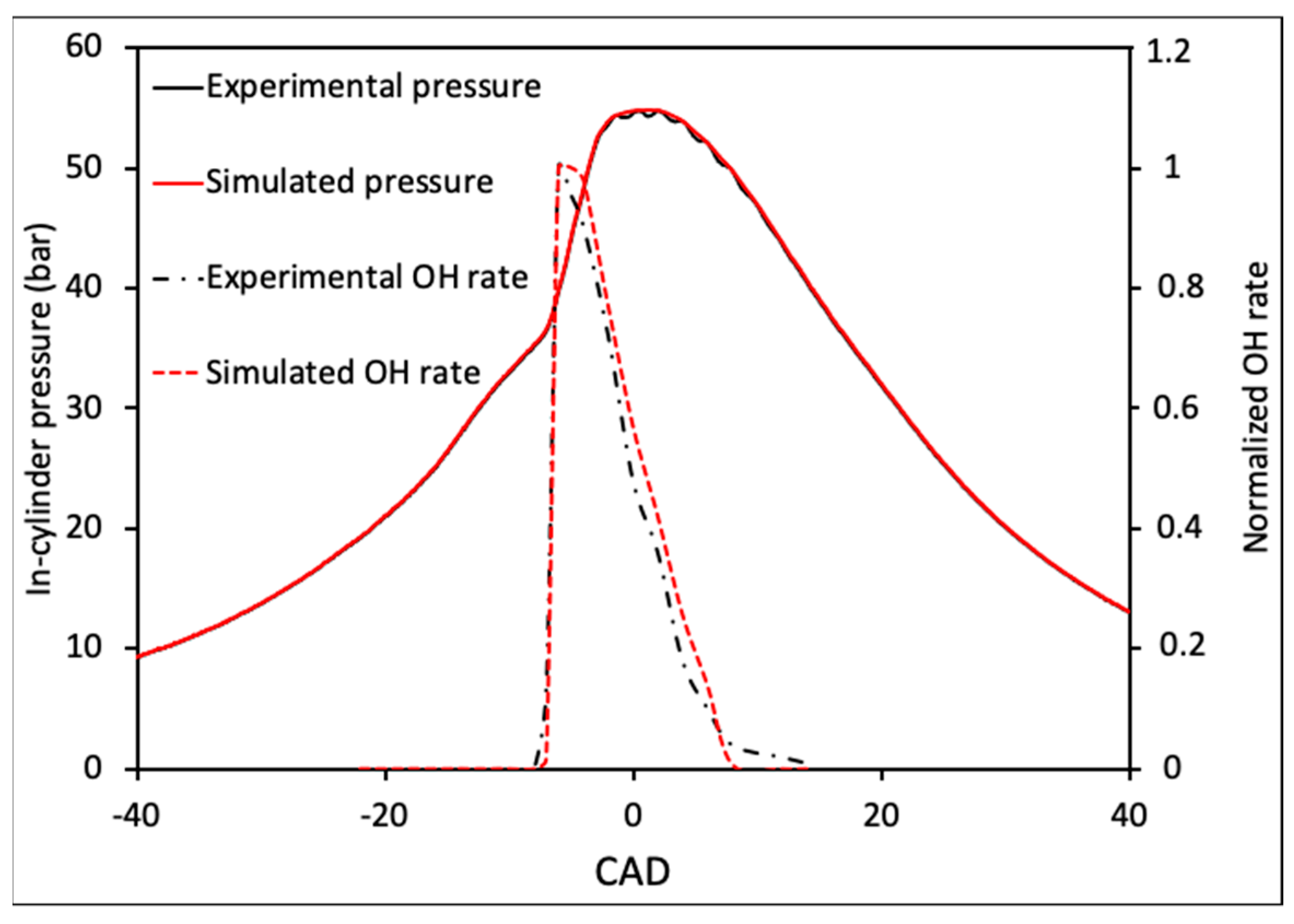
4.2. In-Cylinder Model Validation

In order to perform further validation of the in-cylinder model presented in Section 3, comparisons of simulations against experimental measurements have been performed. All numerical simulations were performed with initial conditions corresponding to the engine intake measured parameters. These mean intake conditions allow to calculate the random initial mass and initial temperature of each species and of each particle. All simulations used 200 particles and normal distribution [16]. The chemical reaction term has been simulated with the previous semi-reduced mechanism of n-heptane oxidation with 37 species and 61 elementary chemical reactions [18]. This chemical mechanism is able to simulate with more accuracy OH radical mass, compared to the precedent reduced mechanism of n-heptane oxidation [18] with 25 species and 26 elementary chemical reactions.

The comparison of measured and calculated in-cylinder pressures are shown in Figure 6, when the injection pressure is equal to 700 bar and engine speed fixed at 1000 rpm. Figure 7 reproduces the in-cylinder traces for the same engine speed and at 900 bar of injection pressure. As expected, at 900 bar the simulated in-cylinder pressure profile is higher compared to the measured trace (Figure 7). The pressure profile simulated at this injection pressure is similar to those obtained numerically and experimentally when the injection pressure is equal to 700 bar (Figure 6). This model behavior is due to the fact that the model did not include the description of the fuel impingement. Moreover, as observed in these figures, the same trends were obtained in terms of the first stage ignition delay and second stage ignition delay for both injection pressures, meaning that the amount of unburned fuel is very low. At 700 bar, Figure 6 shows that a good agreement for auto-ignition and peak of pressure is reached between the results predicted by the model and the measurement. In all cases, the mean relative error is lower than 2%.

In this study for OH species detection, the ICCD was used and coupled with narrow filters corresponding to 310 nm. Spectra and images were acquired in sets of 10 or 20, from 10 or 20 separate combustion cycles. The simulated OH rate evolution given by the reaction mechanism including 37 species and 61 elementary chemical reactions have been used to calculate the rate of OH. This rate represents the mass of OH radical divided by the maximum OH mass.

As an example, the measured OH rate profile is shown in Figure 8 when the engine speed is equal to 1500 rpm and the injection pressure set at 700 bar. This figure points out that the OH rate evolves during the high temperature regime and the increase in OH radical amount occurs at the same time than the main ignition. The qualitative comparison of measured and calculated OH rates during the main ignition for the same engine operation are shown in Figure 9. As observed in this figure the simulated OH rate profile has the same shape as the measured OH trace and the main ignition occurs at the same time. Moreover, the simulated OH rate evolves also during the high temperature regime as observed experimentally. This OH evolution shape has been observed experimentally by Collin et al. [33], where the OH radical has been measured by Laser Induced Fluorescence (LIF) at the wavelength of 283 nm. However, the authors have found that the OH-LIF intensity was lagging the main ignition time by about 8 CAD, which is not the case in the present study. This difference may be explained by the early small injections strategy reported in Table 2 and adopted in this study. Figure 9 also reproduces the comparison of measured and of simulated in-cylinder pressure profiles. As observed on this figure, the ignition delay time and maximum peak pressure are well reproduced by the model for this engine operating point.

Comparison of OH rate profiles at 1000 rpm is presented in Figure 10 (see also Figure 4 above). This latter shows the same behavior as observed in Figure 9, in term of ignition delay time. However, this figure points-out that the evolution of OH rates is stiff during the main ignition, meaning that for this engine operating point the mixture is homogeneous in the combustion chamber [26,34]. This homogeneity is mostly due to the early injection in the cycle (pilot at −70 CAD BTDC). The same stiffness shown in Figure 11 is obtained when the engine speed is fixed at 2000 rpm with the same timing of pilot injection (see Table 2) at 700 bar injection pressure. For these two cases, the calculated confidence coefficient is equal to 8.4% at 1500 rpm and equal to 7.9% at 2000 rpm, meaning that the mixture is almost homogeneous. When the engine speed is fixed at 1500 rpm and the pilot injection is retarded at −50 CAD BTDC, the OH radical rates increase is less pronounced, as shown in Figure 9. In this case the confidence coefficient is equal 14.2%, leading to higher heterogeneity of the mixture, in comparison with the results of Figure 10. Equation (14) points out that when the engine speed decreases from 2000 rpm down to 1000 rpm, the initial mean kinetic energy decreases inducing an increase in the confidence coefficient. These trends are in agreement with the experimental observations concerning in-cylinder pressure and OH rate behaviors at varying engine speed. Consequently, the correlation retained (Equation (17)) in this study to model the confidence coefficient (initial heterogeneities of the mixture) describes with a good agreement the initial heterogeneities. In addition, the timing of injection in the cycle has also an important effect on the quality of the mixture. For this reason, the confidence coefficient is higher at 1500 rpm, in comparison with the values obtained at 1000 rpm and 2000 rpm.

Thereby, a direct comparison of numerical results from the stochastic reactor model including a turbulence model on the combustion process, shows that the calculations are good in their general description of OH radical profiles, which are in resemblance of the measurements at varying engine speed and injection strategy.

5. Conclusions

In the present study, imaging and chemiluminescence measurements from ultraviolet (UV) to visible were performed by means of the optical set up, in order to investigate performances and indicated rate about the in-cylinder LTC combustion progress. Two injection strategies based on four and five early injections in the cycle were used at different engine speeds. In addition, the natural emission of the OH radical during the combustion evolution was detected.

In parallel, LTC combustion model was used based on the particles approximation of the PDF transport equation. In this model, the micro-mixing was treated through an IEM model, which is an appropriate approach to describe the interaction of turbulence with chemistry and to take into account the heterogeneities of the mixture in the combustion chamber via a stochastic method. This previous IEM model was extended in order to include a turbulent time scale model linked to the turbulent kinetic energy and its dissipation. The confidence coefficient retained in this study and reflecting the initial inhomogeneities amplitude of temperature and of species mass was expressed as a function of the turbulent Reynolds number. This approach allows to develop complete and autonomous models to describe LTC process taking into account the effects of flow and turbulence, which are an important challenge.

Visible images of combustion at varying engine operating conditions have confirmed that the premixed combustion mode during the cycle is reached and that the ignition did not occur in plainly homogeneous mixtures. In all cases investigated in this study, the experimental observations have indicated that LTC process takes place in quasi-homogeneous lean mixture in the entire combustion chamber characterized by luminous spots. Autoignition was treated by UV-visible chemiluminescence and the OH radical was detected homogeneously distributed.

The in-cylinder pressures predicted by the model were validated against the experimental results. This step points out that they present the same behavior in terms of homogenous combustion, and of ignition delay times. At varying injection pressure, the experimental observations point out that when the injection pressure exceeds 700 bar the fuel impingement on the wall becomes higher, in comparison with the cases when the injection pressure is lower than 900 bar. In the case when the fuel impingement exceeds a certain level, the model did not include this phenomenon leading to a difference between simulated and measured in-cylinder pressure trace. However, for all engine operations when the injection pressure in lower or equal to 700 bar, an excellent agreement is obtained between the results predicted by the model and the measurements for the in-cylinder profiles, the mean relative error is lower than 2%.

The qualitative comparison of measured and calculated OH rates during the main ignition has been investigated. This step has shown that the simulated OH profiles have the same shape as the measured OH traces and the main ignition occurs at the same time. The experimental results at varying engine speed have shown that when the engine speed decreases the homogeneity of the mixture decreases. These observations are in agreement with the results of the confidence coefficient included in the model. Indeed, the calculated confidence coefficient values decrease when the engine speed increases, meaning that the homogeneity of the mixture becomes higher. In addition, at varying injection strategies, the experimental observations and the simulated confidence coefficient indicates that early injection in the cycle is in favor for homogeneous mixture. In addition, this study confirms that the OH radical is a suitable tool to identify the start of high heat release rate and phase the rate of heat release.

The combustion processes in HCCI and/or LTC mode are primarily controlled by chemical kinetics; this is why several studies have been targeted to different chemical kinetic reaction mechanisms for different fuel development. However, there is still attention to be put on the effects of flow or of turbulence on combustion processes. The experimental observations of this study have shown that there is still inhomogeneous charge in local area of the combustion chamber. Consequently, the turbulence mixing and the interaction of turbulence with chemistry have a larger effect on LTC and or HCCI conditions. This study was performed to contribute to this challenging objective. In addition, the global developed model can be used regardless of fuel type (i.e., kinetic reaction mechanism).

References

1. Krishnamoorthi, M.; Malayalamurthi, R.; Zhixia, H.; Sabariswaran, K. A review on low temperature combustion engines: Performance, combustion and emission characteristics. Renew. Sustain. Energy Rev. 2019, 116, 109404. [Google Scholar] [CrossRef]
2. Saxena, S.; Bedoya, I.D. Fundamental phenomena effecting low temperature combustion and HCCI engines, high load limits and strategies for extending these limits. Prog. Energy Combust. Sci. 2013, 39, 457–488. [Google Scholar] [CrossRef]
3. Yao, M.; Zheng, Z.; Liu, H. Progress and recent trends in homogeneous charge compression ignition (HCCI) engines. Prog. Energy Combust. Sci. 2009, 35, 398–437. [Google Scholar] [CrossRef]
4. Hultqvist, A.; Christensen, M.; Johansson, B.; Richter, M.; Nygren, J.; Hult, J.; Aldén, M. The HCCI combustion process in a single cycle-high-speed fuel tracer LIF and chemiluminescence imaging. SAE Trans. 2002, 111, 913–927. [Google Scholar]
5. Richter, M.; Engstrom, J.; Franke, A.; Aldén, M.; Hultqvist, A.; Johansson, B. The Influence of Charge Inhomogeneity on the HCCI Combustion Process; SAE Technical Paper 2000-01-2868; SAE International: Warrendale, PA, USA, 2000. [Google Scholar]
6. Mancaruso, E.; Vaglieco, B.M. Optical investigation of the combustion behaviour inside the engine operating in HCCI mode and using alternative diesel fuel. Exp. Therm. Fluid Sci. 2010, 34, 346–351. [Google Scholar] [CrossRef]
7. Christensen, M.; Johansson, B. The Effect of In-Cylinder Flow and Turbulence on HCCI Operation; SAE Technical Paper 2002-01-2864; SAE International: Warrendale, PA, USA, 2002. [Google Scholar]
8. D’Amato, M.; Viggiano, A.; Magi, V. On turbulence-chemistry interaction of an HCCI combustion engine. Energies 2020, 13, 5876. [Google Scholar] [CrossRef]
9. Kong, S.C.; Reitz, R.D.; Christensen, M.; Johansson, B. Modeling the effects of geometry generated turbulence on HCCI engine combustion. SAE Trans. 2003, 112, 1511–1521. [Google Scholar]
10. Pope, S.B. PDF Methods for Turbulent Reactive Flows. Prog. Energy Combust. Sci. 1985, 11, 119–192. [Google Scholar] [CrossRef]
11. Dopazo, C.; O’Brien, E.E. An Approach to the Autoignition of a Turbulent Mixture. Acta Astronaut. 1974, 1, 1239–1266. [Google Scholar] [CrossRef]
12. Curl, R.L. Dispersed phase mixing: I. Theory and effects in simple reactors. AIChE J. 1963, 9, 175–181. [Google Scholar] [CrossRef] [Green Version]
13. Hsu, A.T.; Tsai, Y.L.P.; Raju, M.S. Probability Density Function Approach for Compressible Turbulent Reacting Flows. AIAA J. 1994, 32, 7. [Google Scholar] [CrossRef]
14. Subramaniam, S.; Pope, S.B. A Mixing Model for Turbulent Reactive Flows based on Euclidean Minimum Spanning Trees. Combust. Flame 1998, 115, 487–514. [Google Scholar] [CrossRef]
15. Yang, B.; Pope, S.B. An Investigation of the Accuracy of Manifold Methods and Splitting Schemes in the Computational Implementation of Combustion Chemistry. Combust. Flame 1998, 112, 16–32. [Google Scholar] [CrossRef]
16. Pommier, P.L.; Maroteaux, F.; Sorine, M.; Ravet, F. Particle Approximation Applied to Diesel Combustion: Effects of Initial Distribution and Particles Number; SAE Technical Paper 2007-24-0033; SAE International: Warrendale, PA, USA, 2007. [Google Scholar]
17. Pommier, P.L.; Maroteaux, F.; Sorine, M. A PDF method for HCCI combustion modeling CPU time optimization through a restricted initial distribution. Mech. Ind. 2012, 13, 219–228. [Google Scholar] [CrossRef]
18. Maroteaux, F.; Noel, L. Development of a reduced n-heptane oxidation mechanism for HCCI combustion modeling. Combust. Flame 2006, 146, 256–267. [Google Scholar] [CrossRef]
19. Maroteaux, F.; Pommier, P.L. A turbulent time scale based k-epsilon model for probability density function modeling of turbulence/chemistry interactions: Application to HCCI combustion. Int. J. Heat Fluid Flow 2013, 42, 105–114. [Google Scholar] [CrossRef]
20. Maroteaux, F.; Mancaruso, E.; Vaglieco, B.M. A Mixing Timescale Model for PDF Simulations of LTC Combustion Process in Internal Combustion Engines; SAE Technical Paper 2019-24-0113; SAE International: Warrendale, PA, USA, 2019. [Google Scholar] [CrossRef]
21. Heywood, J.B. Internal Combustion Engine Fundamentals; Mc Graw-Hill: New York, NY, USA, 1988. [Google Scholar]
22. Denbratt, I.; Helmantel, A. HCCI Operation of a Passenger Car Common Rail DI Diesel Engine with Early Injection of Conventional Diesel Fuel; SAE Technical Paper 2004-01-0935; SAE International: Warrendale, PA, USA, 2004. [Google Scholar]
23. Mancaruso, E.; Merola, S.S.; Vaglieco, B.M. Extinction and Chemiluminescence Measurements in CR DI Diesel Engine Operating in HCCI Mode; SAE Technical Paper 2007-01-0192; SAE International: Warrendale, PA, USA, 2007. [Google Scholar]
24. Villermaux, J.; Devillon, J.C. Représentation de la coalescence et de la redispersion des domaines de ségrégation dans un fluide par un modèle d’interaction phénoménologique. In Proceedings of the 2nd International Symposium on Chemical Reaction Engineering, Amsterdam, The Netherlands, 2–4 May 1972; Elsevier: New York, NY, USA, 1972. [Google Scholar]
25. Kraft, M.; Wolfgang, W. An Efficient Stochastic Chemistry Approximation for the PDF Transport Equation; WIAS-Publications: Berlin, Germany, 2001; ISSN 0946-8633. [Google Scholar]
26. Kraft, M.; Maigaard, P.; Mauss, F.; Christensen, M.; Johansson, B. Investigation of combustion emissions in a homogeneous charge compression injection engine: Measurements and a new computational model. Proc. Combust. Inst. 2000, 28, 1195–1201. [Google Scholar] [CrossRef]
27. Mitarai, S.; Riley, J.J.; Kosàly, G. Testing of mixing models for Monte Carlo probability density function simulations. Phys. Fluids 2005, 17, 047101. [Google Scholar] [CrossRef]
28. Assanis, D.N.; Heywood, J.B. Development and use of a computer simulation of the turbocompounded Diesel system for engine performance and component heat transfer studies. SAE Trans. 1986, 95, 451–476. [Google Scholar]
29. Pope, S.B. Turbulent Flows; Cambridge University Press: Cambridge, UK, 2000. [Google Scholar]
30. Fox, R.O. Computational Models for Turbulent Reactive Flows; Cambridge University Press: Cambridge, UK, 2003. [Google Scholar]
31. Fiveland, S.B.; Assanis, D.N. A four stroke homogeneous charge compression ignition engine simulation for combustion and performance studies. SAE Trans. 2000, 109, 452–468. [Google Scholar]
32. Emery, P.; Maroteaux, F.; Sorine, M. Modeling of combustion in GDI engines for the optimization of engine management system through reduction of 3D models to (n*1D) models. J. Fluids Eng. 2003, 125, 520–532. [Google Scholar] [CrossRef]
33. Collin, R.; Nygren, J.; Richter, M.; Aldén, M.; Hildingsson, L.; Johansson, B. Simultaneous OH and formaldehyde-LIF measurements in an HCCI engine. SAE Trans. 2003, 112, 2479–2486. [Google Scholar]
34. Assanis, D.N.; Najt, P.M.; Dec, J.E.; Eng, J.A.; Asmus, T.N.; Zhao, F. Homogeneous Charge Compression Ignition (HCCI) Engines, Key Research and Development Issues; SAE International: Warrendale, PA, USA, 2003. [Google Scholar]
Figure 1. (a) Optical engine and experimental apparatus for spectroscopic and imaging measurements. (b) Engine experimental setup.
Energies 16 03459 g001
Figure 2. Histories of in-cylinder pressures, rates of heat release, and drive injector current at 2000 rpm and varying injection pressure, with four injections strategy (intake pressure fixed at 2.4 bar).
Energies 16 03459 g002
Figure 3. Visible images at 2000 rpm and injection pressure fixed at 700 bar.
Energies 16 03459 g003
Figure 4. OH spatial distribution during auto-ignition and combustion phase at 1000 rpm at 700 bar.
Energies 16 03459 g004
Figure 5. Experimental in-cylinder traces versus CAD at 1000 rpm and varying injection pressure.
Energies 16 03459 g005
Figure 6. Comparison of the calculated in-cylinder pressure versus CAD with measured data at 1000 rpm and 700 bar.
Energies 16 03459 g006
Figure 7. Comparison of the calculated in-cylinder pressure versus CAD with measured data at 1000 rpm and 900 bar.
Energies 16 03459 g007
Figure 8. Experimental OH rate evolution when the injection pressure is equal to 700 bar and engine speed fixed at 1500 rpm, (intake pressure fixed at 1.7 bar).
Energies 16 03459 g008
Figure 9. Experimental and numerical OH rates and in-cylinder pressure profiles comparison when the injection pressure is equal to 700 bar and engine speed fixed at 1500 rpm.
Energies 16 03459 g009
Figure 10. Experimental and numerical of OH radical rates comparison when the injection pressure is equal to 700 bar and engine speed fixed at 1000 rpm.
Energies 16 03459 g010
Figure 11. Experimental and numerical of OH radical rates comparison when the injection pressure is equal to 700 bar and engine speed fixed at 2000 rpm.
Energies 16 03459 g011