
Conjugate Heat Transfer Modeling of a Cold Plate Design for Hybrid-Cooled Data Centers

 , ,
, , 
Abstract
:1. Introduction
2. Methods
2.1. Governing Equations
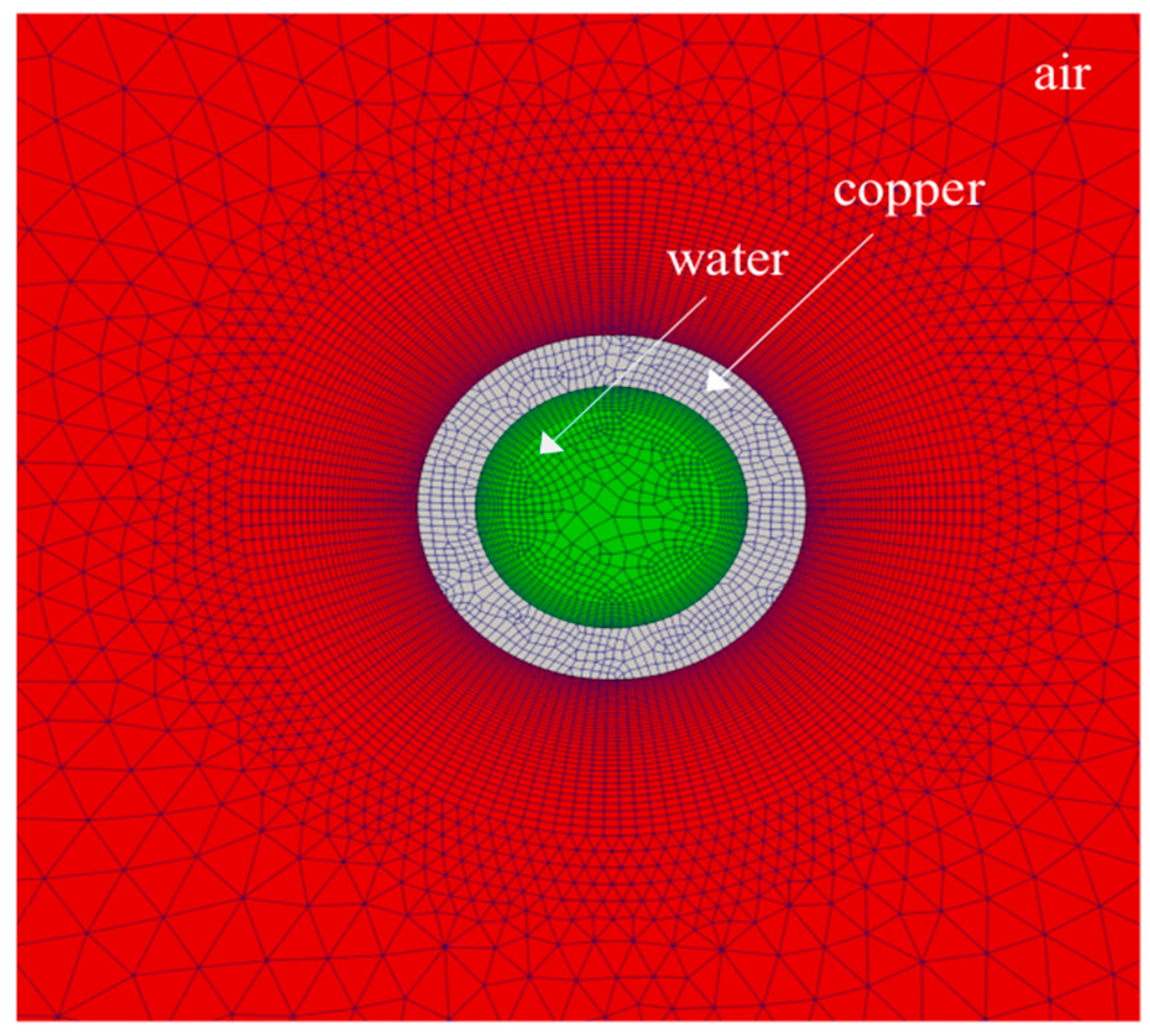
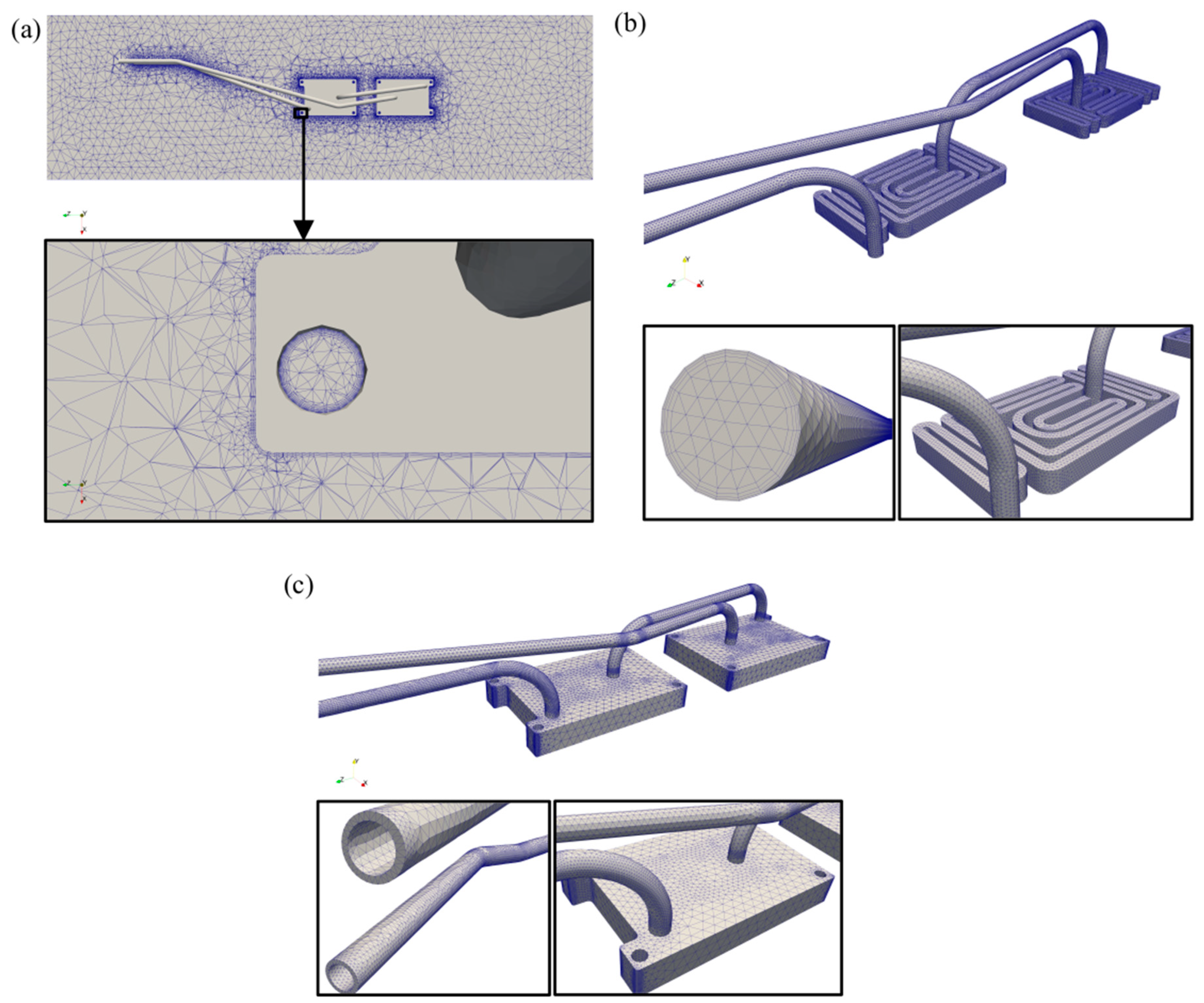
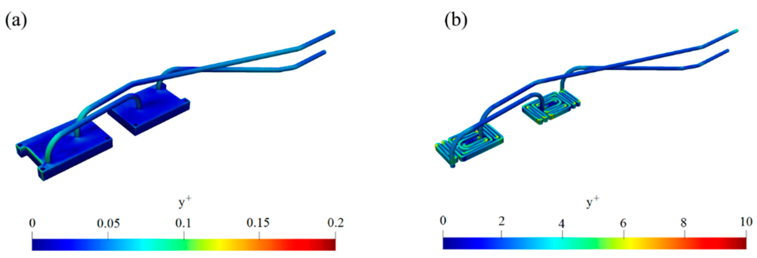
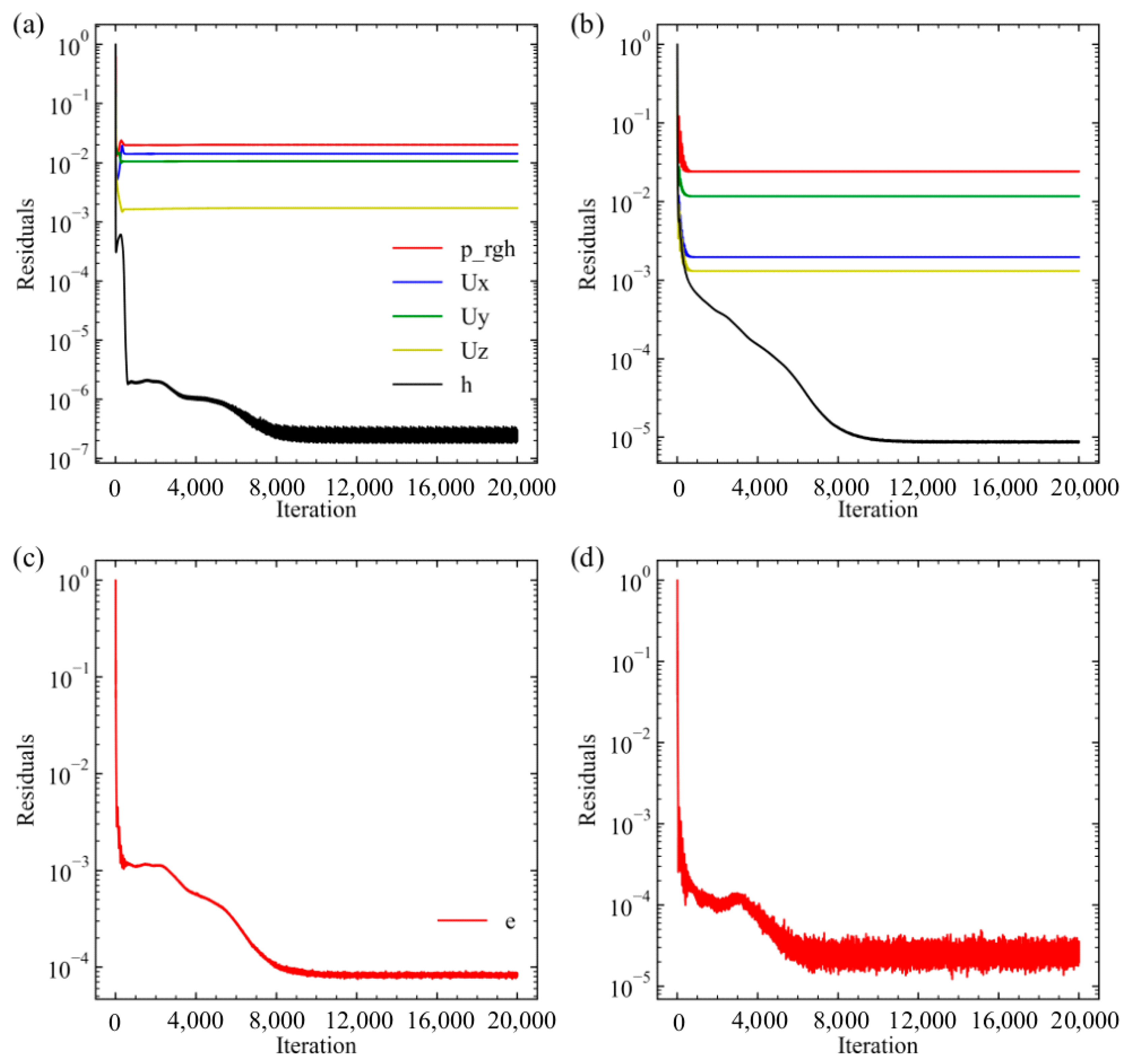
2.2. Numerical Model
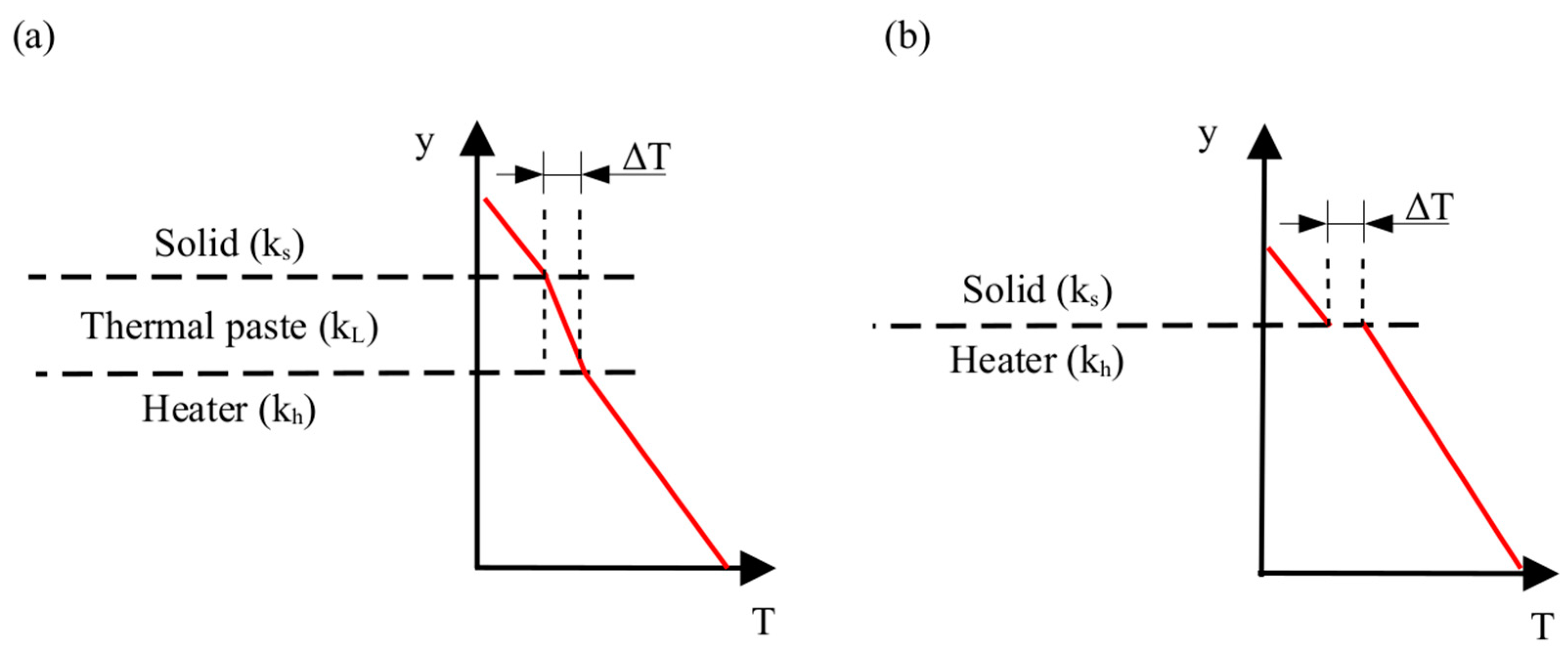
2.3. Modeling Thermal Paste
3. Results
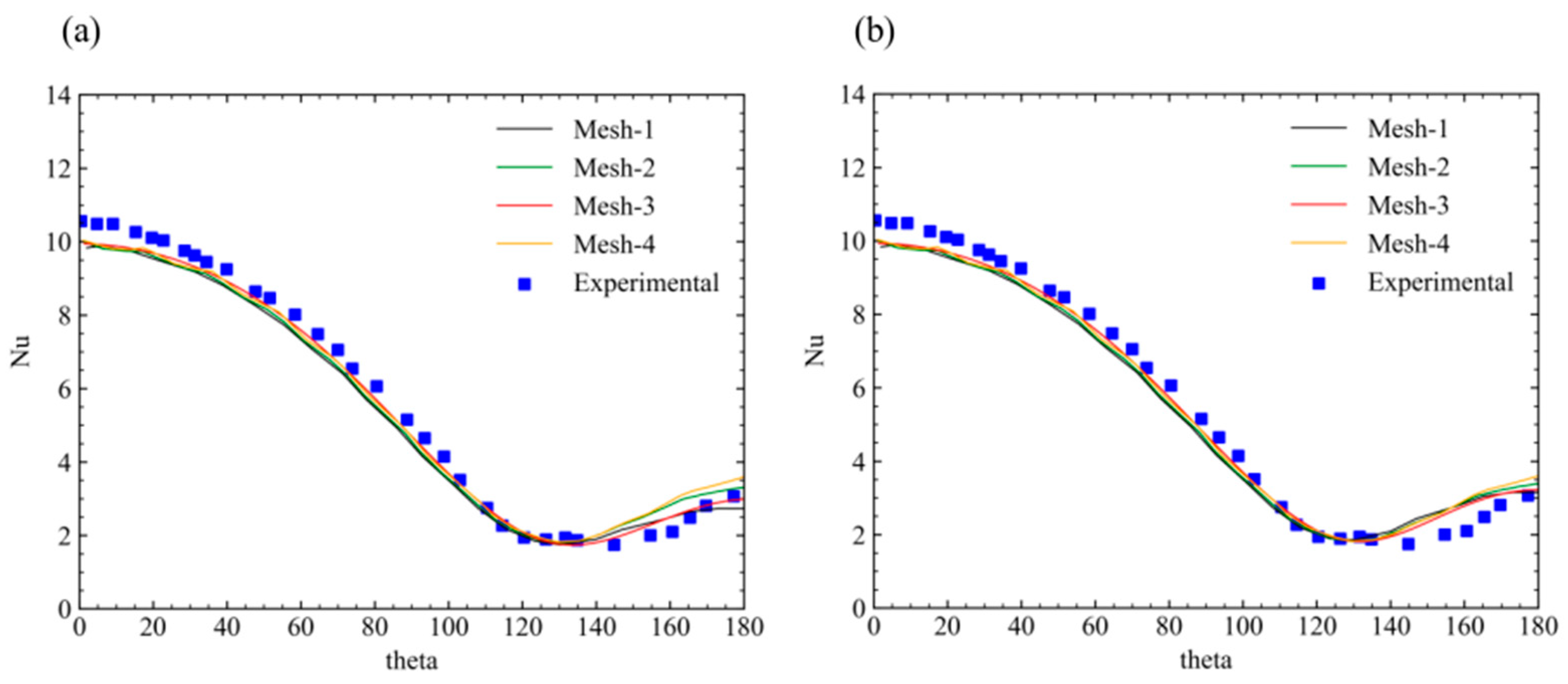
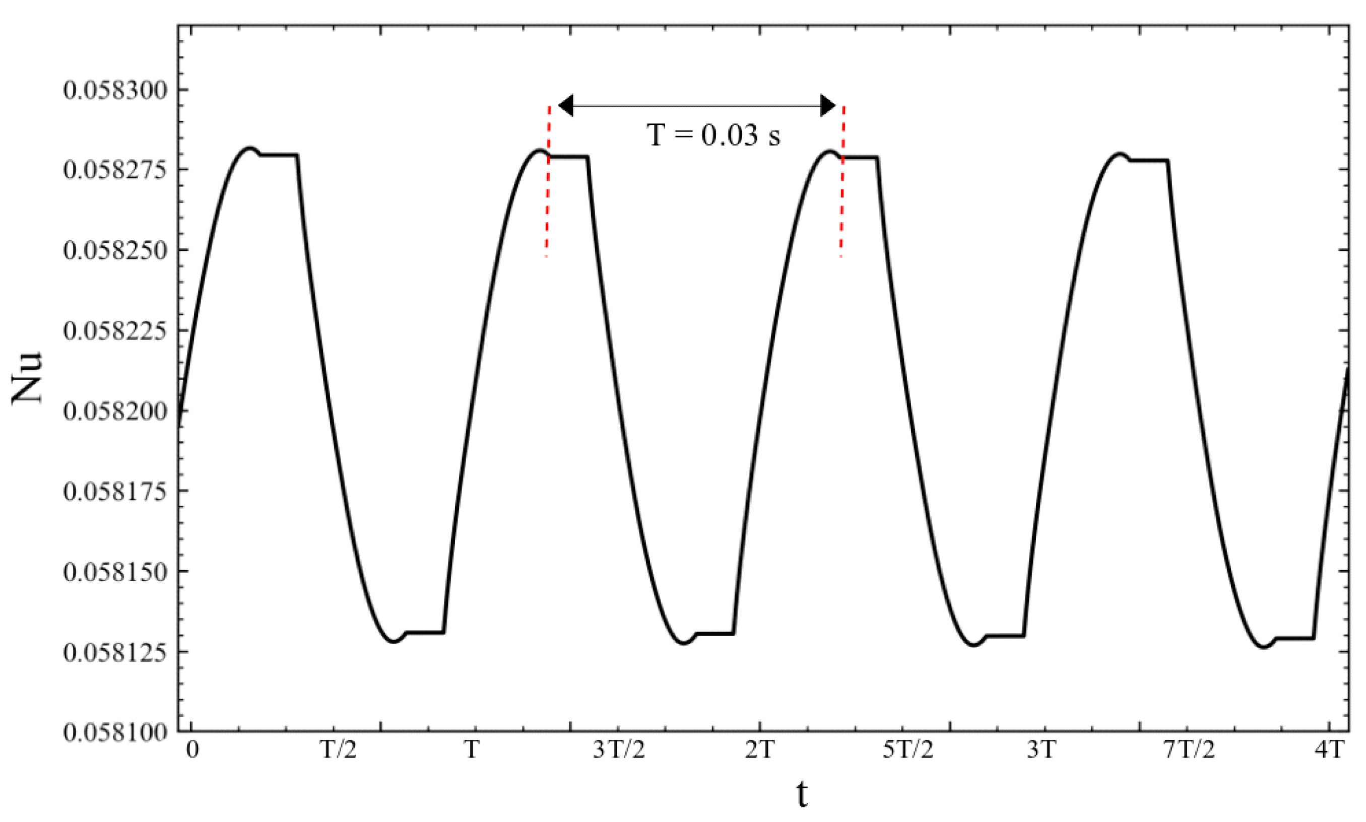
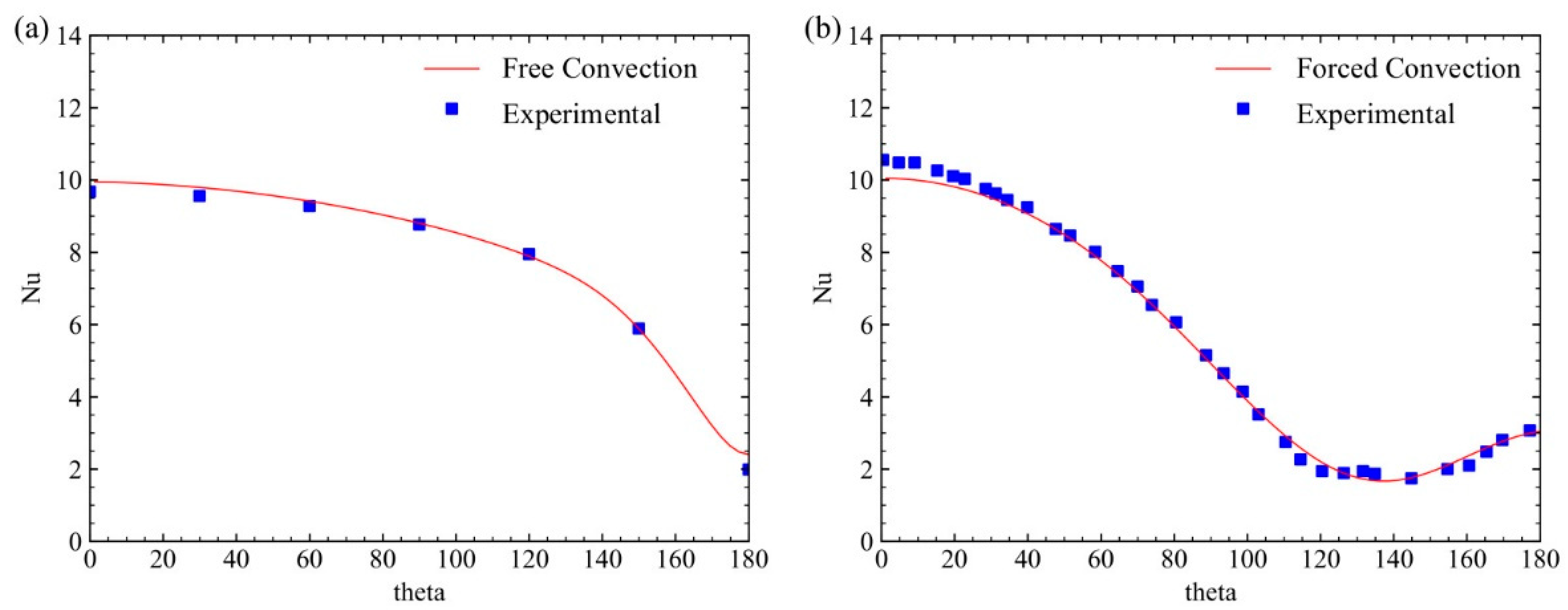
3.1. Validation of the CHT Model
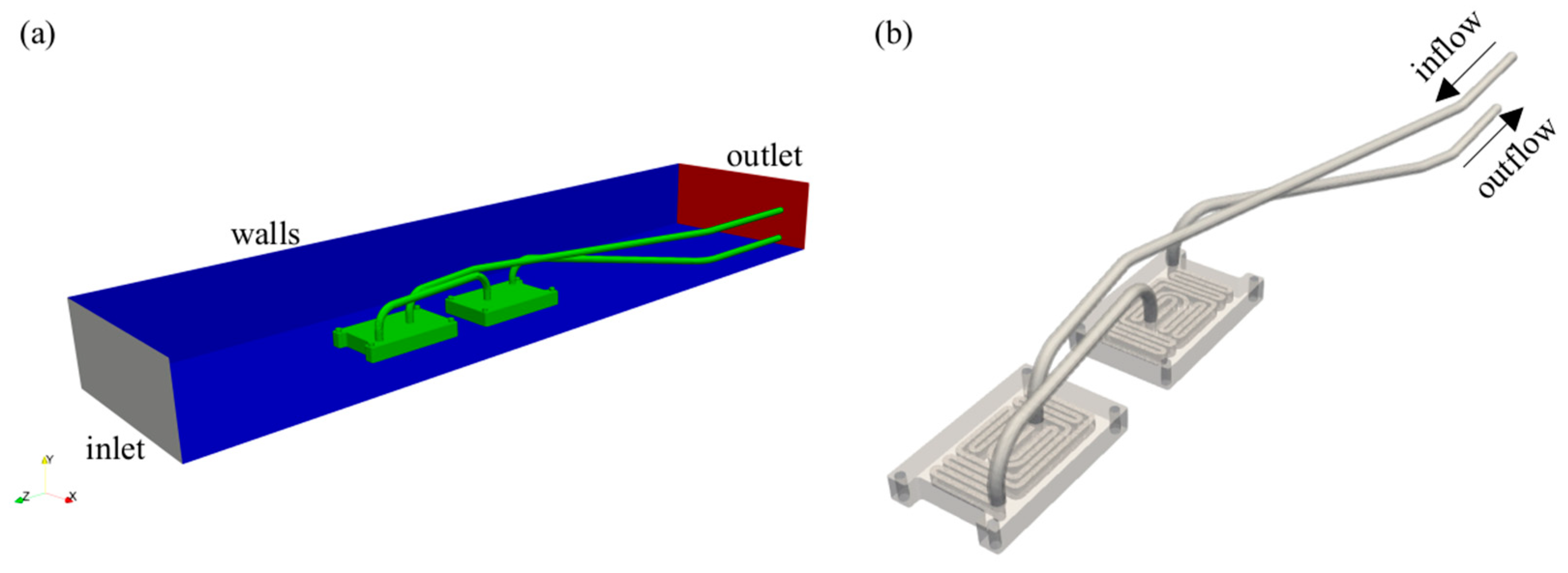
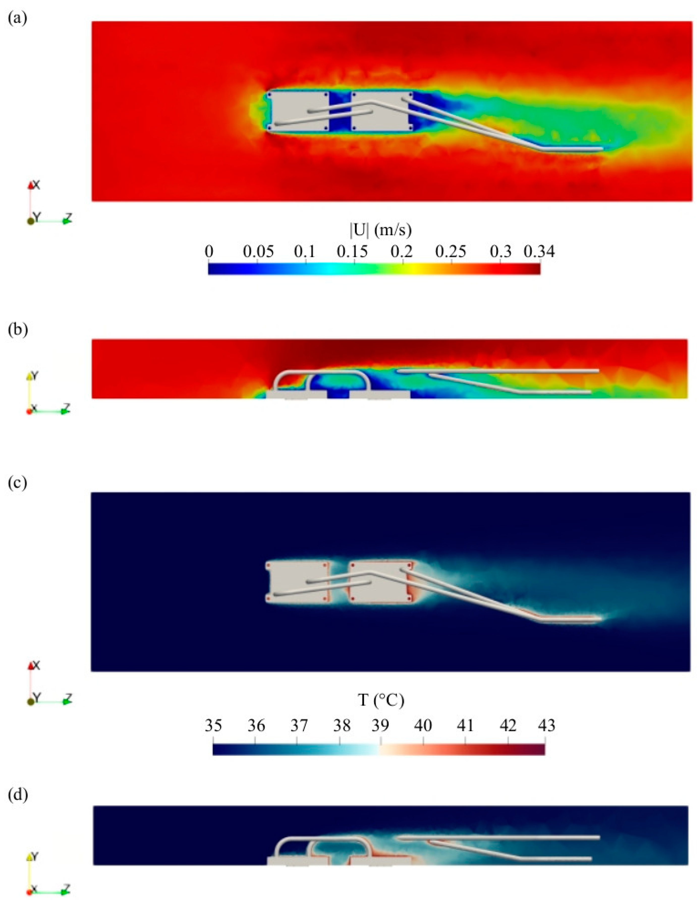
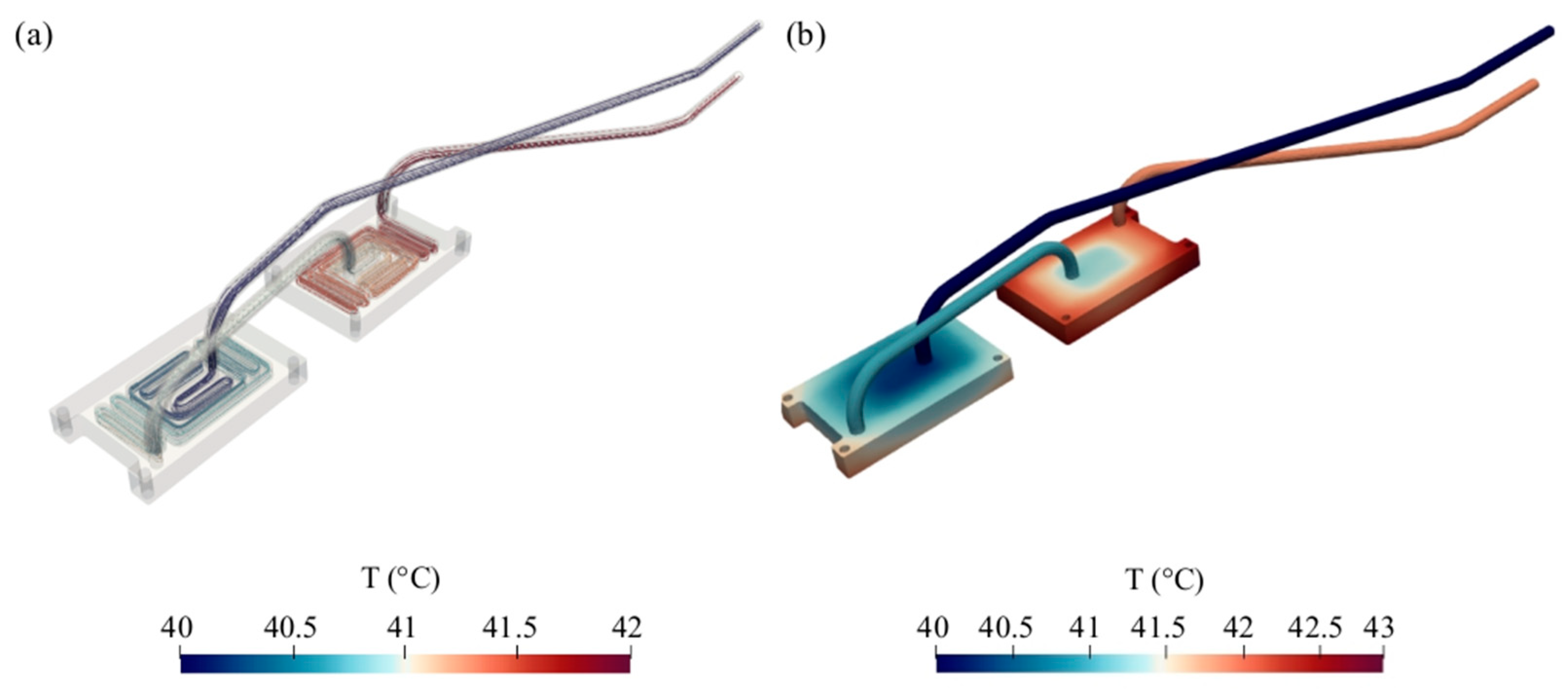
3.2. Thermal Simulation of the Cold Plate
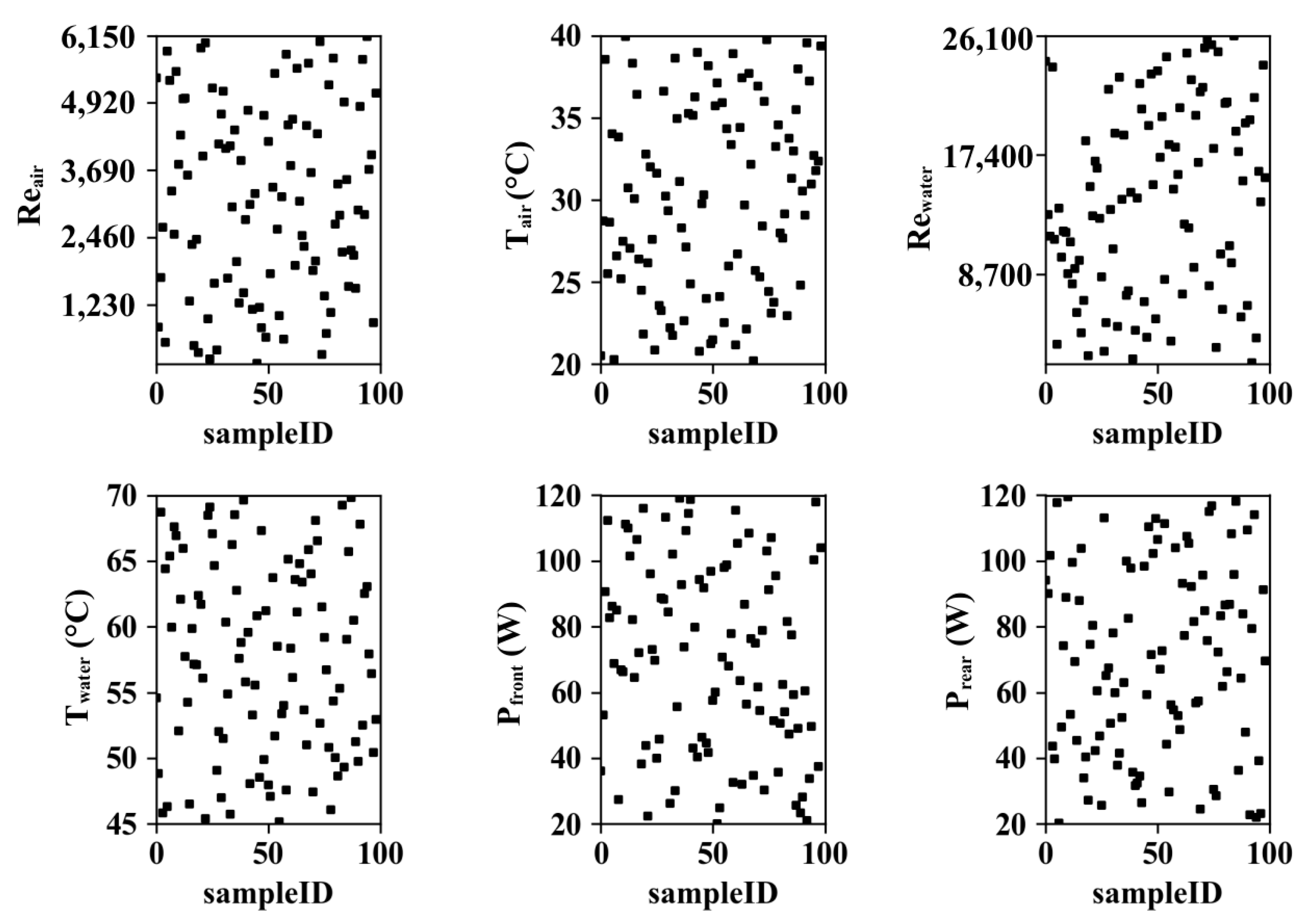
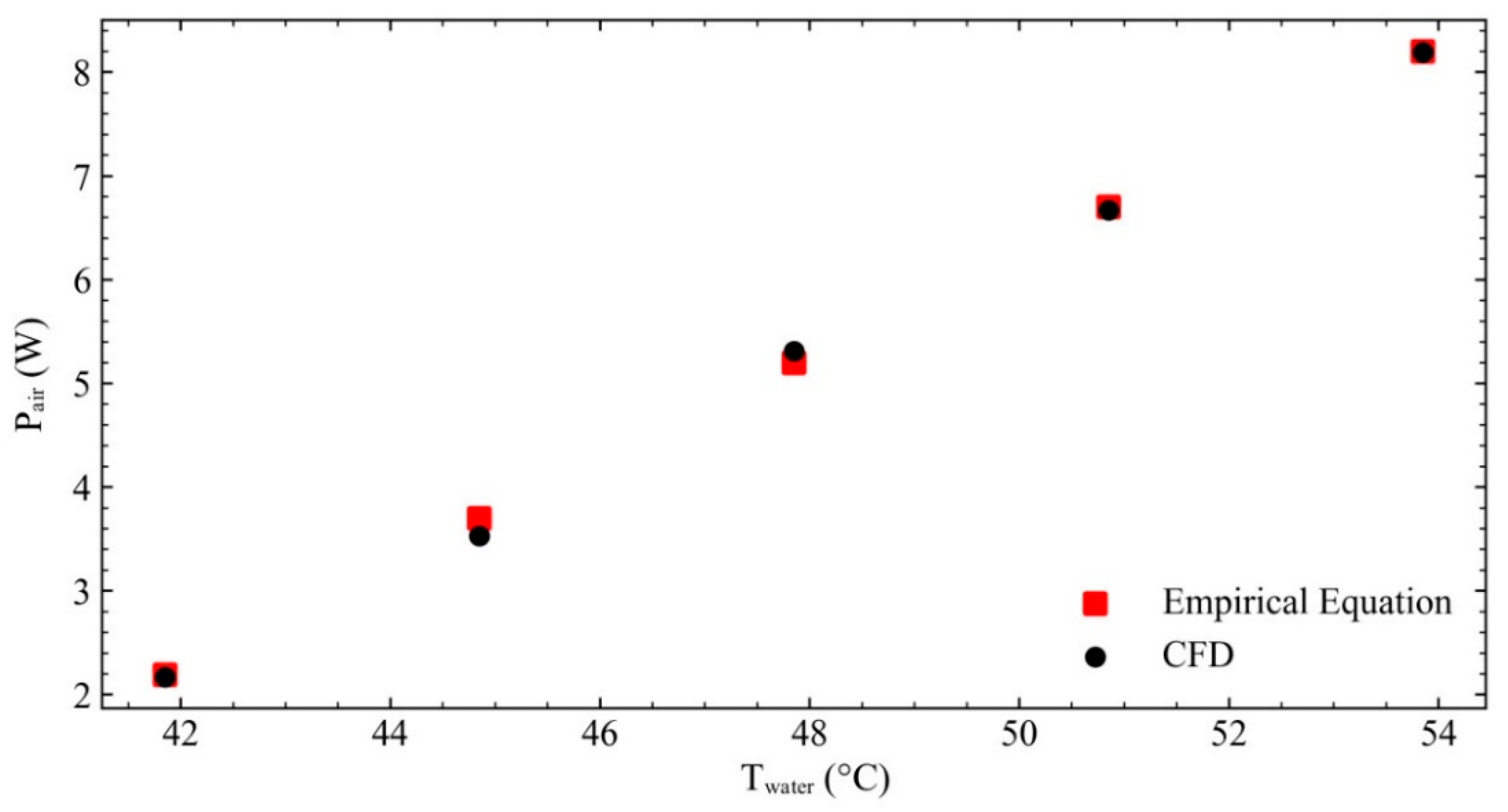
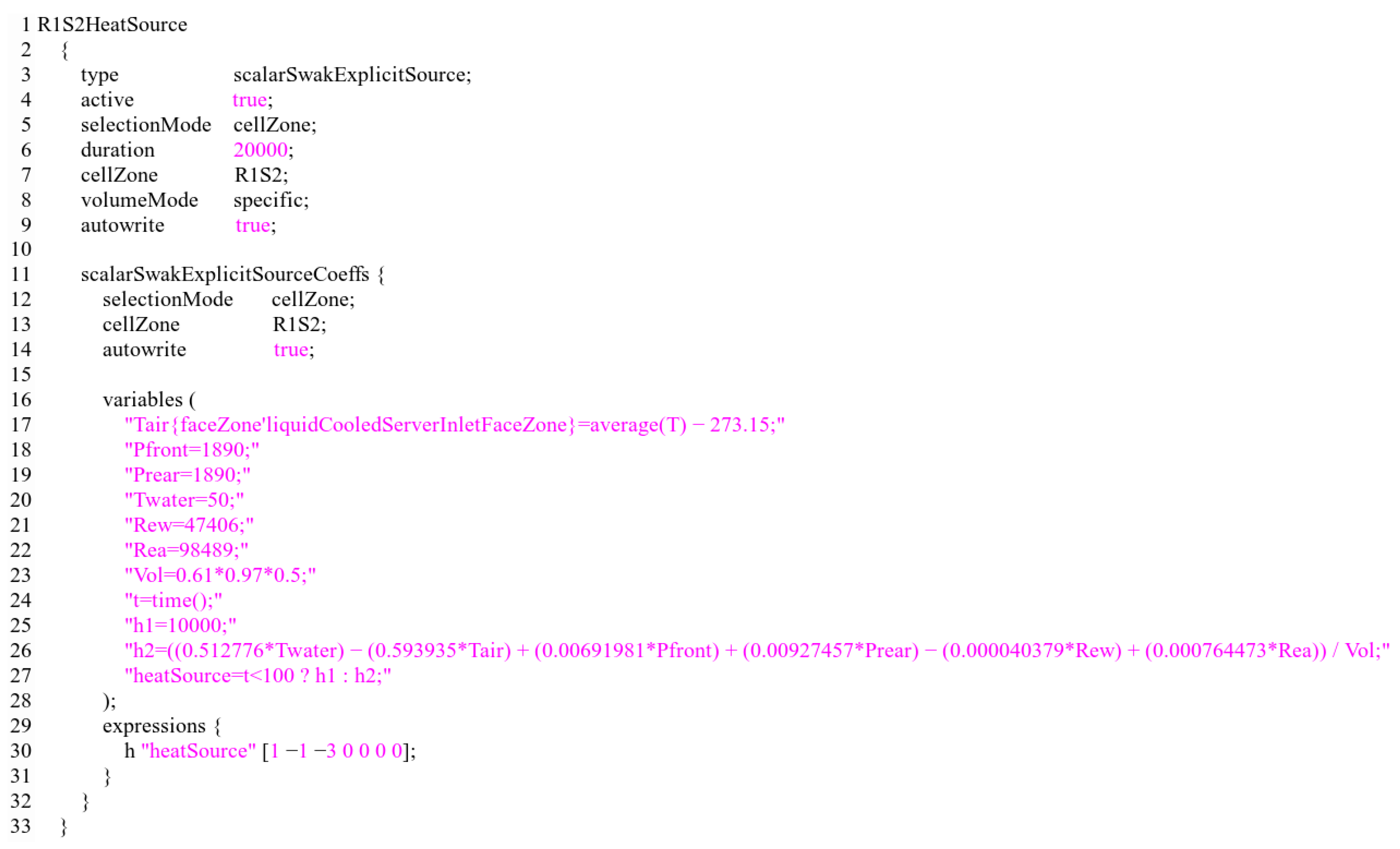
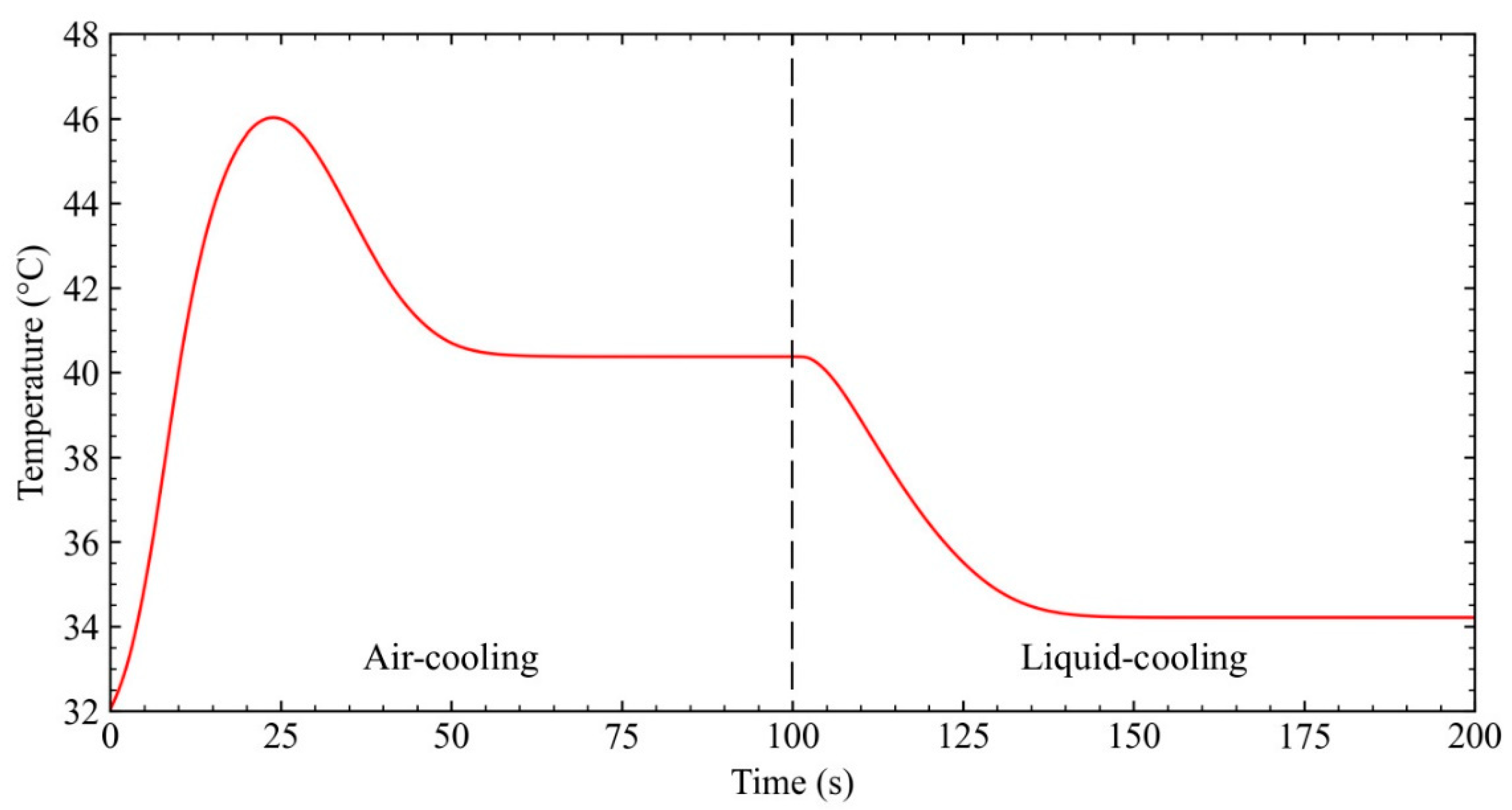
3.3. A Compact Model for the Liquid-Cooled Server
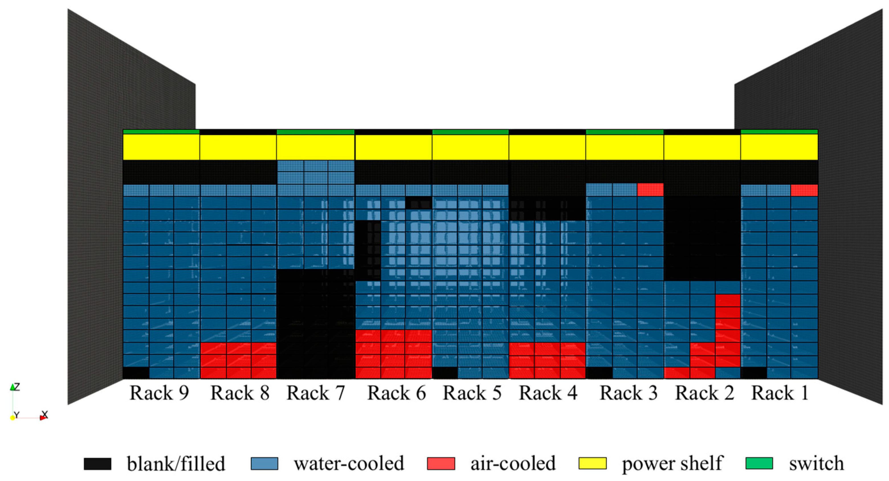
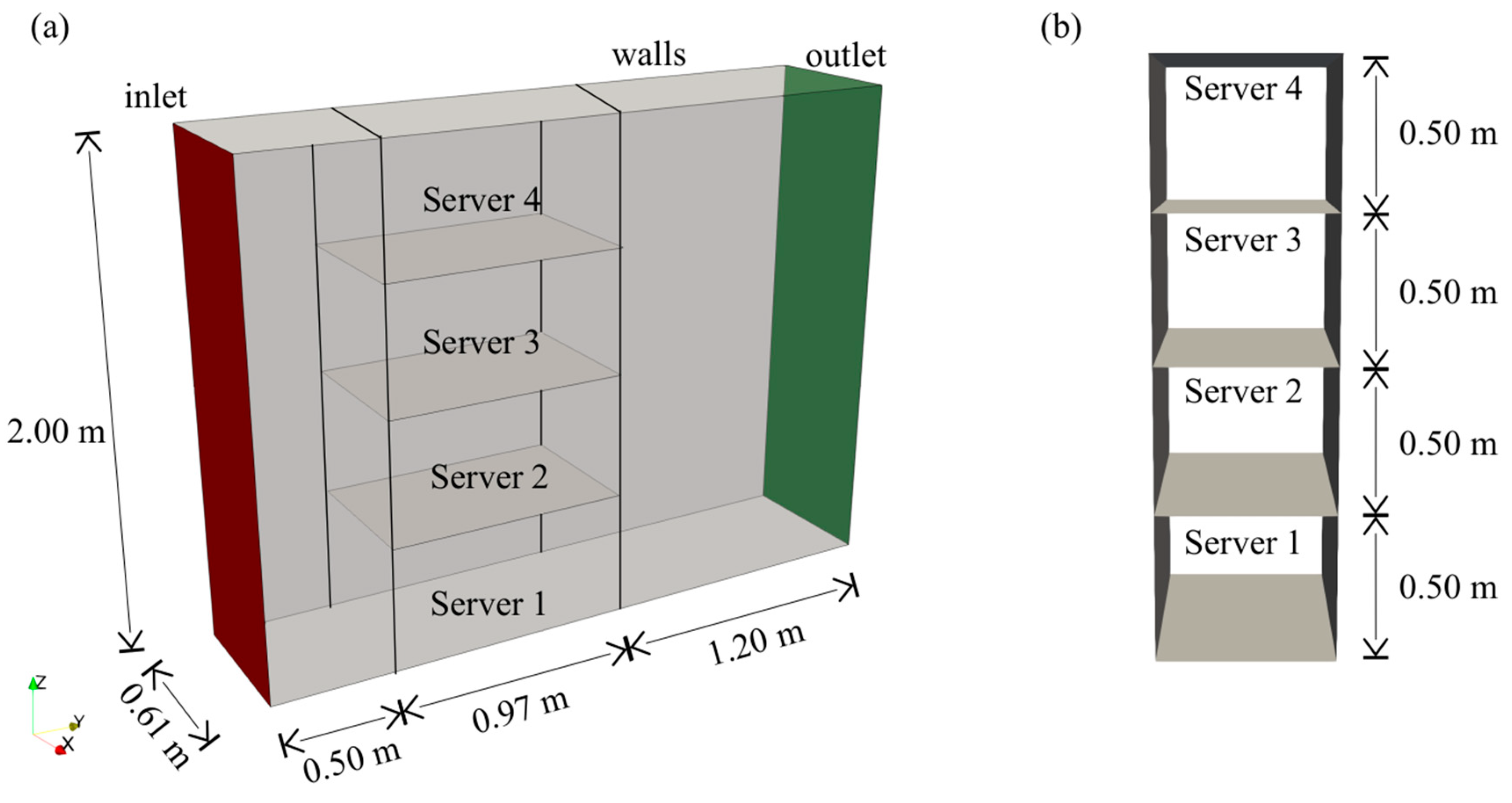
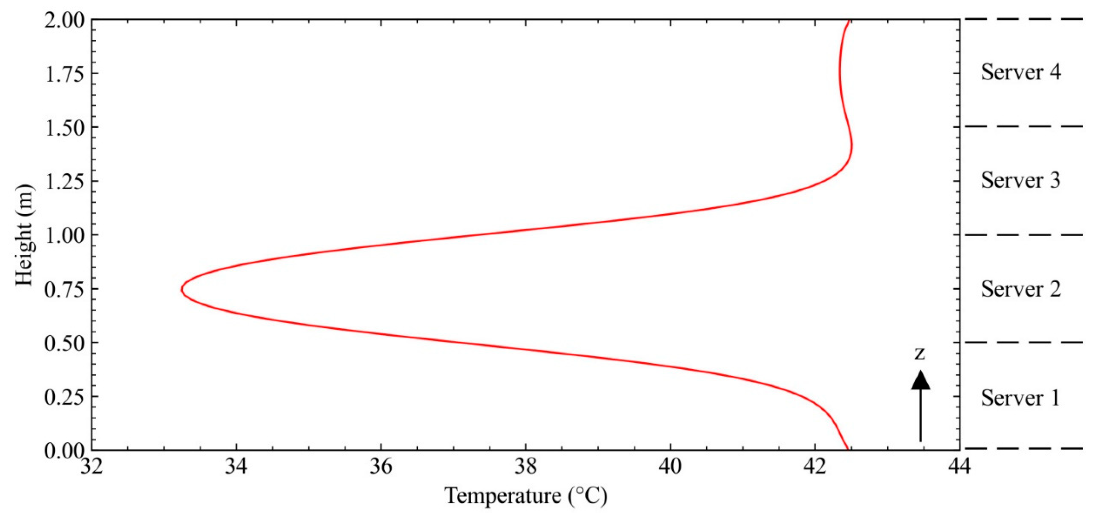
3.4. Thermal Analysis of a Hybrid Cooled Rack
4. Conclusions
Author Contributions
Funding
Data Availability Statement
Conflicts of Interest
References
- Sun, R.; Fu, Q.; Chen, G.; Li, Y.; Wang, S.; Zhang, J.; Fan, Y.; Xia, Y.; Ahuja, N. A Novel Concept Methodology of In-direct Cold Plate Liquid Cooling Design for Data Center in CPU Socket Area. In Proceedings of the 2020 19th IEEE Intersociety Conference on Thermal and Thermomechanical Phenomena in Electronic Systems (Itherm), Orlando, FL, USA, 21–23 July 2020. [Google Scholar]
- Ramakrishnan, B.; Alkharabsheh, S.; Hadad, Y.; Sammakia, B.; Chiarot, P.R.; Seymour, M.; Tipton, R. Experimental characterization of a cold plate used in warm water cooling of data centers. In Proceedings of the 2017 33rd Thermal Measurement, Modeling & Management Symposium (SEMI-THERM), San Jose, CA, USA, 13–17 March 2017. [Google Scholar]
- Gao, T.; Shao, S.; Cui, Y.; Espiritu, B.; Ingalz, C.; Tang, H.; Heydari, A. A study of direct liquid cooling for high-density chips and accelerators. In Proceedings of the 2017 16th IEEE Intersociety Conference on Thermal and Thermomechanical Phenomena in Electronic Systems (ITherm), Orlando, FL, USA, 30 May–2 June 2017. [Google Scholar]
- VanGilder, J.W.; Pardey, Z.; Healey, C.; Zhang, X. A compact server model for transient data center simulations. ASHRAE Trans. 2013, 119, 358–370. [Google Scholar]
- Pardey, Z.M.; Demetriou, D.V.; Erden, H.S.; VanGilder, J.W.; Khalifa, E.Z.; Schmidt, R.R. Proposal for standard compact server model for transient data center simulations. ASHRAE Trans. 2015, 121, 413. [Google Scholar]
- Ibrahim, M.; Bhopte, S.; Sammakia, B.; Murray, B.; Iyengar, M.; Schmidt, R. Effect of thermal characteristics of electronic enclosures on dynamic data center performance. In Proceedings of the ASME 2010 International Mechanical Engineering Congress and Exposition, Vancouver, BC, Canada, 12–18 November 2010. [Google Scholar]
- Manaserh, Y.M.; Tradat, M.I.; Bani-Hani, D.; Alfallah, A.; Sammakia, B.G.; Nemati, K.; Seymour, M.J. Machine learning assisted development of IT equipment compact models for data centers energy planning. Appl. Energy 2015, 305, 117846. [Google Scholar] [CrossRef]
- Ellsworth, M.J., Jr.; Iyengar, M.K. Energy efficiency analyses and comparison of air and water cooled high performance servers. In Proceedings of the International Electronic Packaging Technical Conference and Exhibition, San Francisco, CA, USA, 19–23 July 2009. [Google Scholar]
- Geng, H. Data Center Handbook; John Wiley & Sons: Hoboken, NJ, USA, 2014. [Google Scholar]
- Kadam, S.T.; Kumar, R. Twenty first century cooling solution: Microchannel heat sinks. Int. J. Therm. Sci. 2014, 8, 73–92. [Google Scholar] [CrossRef]
- Ellsworth, M.J.; Goth, G.F.; Zoodsma, R.J.; Arvelo, A.; Campbell, L.A.; Anderl, W.J. An overview of the IBM power 775 supercomputer water cooling system. J. Electron. Packag. 2012, 134, 020906. [Google Scholar] [CrossRef]
- Tuma, P.E. The merits of open bath immersion cooling of datacom equipment. In Proceedings of the 2010 26th Annual IEEE Semiconductor Thermal Measurement and Management Symposium (SEMI-THERM), Santa Clara, CA, USA, 21–25 February 2010. [Google Scholar]
- Garimella, S.V.; Yeh, L.T.; Persoons, T. Thermal management challenges in telecommunication systems and data centers. IEEE Trans. Compon. Packag. Manuf. Technol. 2012, 2, 1307–1316. [Google Scholar] [CrossRef]
- Bar-Cohen, A.; Arik, M.; Ohadi, M. Direct liquid cooling of high flux micro and nano electronic components. Proc. IEEE 2006, 94, 1549–1570. [Google Scholar] [CrossRef]
- Zimmermann, S.; Meijer, I.; Tiwari, M.K.; Paredes, S.; Michel, B.; Poulikakos, D. Aquasar: A hot water cooled data center with direct energy reuse. Energy 2012, 43, 237–245. [Google Scholar] [CrossRef]
- Han, Y.; Tang, G.; Lau, B.L.; Zhang, X. Hybrid micro-fluid heat sink for high power dissipation of liquid-cooled data centre. In Proceedings of the 2017 IEEE 19th Electronics Packaging Technology Conference (EPTC), Singapore, 6–9 December 2017. [Google Scholar]
- Sridhar, A.; Vincenzi, A.; Atienza, D.; Brunschwiler, T. 3D-ICE: A compact thermal model for early-stage design of liquid-cooled ICs. IEEE Trans. Comput. 2013, 63, 2576–2589. [Google Scholar] [CrossRef] [Green Version]
- Carbó, A.; Oró, E.; Salom, J.; Canuto, M.; Macías, M.; Guitart, J. Experimental and numerical analysis for potential heat reuse in liquid cooled data centres. Energy Convers. Manag. 2016, 112, 135–145. [Google Scholar] [CrossRef] [Green Version]
- Rubenstein, B.A.; Zeighami, R.; Lankston, R.; Peterson, E. Hybrid cooled data center using above ambient liquid cooling. In Proceedings of the 2010 12th IEEE Intersociety Conference on Thermal and Thermomechanical Phenomena in Electronic Systems, Vegas, NV, USA, 2–5 June 2010. [Google Scholar]
- Parida, P.R.; Arvind, S.; Vega, A.; Schultz, M.D.; Gaynes, M.; Ozsun, O.; McVicker, G.; Brunschwiler, T.; Buyuktosunoglu, A. Thermal model for embedded two-phase liquid cooled microprocessor. In Proceedings of the 2017 16th IEEE Intersociety Conference on Thermal and Thermomechanical Phenomena in Electronic Systems (Itherm), Orlando, FL, USA, 30 May–2 June 2017. [Google Scholar]
- Gullbrand, J.; Luckeroth, M.J.; Sprenger, M.E.; Winkel, C. Liquid Cooling of Compute System. J. Electron. Packag. 2019, 141, 010802. [Google Scholar] [CrossRef] [Green Version]
- Battaglioli, S.; Lebon, M.; Jenkins, R.; Summers, J.; Sarkinen, J.; Robinson, A.J. Enhancement of an Open Compute Project (OCP) server thermal management and waste heat recovery potential via hybrid liquid-cooling. In Proceedings of the 2022 28th IEEE International Workshop on Thermal Investigations of ICs and Systems, Dublin, Ireland, 28–30 September 2022. [Google Scholar]
- Simon, V.S.; Reddy, L.S.; Shahi, P.; Valli, A.; Saini, S.; Modi, H.; Bansode, P.; Agonafer, D. CFD Analysis of Heat Capture Ratio in a Hybrid Cooled Server. In Proceedings of the ASME 2022 International Technical Conference and Exhibition on Packaging and Integration of Electronic and Photonic Microsystems, Garden Grove, CA, USA, 25–27 October 2022. [Google Scholar]
- Modi, H.; Shahi, P.; Sivakumar, A.; Saini, S.; Bansode, P.; Shalom, V.; Rachakonda, A.V.; Gupta, G.; Agonafer, D. Transient CFD Analysis of Dynamic Liquid-Cooling Implementation at Rack Level. In Proceedings of the ASME 2022 International Technical Conference and Exhibition on Packaging and Integration of Electronic and Photonic Microsystems, Garden Grove, CA, USA, 25–27 October 2022. [Google Scholar]
- Shahi, P.; Agarwal, S.; Saini, S.; Niazmand, A.; Bansode, P.; Agonafer, D. CFD Analysis on Liquid Cooled Cold Plate Using Copper Nanoparticles. In Proceedings of the ASME 2020 International Technical Conference and Exhibition on Packaging and Integration of Electronic and Photonic Microsystems, Virtual Online, 27–29 October 2020. [Google Scholar]
- Watson, B.; Venkiteswaran, V.K. Universal Cooling of Data Centres: A CFD Analysis. Energy Procedia 2017, 142, 2711–2720. [Google Scholar] [CrossRef]
- Wilcox, D.C. Formulation of the k-ω turbulence model revisited. AIAA J. 2008, 46, 2823–2838. [Google Scholar] [CrossRef] [Green Version]
- Eckert, E.R.G.; Soehngen, E. Distribution of heat transfer coefficients around circular cylinders in crossflow at Reynolds numbers from 20 to 500. Trans. ASME 1952, 74, 343–346. [Google Scholar] [CrossRef]
- Jasak, H.; Aleksandar, J.; Zeljko, T. OpenFOAM: A C++ library for complex physics simulations. In Proceedings of the International Workshop on Coupled Methods in Numerical Dynamics, Dubrovnik, Crotia, 19–21 September 2007. [Google Scholar]
- Dogan, A.; Yilmaz, S.; Kuzay, M.; Demirel, E. OpenFOAM cases for the Validation of the CHT Model [Data set]. In Energies; Version 1; Zenodo: Cern, Switzerland, 2023. [Google Scholar]
- Viswanath, D.S.; Natarjan, G. Data Book on the Viscosity of Liquids; Hemisphere Pub. Corp.: New York, NY, USA, 1989. [Google Scholar]
- White, F.M. Viscous Fluid Flow, 3rd ed.; McGraw-Hill: New York, NY, USA, 2006. [Google Scholar]
- Dogan, A.; Yilmaz, S.; Kuzay, M.; Yilmaz, C.; Demirel, E. CFD Modeling of Pressure Drop through an OCP Server for Data Center Applications. Energies 2022, 15, 6438. [Google Scholar] [CrossRef]
- Dogan, A.; Yilmaz, S.; Kuzay, M.; Demirel, E. Development and validation of an open-source CFD model for the efficiency assessment of data centers. Open Res. Eur. 2022, 2, 41. [Google Scholar] [CrossRef]
- Abdelmaksoud, W.A.; Dang, T.Q.; Ezzat Khalifa, H.; Schmidt, R.R. Improved computational fluid dynamics model for open-aisle air-cooled data center simulations. J. Electron. Packag. 2013, 135, 030901. [Google Scholar] [CrossRef]
- Gschaider, B.F. The incomplete swak4Foam reference. Tech. Rep. 2013, 131, 202. [Google Scholar]


| Case | Variable | Value | Unit |
|---|---|---|---|
| - | Pipe inner diameter | 0.0283 | m |
| Pipe outer diameter | 0.0442 | m | |
| Pipe length | 0.0884 | m | |
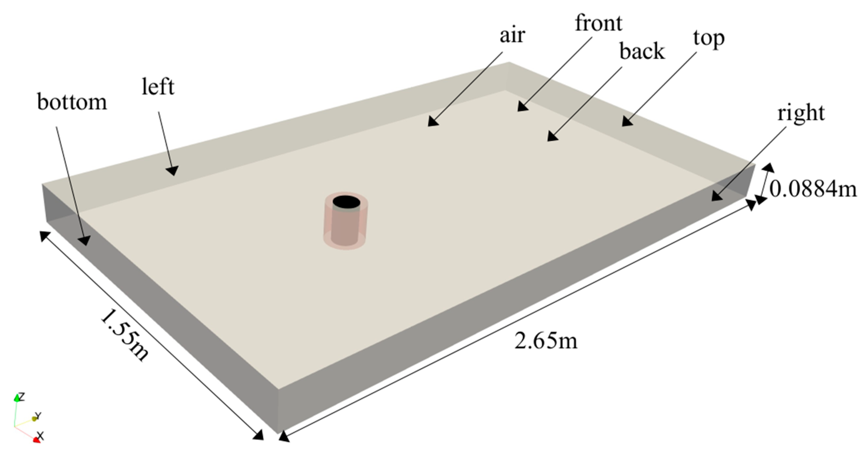
| Size of air domain | 1.55 × 2.65 × 0.0884 | m3 | |
| Free Convection | Water temperature | 315 | K |
| Water velocity | 5 | m/s | |
| Air temperature | 300 | K | |
| Air Prandtl number | 0.7 | - | |
| Raleigh number | 0.86 × 10⁵ | - | |
| Forced Convection | Water temperature | 330 | K |
| Water velocity | 5 | m/s | |
| Air temperature | 300 | K | |
| Air Prandtl number | 0.7 | - | |
| Air velocity | 0.0489 | m/s | |
| Reynolds number | 130 | - |
| Mesh | Number of Cells | Error (%) | |||
|---|---|---|---|---|---|
| Air Region | Water Region | Copper Region | Instantaneous | Time-Averaged | |
| Mesh 1 | 77,488 | 11,344 | 4400 | 5.94 | 4.84 |
| Mesh 2 | 395,296 | 17,344 | 8784 | 4.43 | 4.19 |
| Mesh 3 | 512,320 | 23,200 | 11,120 | 3.18 | 2.41 |
| Mesh 4 | 1,503,488 | 22,288 | 13,616 | 2.73 | 2.70 |
| Region | Inlet Temperature (K) | Outlet Temperature (K) | Temperature Jump (K) | Heat (W) |
|---|---|---|---|---|
| Air | 308.15 | 308.5 | 0.35 | 3.54 |
| Water | 313.15 | 315.03 | 1.88 | 234.04 |
| Server | Power Consumption (W) |
|---|---|
| Server 1 | 3720 |
| Server 2 | 3720 |
| Server 3 | 3840 |
| Server 4 | 3720 |
Disclaimer/Publisher’s Note: The statements, opinions and data contained in all publications are solely those of the individual author(s) and contributor(s) and not of MDPI and/or the editor(s). MDPI and/or the editor(s) disclaim responsibility for any injury to people or property resulting from any ideas, methods, instructions or products referred to in the content. |
© 2023 by the authors. Licensee MDPI, Basel, Switzerland. This article is an open access article distributed under the terms and conditions of the Creative Commons Attribution (CC BY) license (https://creativecommons.org/licenses/by/4.0/).
Share and Cite
Dogan, A.; Yilmaz, S.; Kuzay, M.; Korpershoek, D.-J.; Burks, J.; Demirel, E. Conjugate Heat Transfer Modeling of a Cold Plate Design for Hybrid-Cooled Data Centers. Energies 2023, 16, 3088. https://doi.org/10.3390/en16073088
Dogan A, Yilmaz S, Kuzay M, Korpershoek D-J, Burks J, Demirel E. Conjugate Heat Transfer Modeling of a Cold Plate Design for Hybrid-Cooled Data Centers. Energies. 2023; 16(7):3088. https://doi.org/10.3390/en16073088
Chicago/Turabian StyleDogan, Aras, Sibel Yilmaz, Mustafa Kuzay, Dirk-Jan Korpershoek, Jeroen Burks, and Ender Demirel. 2023. "Conjugate Heat Transfer Modeling of a Cold Plate Design for Hybrid-Cooled Data Centers" Energies 16, no. 7: 3088. https://doi.org/10.3390/en16073088