A Novel Scheme to Allocate the Green Energy Transportation Costs—Application to Carbon Captured and Hydrogen

Abstract

Carbon dioxide (CO₂) and hydrogen (H₂) are essential energy vectors in the green energy transition. H₂ is a fuel produced by electrolysis and is applied in heavy transportation where electrification is not feasible yet. The pollutant substance CO₂ is starting to be captured and stored in different European locations. In Denmark, the energy vision aims to use this CO₂ to be reacted with H₂, producing green methanol. Typically, the production units are not co-located with consumers and thus, the required transportation infrastructure is essential for meeting supply and demand. This work presents a novel scheme to allocate the transportation costs of CO₂ and H₂ in pipeline networks, which can be applied to any network topology and with any allocation method. During the tariff formation process, coordinated adjustments are made by the novel scheme on the original tariffs produced by the allocation method employed, considering the location of each customer connected to pipeline network. Locational tariffs are provided as result, and the total revenue recovery is guaranteed to the network owner. Considering active customers, the novel scheme will lead to a decrease of distant pipeline flows, thereby contributing to the prevention of bottlenecks in the transportation network. Thus, structural reinforcements can be avoided, reducing the total transportation cost paid by all customers in the long-term.

1. Introduction

Around the world, many countries are seeking to reduce the greenhouse gases emitted due to the consumption of carbon-based fossil fuels to deal with the concerns regarding climate change [1,2,3,4,5]. This transition process to a green energy society poses many challenges and questions about the right pathways to be taken [6,7,8]. In addition, the current Ukrainian crisis adds more apprehension and uncertainties regarding global energy resources and their availability in the future [9]. Energy independence, aimed at by countries, requires long-term solutions without fossil fuels through the employment of clean and zero-carbon renewable energy sources [10,11,12]. The substance carbon dioxide (CO₂) has been captured from diverse industrial plants and stored as part of the energy actions related to green climate targets [8,13,14]. Also, hydrogen (H₂) technologies present a strong potential to emerge as an energy ecosystem, having a synergistic integration with solar, wind, hydraulic, nuclear, and other zero-carbon sources [1,15,16]. The substances CO₂ and H₂, possess the capability to be integrated with existing energy infrastructure such as pipeline networks. However, the infrastructure to transport green energy fuels still needs to achieve a cost-effective pathway [6,8,13,14,15].

Considering this context, the work brings as its main contributions the following:

• A significant literature review about regulatory challenges regarding the infrastructure needed for new green energy businesses;
• An integrated framework that allows for the evaluation of a dynamic process with production and consumption entities connected through a pipeline network;
• A novel scheme to allocate transportation costs in pipelines with generic modelling that can be applied with any network topology and with any allocation method;
• Application results considering a pipeline network simulated through several cases, which permits the novel scheme evaluation over an expressive period;
• Comparative analyses illustrating the decrease of distant pipeline flows with the novel scheme employment;
• Provision of future research directions as next steps regarding a broader green energy perspective.

The document is organized as follows. Section 2 presents regulatory challenges with respect to the network infrastructure needed to transport new green energy fuels. Section 3 details the integrated framework presented in the work, which contains the novel scheme as its main contribution, since this represents an original development. Section 4 describes the pipeline network employed in this work and the simulation scenario to generate different cases. Section 5 exhibits the results obtained with a specific discussion regarding each case. Section 6 shows the comparative analyses related to pipeline network flows. Finally, Section 7 contains the main conclusions of the work and points out some future research directions.

2. New Green Energy Fuels: Regulatory Challenges Involved with the Transportation Network Infrastructure

According to [8], the main cost drivers of carbon capture and storage (CCS) are plant size, energy costs, and the costs of CO₂ transportation and storage infrastructure. This conclusion is based on a study made with high-emissions industrial production processes, which need to mitigate a substantial amount of process emissions: cement clinker and lime, raw steel, paper, and basic chemicals such as ethylene and ammonia.

The European Union (EU) energy system utilizes modern techniques for grid balancing [15]. The first is a mix of coupling different sectors and an interconnection of building heating/cooling demand, transport, and the industrial sector. The second technique is the application of long-term storage and discharge technologies. Finally, the third one is the transportation of energy from centres of supply to centres of demand, using smart grid procedures. The basic concept behind the coupling of sectors lies in the direct connection of power generation with other energy demand sectors. This approach deals with two problems: energy is not produced at the location where it is required, and it is not produced at the time it is required. The following technologies can be used as coupling approaches: power to heat and power to gas [15]. Power to heat employs the excess of renewable energy production to supply heating/cooling for buildings or other infrastructure. Power to gas is a more flexible sector coupling option to achieve grid balancing and stabilization. H₂ and CO₂ can play an important role in this approach, as well as the methanol produced from the reaction of both substances. Meanwhile, new opportunities can arise from emerging supply chains, such as, regional green fuel grids [17], coupling of distinct energy sectors, and international shipping of liquid renewable energy carriers.

In [13], CCS is pointed out as an attractive integrated assessment model (IAM) since it provides means to explore the future role of technologies in meeting climate targets. CCS can be integrated into existing energy systems and can accommodate the intermittency of renewable technologies, as well as H₂ can play this role [18]. Moreover, CCS is a viable option for the decarbonisation of emission-intensive industries and can be combined with low-carbon or carbon-neutral bioenergy to generate negative emissions. In the EU and United Kingdom (UK), the CO₂ transportation and storage infrastructure does not exist at the same scale, nor is there an enough investment incentive to induce its deployment [13]. Therefore, in these regions, the key barriers are the lack of infrastructure, with the cost of capture as a secondary barrier. Consequently, the EU and UK regions would be better advised to focus on the deployment of transport and storage infrastructure.

As CCS networks have emerged as a vital CCS deployment factor, the development of shared infrastructure for transportation and storage has become a focus for project developers and policymakers [14]. Shared infrastructure includes all capital equipment required to move CO₂ from capture plants to its ultimate storage locations: pipelines, compression systems, ships, port facilities, and ultimately storage installations where multiple CO₂ sources can be injected in shared wells. These storages will be particularly important over the next years while methanol production remains a technology that is not mature enough and has a high economic cost.

Governments and industrial players perform a key role in CCS infrastructure development. Public support goes beyond technical work and includes supportive regulations to enable a firm legal basis to undertake storage, guidelines for pipeline route development, and government support for early-stage exploration. The continued increase to enable CCS to move to gigatonne scales globally will depend on more pipelines, storage projects, and shipping infrastructure over the coming decades [14]. According to [19], the overall construction cost of CO₂ pipelines is currently high, when a cost-benefit analysis is considered. A CO₂ pipeline infrastructure implementation is needed to develop a framework for economic evaluation of bioenergy with carbon capture and storage (BECCS), CCS, and carbon capture and utilisation (CCU) value chains, in terms of total project and operating costs.

Reference [20] also discusses the importance of incentives to CCS deployment. The retrofit of CCS in pulp and paper industry will increase the production cost in the absence of carbon incentives. As with other sectors, the feasibility of CCS in this industry is strongly dependent on how CO₂ emissions are categorized and incentivized. Furthermore, due to the requirements of mills to be close to the source such as forests, their location is often remote. Therefore, CCS in this sector is often overlooked in terms of network and infrastructure integration. Four different climate pathways to analyse possible CCS attainments in the power sector and in relevant industrial sectors were discussed in [21]. Results highlighted the synergistic effect of sharing common CCS infrastructures among power and major industrial sectors. CCS contributions are mainly found in three industrial sectors, particularly steel, cement, and refineries, but also in the power sector to a lesser extent.

2.1. The European Green Deal

Regarding specifically to the European Green Deal and its implications, reference [22] affirmed that energy demand sectors must be decarbonized in a strong way and the European gas infrastructure should be recognized as a key asset for the European economy’s decarbonization. In [23,24], gas infrastructure companies published visions of a dedicated H₂ pipeline transport network spanning several European countries. For achieving the EU climate neutrality by 2050, the implementation of diverse technologies at a large scale is necessary, including BECCS, CCS, and CCU. Additionally, the industrial electrification, the use of H₂, the electromobility expansion, and low-emissions agricultural practices are cited as important green energy vectors [25,26].

With respect to gas transmission tariff methodologies, the traditional Pro Rata method, also named as Postage Stamp, is discussed in [27]. The principle of this methodology is to treat all network points equally, regardless of their network location. As result, despite being perfectly non-discriminatory, its tariffs are not cost-reflective at all. According to [27], the Pro Rata method is completely transparent, but the lack of any kind of cost-reflectivity is its main drawback. Tariffs must evolve in the light of major future changes, such as, the energy sector decarbonization and the electricity and gas sectors coupling [28]. By ensuring transparent tariff procedures now, the burden to manage future challenges can be reduced in the future. The suitable assessment and the efficient valuation of transmission and transportation assets will be essential for the green energy transition.

The gas transportation cost in Europe is currently covered via entry–exit tariffs, based on charging capacity reservations at both entry and exit points of entry–exit systems [29]. These systems coincide largely with Member States’ territories. This model has supported a smooth evolution from the traditional structure of the European gas industry to a single liberalized European market with an expressive number of stakeholders. Nevertheless, the current tariff methodology has been questioned as the European gas market advances. The allegation is that the methodology may be inadequate to achieve the purpose of a single pan-European market with unbiased gas flows and no barriers to trade.

2.2. The Danish Energy Vision

In Denmark, the utility regulator has set the gas transmission tariffs with the following characteristics: regulatory period of three years, tariff period of one year, and Pro Rata reference price methodology [30]. The allowed or target revenue for the Danish gas year 2019-2020 was DKK 423 million (EUR 56.6 million). This allowed revenue are the needed system costs that must be covered by the tariffs, representing thus the budgeted necessary costs. It is relevant to mention that not only Danish gas market data are presented by [30]. This reference also contains information regarding 20 more European jurisdictions, what provides a broad gas market view in Europe. As Power-to-X (PtX) constitutes a vital strategy of the Danish energy vision, it is expected that costs regarding all infrastructure necessary to deploy this strategy will achieve expressive values over next years.

PtX is considered a strategic solution to the Danish decarbonization process since it can replace the last fossil fuel consumption in industry, shipping, heavy-duty vehicles, and aviation [31]. The Danish strategy, to make PtX a great contributor to solving the energy transition challenges, is composed of four key components:

• An ambitious PtX programme to secure that Denmark’s main strengths regarding PtX are exploited, helping to make Denmark fossil-free;
• Danish PtX efforts, through regulation and subsidies, to establish the structural basis for the PtX industrialization, focusing on production with a view to reduce costs;
• Deployment of frameworks and rules for an international green market, valuing the renewable H₂ and boosting then the international demand for PtX;
• Establishment of transparent governance where the business sector is regularly involved and consulted about future adjustments to the PtX strategy.

The government of Denmark has set ambitious targets to reduce greenhouse gas emissions to achieve the Danish climate neutrality by 2050 [32,33]. This will require the employment of green gases in areas where electrification is not feasible for economic or technological reasons, especially regarding the heavy industry. The green energy transition will have direct consequences on the future of the Danish gas system. In [34], initiatives that must be taken in the Danish gas system towards 2040, to keep a high supply security over the green energy transition, are presented. Initially, the infrastructure must be able to handle a decline in gas consumption, a change in consumer behaviour, and a growth in biogas production. Afterwards, in the slightly longer term, there may arise a need to adjust Denmark’s gas infrastructure to meet the demand for transport and storage of distinct green gases, such as, H₂, CO₂, and methanol.

Based on the literature analysed in this section, we notice that green energy fuels will perform an important role in the energy transition process. Some areas of the electricity system are expected to become overloaded, as expressive green electricity amounts will be generated, without the possibility to be consumed locally. In many of these areas, green gas production is expected to be available. Thus, this production can contribute to provide a better use of renewable energy sources in surplus periods, coupling the sectors of electricity and gas. Similarly, green gas production plants can be planned considering local weather changes. In this way, the heat produced at plants can be coupled with the district heating. Therefore, it is logical that new green gases will require expressive modifications into the actual network infrastructure. In new green energy businesses such as CO₂ and H₂, the needed infrastructure for matching demand and supply will still need to be built, since there are no representative networks in place. We can verify a high degree of freedom regarding the establishment of business rules. In this way, the rules defined will profoundly impact business costs in the long-term, as green business growth rates will be high over the next decades, amplifying the defined rules’ impact.

3. Integrated Framework for Green Energy: Novel Scheme to Allocate Transportation Costs in Pipelines

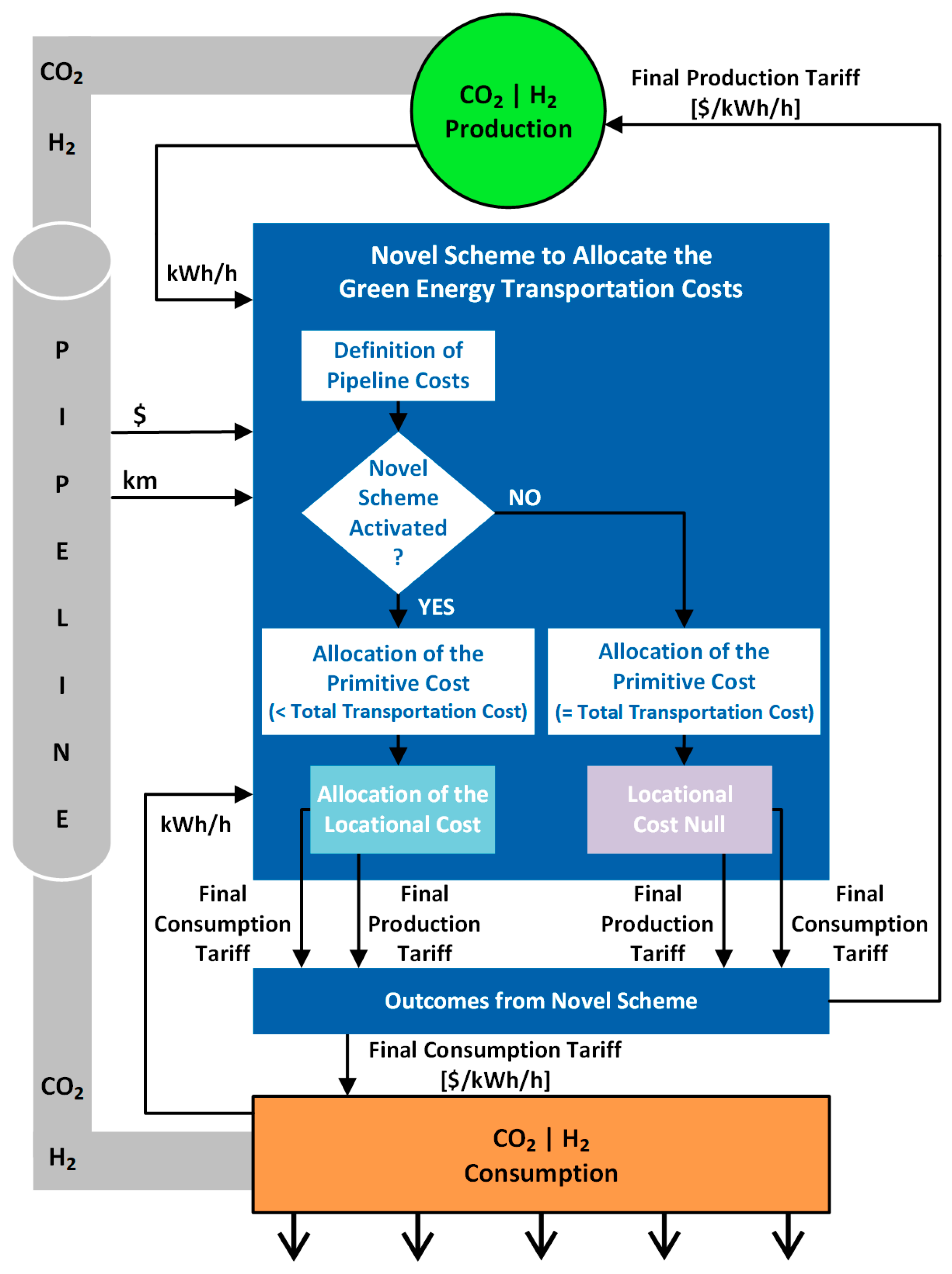
In this work, an integrated framework was developed to allow the analysis regarding the feedback between pipeline transportation capacity tariffs and responses from entities of CO₂|H₂ production and consumption. Figure 1 shows the arrangement of this integrated framework. We can observe that the framework is composed of four parts: a novel scheme to form the transportation capacity tariffs, a CO₂|H₂ production entity, a CO₂|H₂ consumption entity, and a pipeline network as the transportation means employed to connect production and consumption. The novel scheme constitutes an original development, thus being the main contribution of this work. The customer location at each pipeline point was captured by the novel scheme and coordinated adjustments were performed on the original tariffs produced by the allocation method employed in one of its stages. The adjustments were proportional to the distance of each customer regarding the others. Therefore, the novel scheme provides individual economic signals to customers as outcomes and constitutes a valuable flexibility resource for the current green energy transition era.

The novel scheme forms transportation capacity tariffs, in $/kWh/h, through a process constituted of sequential stages, from which it is obtained: the final consumption tariff $PTNU{T}^C\left(i\right)$ and the final production tariff $PTNU{T}^P\left(i\right)$. To execute the stage calculations, only three sets of information are utilized: the CO₂|H₂ production and consumption at each pipeline point in kWh/h, the distance between each pipeline point in km, and the total cost to transport CO₂ and/or H₂ through the pipeline network in $. Then, the final tariffs are employed by CO₂|H₂ production and consumption entities updating their values. Thus, these new production and consumption values are provided to the novel scheme that then updates the transportation capacity tariffs in a dynamic process.

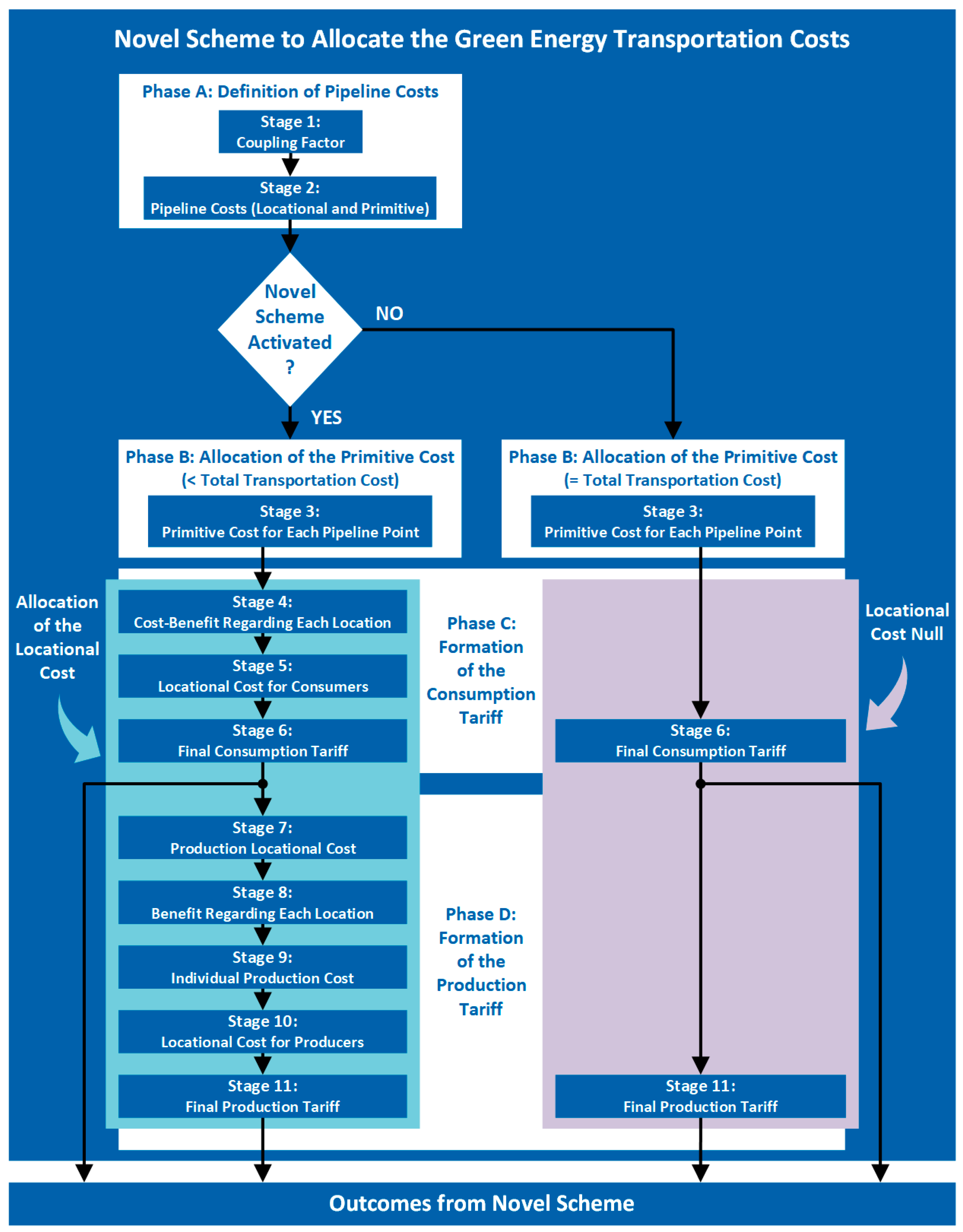
The different stages that constitute the tariff formation process performed by novel scheme can be summarized in four phases, as illustrated by Figure 2.

• Phase A: Definition of Pipeline Costs (Stages 1 and 2);
• Phase B: Allocation of the Primitive Cost (Stage 3);
• Phase C: Formation of the Consumption Tariff (Stages 4–6);
• Phase D: Formation of the Production Tariff (Stages 7–11).

In Phase A, the total transportation cost (TTC), in $, is subdivided into two different costs: locational and primitive. This TCC value corresponds to the total cost that needs to be paid by the set of all pipeline customers, representing thus the pipeline owner revenue. Then, the primitive cost is allocated among pipeline customers by any allocation method in Phase B. Afterwards, the final consumption tariff is formed during Phase C, and the final production tariff is formed in Phase D, through sequential stages. In the following, each stage that composes novel scheme is described in detail.

3.1. Stage 1: Coupling Factor

To subdivide the TTC value in next stage, a coupling factor is calculated:

$$F=\frac{\left({{\displaystyle \sum }}_{i=1}^{N_P}{X}^{+}\left(i_C\right)\right)\times W_F}{N_P\times X_{Total}},$$

(1)

where $F$ is the coupling factor (dimensionless), $N_P$ is the total number of producers, $X^{+}\left(i_C\right)$ is the more distant consumer of the generator i considering the shortest pipeline path in km, $W_F$ is the coupling factor weight (dimensionless), and $X_{Total}$ is the total length of the pipeline network in km. $W_F$ is a nonnegative value ($W_F\ge 0$) that can amplify $F$ ($W_F>1$); attenuate $F$ ($0<W_F<1$); or even cancel $F$ ($W_F=0$), allowing thus the inactivation of novel scheme.

3.2. Stage 2: Pipeline Costs (Locational and Primitive)

Then, with the coupling factor calculated, pipeline costs are obtained:

$$Cos{t}_{Loc}^{Total}=TTC\times F,$$

(2)

$$Cos{t}_{Pri}^{Total}=TTC\times \left(1-F\right),$$

(3)

where $Cos{t}_{Loc}^{Total}$ is the locational cost in $, $Cos{t}_{Pri}^{Total}$ is the primitive cost in $, and $TTC$ represents the total transportation cost also in $. Different regulatory procedures can be applied to determine how much will be the final value to be recovered by the pipeline network owner. The definition of specific criteria to form the TTC value is outside the scope of this work, which focuses on allocating TTC across the pipeline points.

Locational cost only exists if $F$ is not null. It means that if we determine $W_F=0$, we inactivate novel scheme, becoming null locational cost. In this configuration, primitive cost acquires the same total transportation cost value:

$$W_F=0\to F=0\to Cos{t}_{Loc}^{Total}=0\to Cos{t}_{Pri}^{Total}=TTC.$$

(4)

Moreover, the sum of these two costs (locational and primitive) guarantees the full TTC recovery for any $F$:

$$Cos{t}_{Loc}^{Total}+Cos{t}_{Pri}^{Total}=TTC\times F+TTC\times \left(1-F\right)=TTC\times \left(F+1-F\right)=TTC.$$

(5)

3.3. Stage 3: Primitive Cost for Each Pipeline Point

Afterwards, primitive cost obtained previously is allocated to each pipeline point. In this work, we employ Pro Rata method that executes the allocation in a uniform way, since it is the most used reference price methodology in Europe:

$$Cos{t}_{Pri}^C\left(i\right)=\left(\frac{Cos{t}_{Pri}^{Total}}{C_{Total}}\right)\times C_{\%}^{Total}\times C\left(i\right),$$

(6)

$$Cos{t}_{Pri}^P\left(i\right)=\left(\frac{Cos{t}_{Pri}^{Total}}{P_{Total}}\right)\times \left(1-C_{\%}^{Total}\right)\times P\left(i\right),$$

(7)

where $Cos{t}_{Pri}^C\left(i\right)$ is the primitive cost allocated to the consumer i in $, $C_{Total}$ is the total CO₂|H₂ consumption in kWh/h, $C_{\%}^{Total}$ is the cost percentage to be allocated among the consumers (dimensionless) with $0\le C_{\%}^{Total}\le 1$, $C\left(i\right)$ is the consumption at the pipeline point i in kWh/h, $Cos{t}_{Pri}^P\left(i\right)$ is the primitive cost allocated to the producer i in $, $P_{Total}$ is the total CO₂|H₂ production in kWh/h, and $P\left(i\right)$ is the production at the pipeline point i in kWh/h. In the work, it is employed $C_{\%}^{Total}=0.5$ to be allocated the same primitive cost parcel between consumption and production (50–50%). We must mention that this stage may utilize any other allocation method, such as, Contract Path and MW-Mile.

3.4. Stage 4: Cost-Benefit Regarding Each Location

Hereafter, a cost-benefit value for each consumer is calculated considering its location related to the set of all network producers:

$$Cos{t}_{Bene}^{Ex-Ante}\left(i\right)=\frac{Cos{t}_{Loc}^{Total}}{P_{Total}\times X_{Total}}\times \left(\frac{C\left(i\right)}{C_{Total}}\right)\times \left({\displaystyle \sum }_{j=1}^{N_P}P\left(j\right)\times X\left(ji\right)\right),$$

(8)

where $Cos{t}_{Bene}^{Ex-Ante}\left(i\right)$ is the cost-benefit regarding the consumer i in $, $P\left(j\right)$ is the production at the point j in kWh/h, and $X\left(ji\right)$ is the shortest pipeline distance in km between the points j and i. However, this cost-benefit does not guarantee the full TTC recovery.

3.5. Stage 5: Locational Cost for Consumers

A locational cost containing the additional portion necessary for the full TTC recovery is then obtained for each consumer:

$$Cos{t}_{Loc}^C\left(i\right)=Cos{t}_{Bene}^{Ex-Ante}\left(i\right)+\frac{\left(Cos{t}_{Loc}^{Total}-{{\displaystyle \sum }}_{i=1}^{N_C}Cos{t}_{Bene}^{Ex-Ante}\left(i\right)\right)\times N_C\times C\left(i\right)}{N_{PC}\times C_{Total}},$$

(9)

where $Cos{t}_{Loc}^C\left(i\right)$ is the locational cost in $ associated with the consumer i, $N_C$ is the total number of consumers, and $N_{PC}$ is the total number of producers and consumers.

3.6. Stage 6: Final Consumption Tariff

Thus, with the needed costs obtained, $Cos{t}_{Pri}^C\left(i\right)$ and $Cos{t}_{Loc}^C\left(i\right)$, the final consumption tariff is given by:

$$PTNU{T}^C\left(i\right)=\frac{Cos{t}_{Pri}^C\left(i\right)+Cos{t}_{Loc}^C\left(i\right)}{C\left(i\right)},$$

(10)

where $PTNU{T}^C\left(i\right)$ is the pipeline transportation network use tariff in $/kWh/h related to the consumer i.

3.7. Stage 7: Production Locational Cost

To start the production tariff formation process, a general cost is defined as:

$$Cos{t}_{Loc}^P=\frac{Cos{t}_{Loc}^{Total}-{{\displaystyle \sum }}_{i=1}^{N_C}Cos{t}_{Bene}^{Ex-Ante}\left(i\right)}{N_{PC}},$$

(11)

where $Cos{t}_{Loc}^P$ is the locational cost in $ associated with production. We can notice that this cost possesses a general value, having as function the coupling between consumption and production tariff formation processes.

3.8. Stage 8: Benefit Regarding Each Location

Thus, to add an individual character to the formation process, a benefit is established:

$$Ben{e}_{Loc}^P\left(i\right)=Cos{t}_{Loc}^P\times \frac{X_{Total}}{C_{Total}}\times \left({\displaystyle \sum }_{k=1}^{N_C}\frac{C\left(k\right)}{X\left(ik\right)}\right)\times W_B,$$

(12)

where $Ben{e}_{Loc}^P\left(i\right)$ is the individual benefit in $ of the producer i regarding its location, $C\left(k\right)$ is the consumption at the point k in kWh/h, $X\left(ik\right)$ is the shortest pipeline distance in km between the points i and k, and $W_B$ is the benefit weight (dimensionless). $W_B$ is a nonnegative value ($W_B\ge 0$) that can amplify the benefit effect ($W_B>1$); attenuate the effect ($0<W_B<1$); or even cancel all benefits ($W_B=0$).

3.9. Stage 9: Individual Production Cost

Subsequently, the difference between general cost, defined at Stage 7, and individual benefit, established at Stage 8, is employed to calculate:

$$Cos{t}_{Ex-Ante}^P\left(i\right)=\left(Cos{t}_{Loc}^P-Ben{e}_{Loc}^P\left(i\right)\right)\times \frac{P\left(i\right)}{P_{Max}},$$

(13)

where $Cos{t}_{Ex-Ante}^P\left(i\right)$ is the individual production cost in $ associated with the producer i and $P_{MAX}$ is the maximum production value in kWh/h throughout the pipeline network. Nonetheless, this cost does not guarantee the full TTC recovery.

3.10. Stage 10: Locational Cost for Producers

A locational cost for each producer with the additional portion needed for the full TTC recovery is then obtained:

$$Cos{t}_{Loc}^P\left(i\right)=Cos{t}_{Ex-Ante}^P\left(i\right)+\left(\frac{Cos{t}_{Loc}^P\times N_P-{{\displaystyle \sum }}_{i=1}^{N_P}Cos{t}_{Ex-Ante}^P\left(i\right)}{P_{Total}}\right)\times P\left(i\right),$$

(14)

where $Cos{t}_{Loc}^P\left(i\right)$ is the locational cost in $ associated with the producer i.

3.11. Stage 11: Final Production Tariff

Therefore, with the necessary costs obtained, $Cos{t}_{Pri}^P\left(i\right)$ and $Cos{t}_{Loc}^P\left(i\right)$, the final production tariff is calculated:

$$PTNU{T}^P\left(i\right)=\frac{Cos{t}_{Pri}^P\left(i\right)+Cos{t}_{Loc}^P\left(i\right)}{P\left(i\right)},$$

(15)

where $PTNU{T}^P\left(i\right)$ is the pipeline transportation network use tariff in $/kWh/h related to the producer i. This stage ends the tariff formation process performed by novel scheme.

3.12. Synthesis of the Sequential Stages

Table 1. Synthesis of the stages that form novel scheme.

Stage	Main Variables	Set of Input
1	$F$: coupling factor	$X^{+}\left(i_C\right)$: more distant consumer of the generator i $W_F$: coupling factor weight $N_P$: total number of producers $X_{Total}$: total length of the pipeline network
2	$Cos{t}_{Loc}^{Total}$: locational cost $Cos{t}_{Pri}^{Total}$: primitive cost	$TTC$: total transportation cost $F$
3	$Cos{t}_{Pri}^C\left(i\right)$: primitive cost allocated to the consumer i $Cos{t}_{Pri}^P\left(i\right)$: primitive cost allocated to the producer i	$C_{Total}$: total CO2|H2 consumption $C_{\%}^{Total}$: cost percentage to be allocated among the consumers $C\left(i\right)$: consumption at the pipeline point i $P_{Total}$: total CO2|H2 production $P\left(i\right)$: production at the pipeline point i $Cos{t}_{Pri}^{Total}$
4	$Cos{t}_{Bene}^{Ex-Ante}\left(i\right)$: cost-benefit regarding the consumer i	$P\left(j\right)$: production at the point j $X\left(ji\right)$: shortest pipeline distance between the points j and i $Cos{t}_{Loc}^{Total}$; $P_{Total}$; $X_{Total}$; $C\left(i\right)$; $C_{Total}$
5	$Cos{t}_{Loc}^C\left(i\right)$: locational cost associated with the consumer i	$N_C$: total number of consumers $N_{PC}$: total number of producers and consumers $Cos{t}_{Bene}^{Ex-Ante}\left(i\right)$; $Cos{t}_{Loc}^{Total}$; $C\left(i\right)$; $C_{Total}$
6	$PTNU{T}^C\left(i\right)$: pipeline transportation network use tariff related to the consumer i	$Cos{t}_{Pri}^C\left(i\right)$; $Cos{t}_{Loc}^C\left(i\right)$; $C\left(i\right)$
7	$Cos{t}_{Loc}^P$: locational cost associated with production	$Cos{t}_{Loc}^{Total}$; $Cos{t}_{Bene}^{Ex-Ante}\left(i\right)$; $N_{PC}$
8	$Ben{e}_{Loc}^P\left(i\right)$: individual benefit of the producer I regarding its location	$C\left(k\right)$: consumption at the point k  $X\left(ik\right)$: shortest pipeline distance between the points I and k  $W_B$: benefit weight $Cos{t}_{Loc}^P$; $X_{Total}$; $C_{Total}$
9	$Cos{t}_{Ex-Ante}^P\left(i\right)$: individual production cost associated with the producer i	$P_{MAX}$: maximum production value throughout the pipeline network $Cos{t}_{Loc}^P$; $Ben{e}_{Loc}^P\left(i\right)$; $P\left(i\right)$
10	$Cos{t}_{Loc}^P\left(i\right)$: locational cost associated with the producer i	$Cos{t}_{Ex-Ante}^P\left(i\right)$; $Cos{t}_{Loc}^P$; $N_P$; $P_{Total}$; $P\left(i\right)$
11	$PTNU{T}^P\left(i\right)$: pipeline transportation network use tariff related to the producer i	$Cos{t}_{Pri}^P\left(i\right)$; $Cos{t}_{Loc}^P\left(i\right)$; $P\left(i\right)$

synthesizes the main variables and the respective set of input with regard ach one of the stages that form novel scheme, described over previous sections.

We can verify that the stages are processed in a sequential way. It means that new variables (one or two) are defined at each stage. Moreover, the set of input utilized in each stage is always composed of information previously known or calculated.

4. Pipeline Network and Simulation Scenario

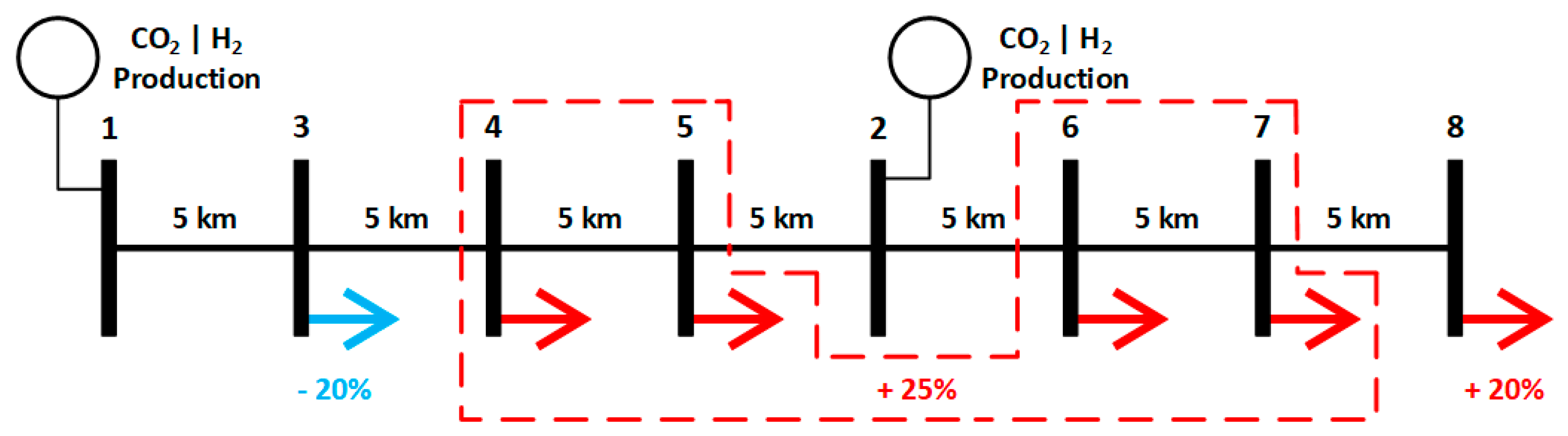
The pipeline network employed in this work is composed of eight points, from which two are points of CO₂|H₂ production (1 and 2) and six are points of CO₂|H₂ consumption (3–8), as shown by Figure 3.

Consumption located at Point 3 is declined by 20% every instant of time. On the other hand, consumption at Point 8 is grown by 20% every instant. These consumers present this behaviour regardless the tariff values at their pipeline points. Thus, they can be defined as inactive customers, or unresponsive customers because they do not respond to the tariffs. Other consumers (Points 4–7) constitute a set that grows its total consumption by 25% every instant. This total consumption growth is subdivided across four points considering their tariff values. Therefore, these customers can be called as active, or responsive.

The growth of consumption is subdivided among the four active points in a way inversely proportional to their tariffs. It means that points with the lowest tariffs receive the highest consumption growths in the following proportion: first (cheapest)—40%; second—30%; third—20%; and fourth (most expensive)—10%. If two or more active points present the same tariff value, the consumption growth becomes equal for these points, keeping the proportions of other active points unchanged.

Regarding production, both producers located at Points 1 and 2 are active, or responsive customers, because they respond to the tariff values. These producers counterbalance the pipeline network consumption growth, increasing their production. The increases are inversely proportional to their tariffs with the following proportion: first (cheapest)—60% and second (most expensive)—40%. If these two active points present the same tariff value, the production increase becomes equal for both points, that is, 50% for each one.

The TTC value to be allocated throughout this pipeline network is given by:

$$TTC=\left({10}^3\right)\times \left(X_{Total}\right).$$

(16)

As we can see in Figure 3, $X_{Total}=35$. Therefore, for all instants of time that compose the simulations, TTC presents $35,000 as its value.

The algorithms of all stages, detailed along the previous section, were developed on a Matlab platform. Moreover, pipeline flows with the absence of network losses are employed to allow comparative analyses regarding the results obtained with only Pro Rata method and with the novel scheme. To simulate the pipeline flows, the computation package Matpower version 7.0 was utilized, a consolidated open-source tool that runs on Matlab offering performance and robustness in network simulations.

5. Results for Each Pipeline Point

Firstly, this section presents the results obtained with only Pro Rata method, which corresponds to determine $W_F=0$ in Stage 1 to become null the locational cost value (novel scheme inactivated). Therefore, in this configuration named as Option 1, the primitive cost value becomes the total transportation cost.

Afterwards, the results obtained with novel scheme are described. This configuration is named Option 2 with $W_F\ne 0$, thus allocating the locational cost through the stages in Phases C and D. The discussion regarding the application results is made over the section to provide to readers a description of each case in detail.

5.1. Option 1: Results Obtained with Only Pro Rata Method

The results provided by only Pro Rata method are presented in this section. First, CO₂|H₂ production and consumption values regarding each pipeline network point, are shown. Later, the transportation capacity tariffs obtained are exhibited.

The results are composed of outcomes related to different instants of time. The first instant, named as 0, constitutes the base case scenario. From this instant, 10 new cases are originated (from instant 1 to 10) in a sequential process, what provides a substantial period to analyse the dynamic behaviour related to all parts that constitute the integrated framework developed in the work.

Table 2. CO₂|H₂ production and consumption values for the pipeline network between the instants of time 0 and 5 with $W_F=0$.

Point	CO2|H2 Production and Consumption [kWh/h]
1	30.0000	35.0000	41.6400	50.2400	61.2200	75.0800
2	30.0000	35.0000	41.6400	50.2400	61.2200	75.0800
3	10.0000	8.0000	6.4000	5.1200	4.1000	3.2800
4	10.0000	12.5000	15.6200	19.5200	24.4000	30.5000
5	10.0000	12.5000	15.6200	19.5200	24.4000	30.5000
6	10.0000	12.5000	15.6200	19.5200	24.4000	30.5000
7	10.0000	12.5000	15.6200	19.5200	24.4000	30.5000
8	10.0000	12.0000	14.4000	17.2800	20.7400	24.8800
	0	1	2	3	4	5
	Instant of Time

illustrates CO₂|H₂ production and consumption values from the instant 0 to the instant 5.

Table 3. CO₂|H₂ production and consumption values for the pipeline network between the instants of time 6 and 10 with $W_F=0$.

Point	CO2|H2 Production and Consumption [kWh/h]
1	92.4800	114.2650	141.4600	175.3700	217.6150
2	92.4800	114.2650	141.4600	175.3700	217.6150
3	2.6200	2.1000	1.6800	1.3400	1.0700
4	38.1200	47.6500	59.5600	74.4500	93.0600
5	38.1200	47.6500	59.5600	74.4500	93.0600
6	38.1200	47.6500	59.5600	74.4500	93.0600
7	38.1200	47.6500	59.5600	74.4500	93.0600
8	29.8600	35.8300	43.0000	51.6000	61.9200
	6	7	8	9	10
	Instant of Time

exhibits the correspondent values between the instants 6 and 10.

Regarding active producers, we can notice an equal production growth at Points 1 and 2 during the whole period. Related to consumers, we verify that Point 3 decreases its consumption at a constant rate since it is an inactive customer. It means that its behavior is not related to its tariff values. The same happens with Point 8 that increases its consumption with the same growth rate. The group formed by Points 4–7 is composed of active customers, who respond to the tariffs. We observe that all components of this group increase their respective consumption in an equal rate over the period.

We can also observe that the results exhibited by Table 3 maintain the same behavior when compared to the values illustrated by Table 2. The active producers at Points 1 and 2 grow their production with an equal proportion, as well as the active consumers at Points 4–7. The inactive consumers located at Points 3 and 8 keeps their respective rates of consumption decrease and increase along the period.

Table 4. Final production and consumption tariffs for each point and the total transportation cost between the instants of time 0 and 5 with $W_F=0$.

Point	Final Production and Consumption Tariff [$/kWh/h]
1	291.6667	250.0000	210.1345	174.1640	142.9271	116.5424
2	291.6667	250.0000	210.1345	174.1640	142.9271	116.5424
3	291.6667	250.0000	210.1345	174.1640	142.9271	116.5424
4	291.6667	250.0000	210.1345	174.1640	142.9271	116.5424
5	291.6667	250.0000	210.1345	174.1640	142.9271	116.5424
6	291.6667	250.0000	210.1345	174.1640	142.9271	116.5424
7	291.6667	250.0000	210.1345	174.1640	142.9271	116.5424
8	291.6667	250.0000	210.1345	174.1640	142.9271	116.5424
TTC [$]	35,000	35,000	35,000	35,000	35,000	35,000
	0	1	2	3	4	5
	Instant of Time

displays final production and consumption tariffs from the instant 0 until the instant 5 and

Table 5. Final production and consumption tariffs for each point and the total transportation cost between the instants of time 6 and 10 with $W_F=0$.

Point	Final Production and Consumption Tariff [$/kWh/h]
1	94.6151	76.5764	61.8549	49.8945	40.2086
2	94.6151	76.5764	61.8549	49.8945	40.2086
3	94.6151	76.5764	61.8549	49.8945	40.2086
4	94.6151	76.5764	61.8549	49.8945	40.2086
5	94.6151	76.5764	61.8549	49.8945	40.2086
6	94.6151	76.5764	61.8549	49.8945	40.2086
7	94.6151	76.5764	61.8549	49.8945	40.2086
8	94.6151	76.5764	61.8549	49.8945	40.2086
TTC [$]	35,000	35,000	35,000	35,000	35,000
	6	7	8	9	10
	Instant of Time

shows the corresponding tariffs between the instants 6 and 10.

We can verify that the tariffs of all pipeline network points present the same value over the whole period. This is an intrinsic characteristic of Pro Rata method that provides always uniform tariffs, regardless the application conditions. It means that the Pro Rata method does not provide any economic signal to pipeline customers.

5.2. Option 2: Results Obtained with Novel Scheme

The results obtained with the novel scheme activation are described in this section. Firstly, CO₂|H₂ production and consumption values, related to each pipeline network point, are exhibited. Afterwards, the transportation capacity tariffs calculated by novel scheme are exposed.

Regarding the parameters utilized by the novel scheme, the results described were obtained with the following settings: $W_F=0.25$ (Stage 1) and $W_B=1.0$ (Stage 8) for all instants of time.

Table 6. CO₂|H₂ production and consumption values for the pipeline network between the instants of time 0 and 5 with $W_F=0.25$ and $W_B=1.0$.

Point	CO2|H2 Production and Consumption [kWh/h]
1	30.0000	34.0000	39.3200	46.2100	54.9900	66.0900
2	30.0000	36.0000	43.9800	54.3100	67.4900	84.1300
3	10.0000	8.0000	6.4000	5.1200	4.1000	3.2800
4	10.0000	13.5000	17.2500	21.9400	27.8000	35.1200
5	10.0000	13.5000	18.5000	24.7500	32.5600	42.3300
6	10.0000	12.0000	14.5000	17.6200	21.5300	26.4100
7	10.0000	11.0000	12.2500	13.8100	15.7600	18.2000
8	10.0000	12.0000	14.4000	17.2800	20.7400	24.8800
	0	1	2	3	4	5
	Instant of Time

shows CO₂|H₂ production and consumption from the instant 0 to the instant 5.

Table 7. CO₂|H₂ production and consumption values for the pipeline network between the instants of time 6 and 10 with $W_F=0.25$ and $W_B=1.0$.

Point	CO2|H2 Production and Consumption [kWh/h]
1	80.0200	97.4600	119.2300	146.3800	180.2100
2	105.0300	131.1800	163.8300	204.5400	255.2700
3	2.6200	2.1000	1.6800	1.3400	1.0700
4	44.2700	55.7100	70.0100	87.8900	110.2400
5	54.5400	69.8000	88.8700	112.7100	142.5100
6	32.5100	40.1400	49.6800	61.6000	76.5000
7	21.2500	25.0600	29.8300	35.7900	43.2400
8	29.8600	35.8300	43.0000	51.6000	61.9200
	6	7	8	9	10
	Instant of Time

illustrates the correspondent values between the instants 6 and 10.

Related to producers, we can verify a higher production growth at Point 2, which is closer to consumption, than the production located at Point 1. These results show the novel scheme effectiveness, since the benefit calculated in its Stage 8 aims to provide tariff discounts to producers closer to consumption. In relation to consumers, Point 3 reduces its consumption at a constant rate as it is an inactive customer. It means that its behaviour is not related to its tariff values. The same occurs with Point 8, which grows its consumption with the same growth rate. The group formed by Points 4–7 is composed of active customers responding to the tariffs. Regarding this group, we noticed the biggest consumption growth at Point 5 and the second highest growth is verified at Point 4. Moreover, the third-highest growth occurs at Point 6 and the smallest growth happens at Point 7. Thus, we notice a direct proportion between consumption growths and their respective locations throughout the pipeline network. The active consumers closer to the production become bigger, since they are incentivized to acquire this behaviour by the novel scheme through the tariffs provided by it. Therefore, the results shown confirm the conceptual ideas that constitute the novel scheme basis.

Table 7 in comparison to Table 6 illustrates that production and consumption, regarding all pipeline network points, keep their correspondent behaviours until the last instant of time. Thus, this result reveals that the tariffs provided by novel scheme related to active customers (Points 1, 2, 4–7) are stable.

Table 8. Final production and consumption tariffs for each point and the total transportation cost between the instants of time 0 and 5 with $W_F=0.25$ and $W_B=1.0$.

Point	Final Production and Consumption Tariff [$/kWh/h]
1	265.9557	230.5620	195.6527	163.3690	134.8638	110.4581
2	242.9729	206.5452	172.6215	142.6470	116.9319	95.3100
3	313.9881	269.7919	227.3773	188.9871	155.5271	127.1385
4	313.9881	269.4275	226.7777	188.2714	154.7832	126.4247
5	313.9881	269.0630	226.1781	187.5556	154.0392	125.7109
6	328.8690	281.4537	236.2970	195.7222	160.5846	130.9408
7	343.7500	294.2088	247.0156	204.6046	167.8738	136.8845
8	358.6310	306.9639	257.7342	213.4870	175.1630	142.8281
TTC [$]	35,000	35,000	35,000	35,000	35,000	35,000
	0	1	2	3	4	5
	Instant of Time

exposes final production and consumption tariffs from the instant 0 until the instant 5 and

Table 9. Final production and consumption tariffs for each point and the total transportation cost between the instants of time 6 and 10 with $W_F=0.25$ and $W_B=1.0$.

Point	Final Production and Consumption Tariff [$/kWh/h]
1	89.9839	73.0305	59.1212	47.7754	38.5571
2	77.3851	62.6567	50.6341	40.8609	32.9398
3	103.4379	83.8784	67.8617	54.8168	44.2278
4	102.7858	83.3025	67.3647	54.3951	43.8745
5	102.1337	82.7265	66.8677	53.9734	43.5211
6	106.3065	86.0557	69.5249	56.0960	45.2180
7	111.1315	89.9608	72.6791	58.6403	47.2682
8	115.9564	93.8659	75.8333	61.1845	49.3185
TTC [$]	35,000	35,000	35,000	35,000	35,000
	6	7	8	9	10
	Instant of Time

displays the correspondent tariffs between the instants 6 and 10.

Regarding the active producers located at Points 1 and 2, we perceive that the tariff at Point 2 maintains a lower value compared to Point 1, because Point 2 is closer to network consumption. This tariff characteristic explains the bigger production growth verified at Point 2, which was shown by the previous tables. Related to consumers, we observe a direct relationship between each tariff and its proximity to network production. At the instant of time 0, when the producers present the same value, the tariffs at Points 3, 4, and 5 are equal since their distance to the overall production is the same. Over the next instants, the tariff at Point 5 becomes the smallest because the producer at Point 2 gets bigger than the producer at Point 1. As a consequence, the tariff at Point 4 becomes the second lowest and the tariff at Point 3 the third lowest. With respect to Points 6–8, we notice that the tariff at Point 8 is the biggest, since the instant 0, as this point is always the most distant from production. The second highest consumption tariff is verified at Point 7 and the third highest tariff at Point 6. This set of results demonstrates the novel scheme’s efficiency on its tariff formation process, as the tariff values possess a direct relationship with the position of each customer in the pipeline network.

Table 9 confirms the results exposed in Table 8, since the correspondent behaviours of all outcomes are kept the same over time. This shows the stability of the tariff formation process performed by the novel scheme, as its capability to provide assertive results in a dynamic running process is demonstrated. We must mention that TTC in Table 8 and Table 9 retains the same value, as previously explained. This value corresponds to the sum of each tariff value multiplied by its value of production or consumption, representing thus the total pipeline owner revenue. The recovery of this value is always guaranteed by the novel scheme, regardless of its configuration.

6. Pipeline Network Flows: Comparative Analyses

Comparative analyses are presented over this section considering the pipeline network flows related to tariffs provided by only Pro Rata method (Option 1) and by novel scheme (Option 2). First, pipeline flow outcomes regarding the employment of tariffs provided by only the Pro Rata method and by the novel scheme are exhibited together in graphs. Later, absolute differences between the pipeline flow outcomes are exposed graphically to allow a better evaluation of the results.

6.1. Flow Outcomes Regarding the Options 1 and 2

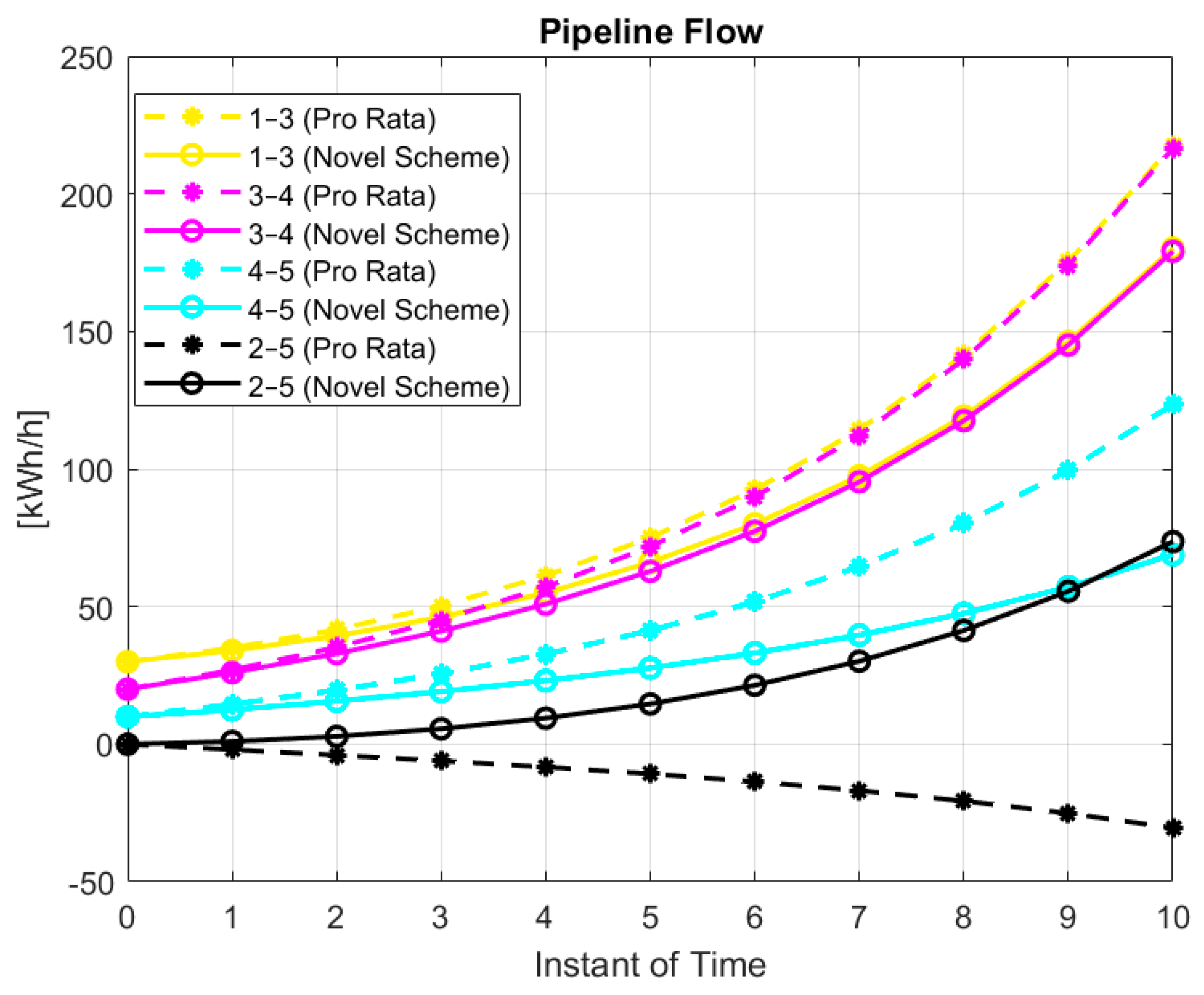
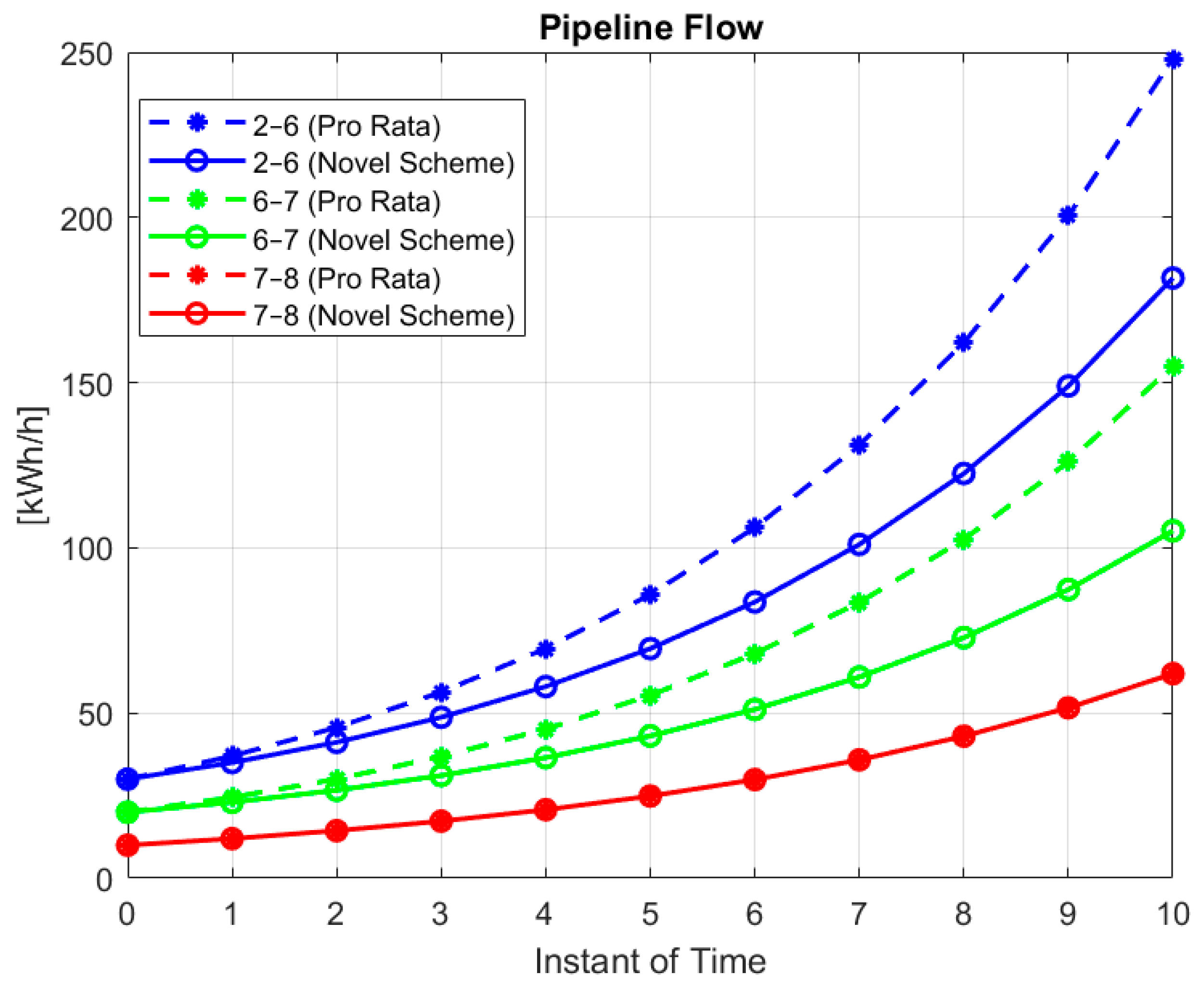
Figure 4 and Figure 5 exhibit pipeline network flows obtained from applying the tariffs provided by only the Pro Rata method ($W_F=0$ in Stage 1) and by the novel scheme ($W_F=0.25$). The flow values related to Pro Rata tariffs are represented by dashed lines and the flow values regarding novel scheme tariffs are represented by full lines.

With the employment of tariffs provided by the novel scheme, we can notice a decrease in the following flows: 1–3, 3–4, 4–5, 2–6, and 6–7. The flow 7–8 keeps the same value, as the consumer located at Point 8 corresponds to the pipeline network end. The flow 2–5 has inverted its direction with a final value higher than the value obtained with only the Pro Rata method. However, this higher value obtained with the novel scheme has a low magnitude when compared to other pipeline flows. These flow behaviours, exhibited by Figure 4 and Figure 5, represent the great contribution of novel scheme in decreasing distant pipeline flows, avoiding then network bottlenecks.

6.2. Absolute Differences between the Pipeline Flow Outcomes

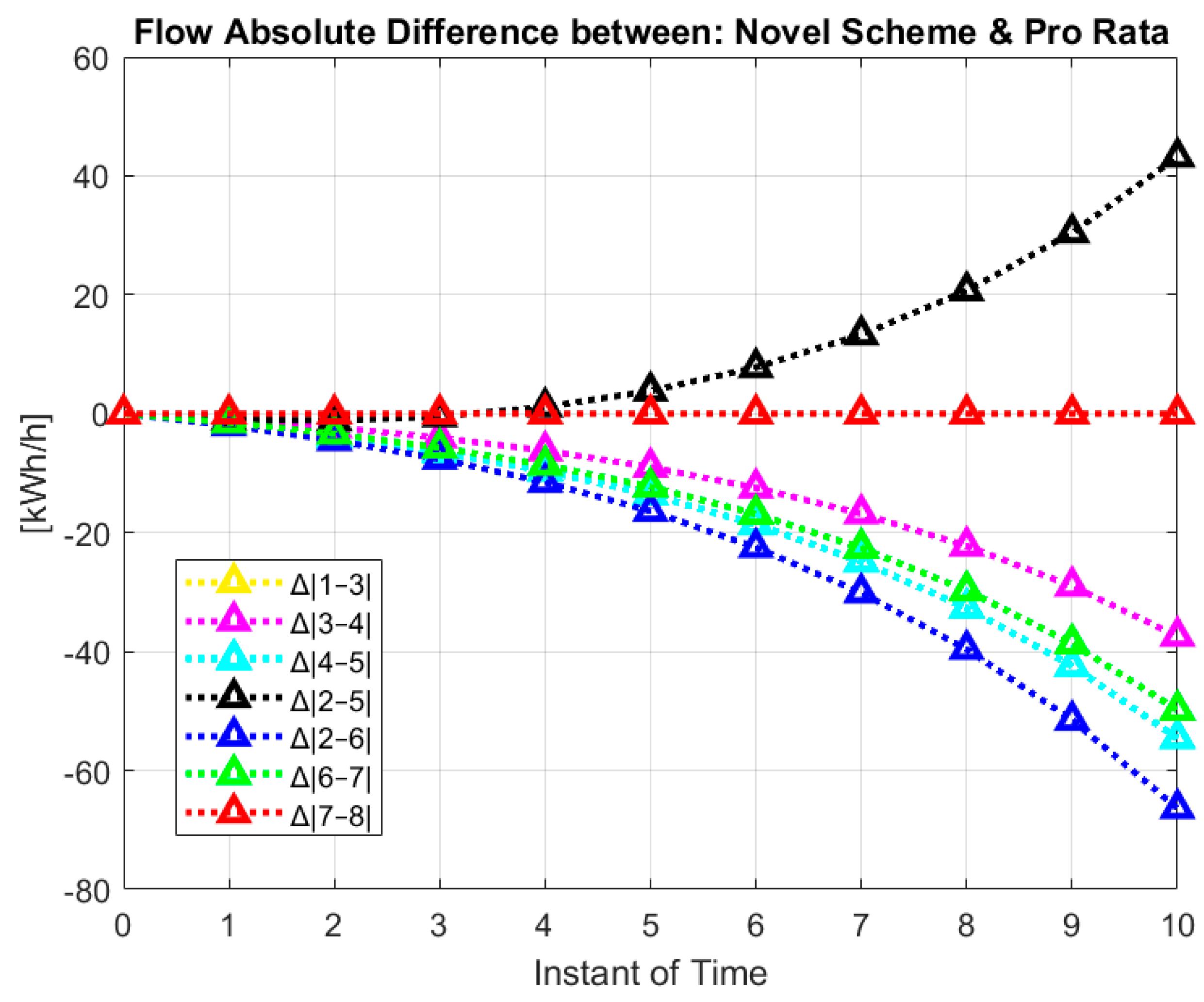
To allow a better visualization of the results presented by Figure 4 and Figure 5, absolute differences between the pipeline flow outcomes obtained with the novel scheme and with only the Pro Rata method are shown in Figure 6. These absolute differences grant readers a direct comparative analysis between the two sets of outcomes.

We can verify the growth of the flow 2–5 that inverts its direction, the maintenance of the flow 7–8, and the decrease of the other flows: 1–3, 3–4, 4–5, 2–6, and 6–7. It is important to mention that the differences regarded the flow 1–3 are identical to those related to the flow 3–4.

Therefore, these results clarify and confirm the efficiency of the novel scheme developed in this work, because distant pipeline flows are decreased and production becomes closer to consumption. In this way, customers are incentivized to adopt behaviours that indirectly prevent bottlenecks, what can postpone, and even avoid, network structural reinforcements. It means that this novel scheme accomplishes its purpose as a regulatory set of rules: stakeholders are incentivized by its rules to improve their individual behaviours taking the system to better planning and operational conditions, which reduces the overall business cost.

7. Conclusions and Future Directions

This work presented a novel scheme to allocate transportation costs of CO₂ and H₂ in pipeline networks, reflecting the location of each customer regarding the set of all others. The novel scheme possesses generic modelling that allows its employment with any allocation method, always guaranteeing the revenue recovery to the pipeline owner. We can verify that the novel scheme also has parameters that permit its tuning, which reveals its flexibility, since it can be applied with any topology network and with any transportation cost.

Novel scheme can be also applied in real pipeline networks independently of the physical losses that occur inside the pipes. Moreover, there is no specific requirement concerning the type of substance is transported by the pipeline. In this work, we are considering the transportation of CO₂ and H₂, as substances that have been considered important energy vectors for new green fuel markets in Europe. However, any substance may be considered in the pipeline.

The consumption location at each pipeline point is captured by novel scheme and coordinated adjustments are performed on the original tariffs produced by the allocation method employed in Stage 3. The adjustments are proportional to the distance of each consumer regarding the producers. As result, the consumers closer to producers get lower tariffs. In terms of production, the location of each producer related to all consumers is apprehended by novel scheme, similarly to consumption. Thus, the producers located closer to consumers obtain cheaper tariffs.

From the results exposed, we can extract important findings regarding the action of this novel scheme. The consumption efficiency is increased, as consumption tariffs reflect consumer locations across the system. So, consumers are incentivized to grow their consumption at points closer to production, which takes to a decrease of distant pipeline flows when active customers, who respond to the tariffs, are considered in the network. Similarly, production gets closer to consumption if active producers are connected to the network, growing their production at points with the cheapest tariffs. Thus, distant flows are decreased throughout the network, what contributes to avoid pipeline bottlenecks.

Another natural consequence as result from the novel scheme application is the reduction of losses in a pipeline network, linked to the decrease of distant pipeline flows. This result is not shown explicitly in this work because losses are not considered in the simulations performed for obtaining the flow values. However, this outcome can be extrapolated as transportation losses regarding any substance in a network has direct relationship with the distances from emitting points to receiver points.

The novel scheme presented over this work comprehends the first development of a broader research regarding new green energy markets. As for future research directions, we can point out the following pathway:

• Assessment of network bottlenecks in actual pipeline infrastructures with the novel scheme application to verify its performance and robustness in face of real data;
• Addition of novel scheme in an aggregated expansion planning to evaluate its efficiency in decreasing structural reinforcements needed to attend growing demands from active pipeline customers;
• Analysis of pipeline losses due to the intrinsic energy deterioration in movements related to the transport of substances between one point to another in networks;
• Proposal of techniques to balance production and consumption of green fuels, as well as to quantify the transportation losses related to a real network;
• Formation of actual values regarding total costs in network infrastructures dedicated to transport green fuels;
• Study of how to make an adequate transition between incipient green markets to more mature phases with interregional networks connecting distant locations;
• Investigation of distinct strategies to incentivize the economic efficiency amongst market participants to reduce the overall cost in new green energy businesses;
• Establishment of suitable stakeholders, entities, and the concerned rules that will constitute the new green market architectures, such as regulatory agencies, commercialization chambers, system operators, sectorial actors, regulatory principles, market mechanisms, price formulations, technical standards, planning expansion guidelines, and reliability criteria.

These new green energy businesses are being planned and developed to achieve the climate targets established by many countries around the world. Therefore, the presence of regulatory and market procedures that guarantee the fairness among customers and promote the market efficiency, through clear rules, is essential. Only with effective procedures can new businesses be incentivized by regulation to expand their infrastructures in a way that the overall costs may be reduced. In this perspective, the novel scheme presented in this work was shown to be apt to contribute to this intent.