1. Introduction
Clean and low carbon energy is the trend of global energy development and the internal requirement of high-quality energy development. In the context of carbon neutrality, the development of energy will undergo profound changes. As a green and clean energy source, nuclear energy has the advantages of high energy density, non-intermittency, and less constraints from natural conditions. In particular, it is important to reduce the use of traditional fossil energy, reduce carbon emissions, and achieve carbon neutrality [
1].
While vigorously developing nuclear energy, ensuring nuclear safety is the primary prerequisite [
2]. For nuclear power systems, the energy source is the nuclear reactor, in which nuclear fission reaction occurs. Compared with traditional thermal power plants, the particularity of nuclear power plants is not only reflected in the complexity of nuclear power systems, but also in the risk of radioactive material leakage after its accidents [
3,
4]. Therefore, a reliable shielding design is particularly important [
5]. In the event of an accident in a nuclear power plant, operators are required to make timely and accurate judgments. Since the complexity of nuclear power plants and unpredictability of accidents are beyond the basis for design, it is very important to design an optimization system with high reliability and strong applicability [
6]. It is of great practical significance to use auxiliary decision techniques to support the operator’s activity under the accident condition, reduce the possibility of the operator making false judgments, and to avoid severe accidents.
With society’s increasing attention to the nuclear power industry, people’s requirements for nuclear safety are also increasing. Fault diagnosis technology plays an important role in the field of nuclear power plant fault diagnosis. Fault diagnosis methods can be broadly divided into quantitative and qualitative analysis methods, among which common quantitative analysis methods include neural networks, support vector machines, rough set theory, etc. The neural network-based fault diagnosis method can handle nonlinear problems, has parallel computing capabilities, and does not require diagnostic and inference rules; it can learn by mapping between the input and output of samples to obtain a training model. The support vector machine method can achieve better performance with less data and avoid overtraining. Cao et al. combined a support vector machine (SVM) with principal component analysis (PCA) to establish a three-layer fault classification model, and simulated three faults in small pressurized water reactors (SPWRs). The experimental results showed that the method had rapidity and high accuracy [
7]. Zio et al. proposed a fault classification method for nuclear power plants based on support vector machines (SVMs). This method combined single-class support vector machines and multi-class support vector machines into a hierarchical structure to classify boiling water reactor feedwater system faults [
8]. Rough set does not need additional information and prior knowledge. Mu et al. proposed a method based on neighborhood rough set to learn and diagnose the training sets of typical faults in nuclear power plants. The results showed that the method can quickly and accurately diagnose fault types [
9]. Xu et al. proposed a fault diagnosis method for nuclear power plants based on support vector machines (SVMs) and rough sets (RSs). This method used rough sets to simplify the data, and then used support vector machines for fault classification [
10].
Qualitative analysis methods include expert system, fuzzy logic, etc. Zhang et al. solved the nuclear power plant fault diagnosis problem with a frequency-based on-line expert system (FBOLES) that accurately detected abnormal signals in all 33 faults simulated [
11]. Mwangi et al. discussed the adaptive neuro-fuzzy inference system (ANFIS) based on the fuzzy logic method. The small-break loss-of-coolant accident of Qinshan I Nuclear Power Plant was used for modeling, and the model had good prediction ability and high sensitivity [
12]. The advantages and disadvantages of various methods are listed in
Table 1.
In order to improve the safety of nuclear power plants, assist operators in fault identification and fault analysis, help operators to make corresponding operations more quickly and accurately in the event of an accident, and to avoid more serious accidents, we need to continuously develop and update the fault diagnosis technology of nuclear power plants. This paper innovatively proposes the SSA-CNN-LSTM model to solve the fault diagnosis problem of nuclear power plants.
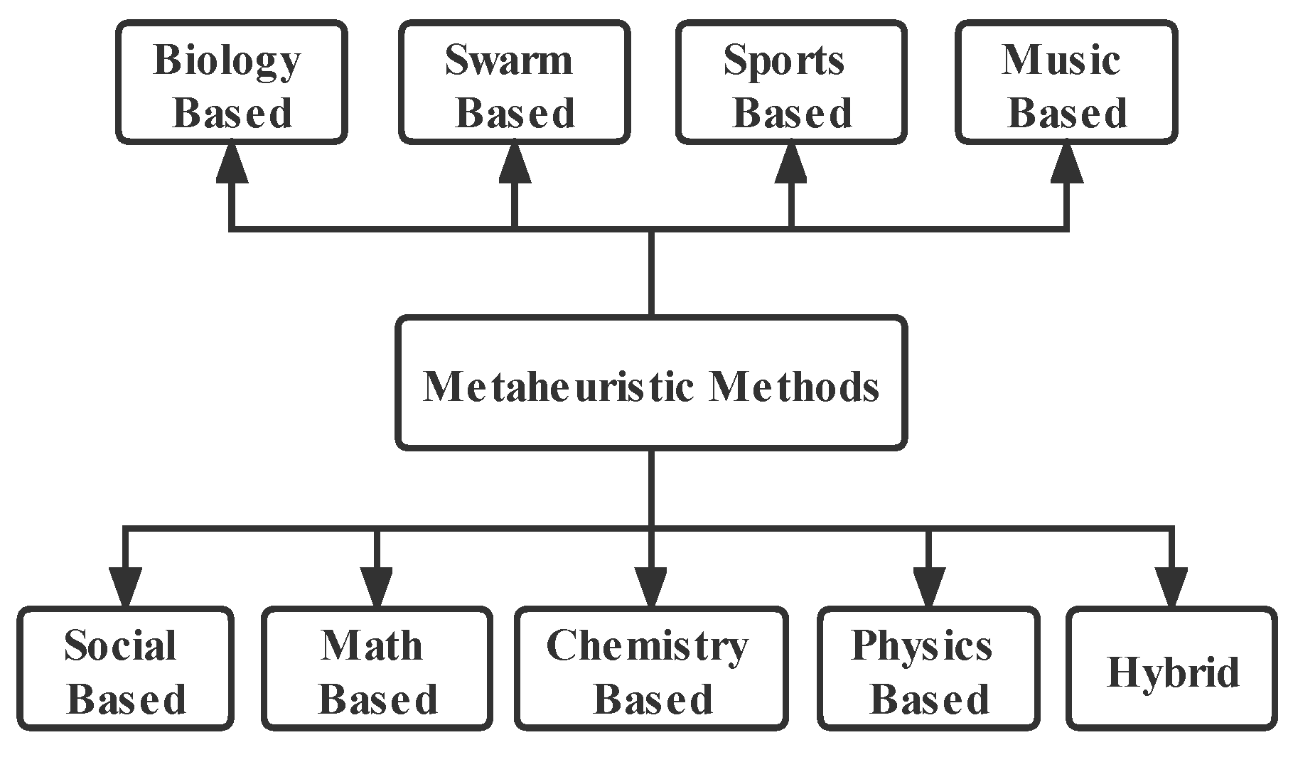
Many fault diagnosis methods have been developed, but improving the accuracy of the model, finding more suitable optimization algorithms, and improving the generalization ability of the model are still the main directions of the research on fault diagnosis methods. In recent years, there have been many researches on metaheuristic algorithms. The metaheuristic algorithm is an algorithm based on intuitive or empirical construction, which can give a feasible solution to the proposed problem. The meta-heuristic strategy adopted by meta-heuristic optimization algorithm is usually a general heuristic strategy, which can be widely used in various fields. Many metaheuristic algorithms are inspired by phenomena in nature. The literature [
13] details nine categories of metaheuristic algorithms and they are biology-based, swarm-based, sports-based, music-based, social-based, math-based, physics-based, chemistry-based, and hybrid methods, as shown in
Figure 1.
People have constructed corresponding biology-based optimization algorithms based on biological behaviors or phenomena, such as invasive weed optimization (IWO) [
14], photosynthetic algorithm [
15], etc. Swarm-based intelligent optimization algorithms that have been built based on the group behavior of animals in nature include the firefly algorithm [
16,
17], bat algorithm [
18], gray wolf optimization algorithm [
19], ant lion optimization algorithm [
20], whale optimization algorithm [
21], etc. In accordance with the physical principles or phenomena, physics-based optimization algorithms have been constructed, such as the simulated annealing algorithm [
22], black hole algorithm [
23], etc. There are also others such as the social-based imperialist competitive algorithm [
24], music-based harmony search [
25], chemistry-based chemical-reaction-inspired metaheuristic for optimization [
26], etc.
Various metaheuristic algorithms are widely used in various fields, such as in computers, industry, medicine, economics, biology, etc. Optimization algorithms are also widely used in the field of nuclear engineering to solve problems. Amm et al. used the ant colony optimization algorithm to solve the nuclear core fuel reload optimization problem [
27]. Khoshahval F et al. studied the application of particle swarm optimization and genetic algorithm in the nuclear fuel loading pattern problem and proved the effectiveness of the algorithm [
28], etc.
In this paper, we combined the advantages of the convolutional neural network (suitable for processing complex data) and the long short-term memory neural network (suitable for processing time series data) to form the CNN-LSTM model, which was used to solve the problem of nuclear power plant fault diagnosis, with a classification accuracy that could reach 95.16%. We then used the sparrow search algorithm to optimize some parameters in the CNN-LSTM model to obtain the SSA-CNN-LSTM model. The experimental results show that the model which was optimized by the sparrow search algorithm is better than the CNN-LSTM model in performance, and proves the accuracy and feasibility of the SSA-CNN-LSTM model.
The fault diagnosis method proposed in this paper can help operators reduce human errors in the event of an accident and reduce the pressure on operators resulting from the accidents, which is of great significance for improving the safety of nuclear power plants. Compared with the traditional fault diagnosis method, the fault diagnosis method based on machine learning has the advantages of fast processing of large amounts of data, analysis and extraction of effective information, and good stability. As a result, in the fault diagnosis technology, the fault diagnosis technology based on machine learning method has received more and more attention. Compared with traditional machine learning methods, SSA is added to automatically optimize some parameters of the model to obtain the optimal model; this can improve the classification accuracy of the model. In addition, the model with SSA has the characteristics of fast convergence.
The rest of this paper is organized as follows.
Section 2 introduces the basic principles of the CNN, the LSTM neural network and the sparrow search algorithm, and the construction of the CNN-LSTM and SSA-CNN-LSTM models.
Section 3 presents the experimental data, the experimental analysis, and the experimental results.
Section 4 presents the conclusion.
2. Methodology
2.1. Convolutional Neural Network (CNN)
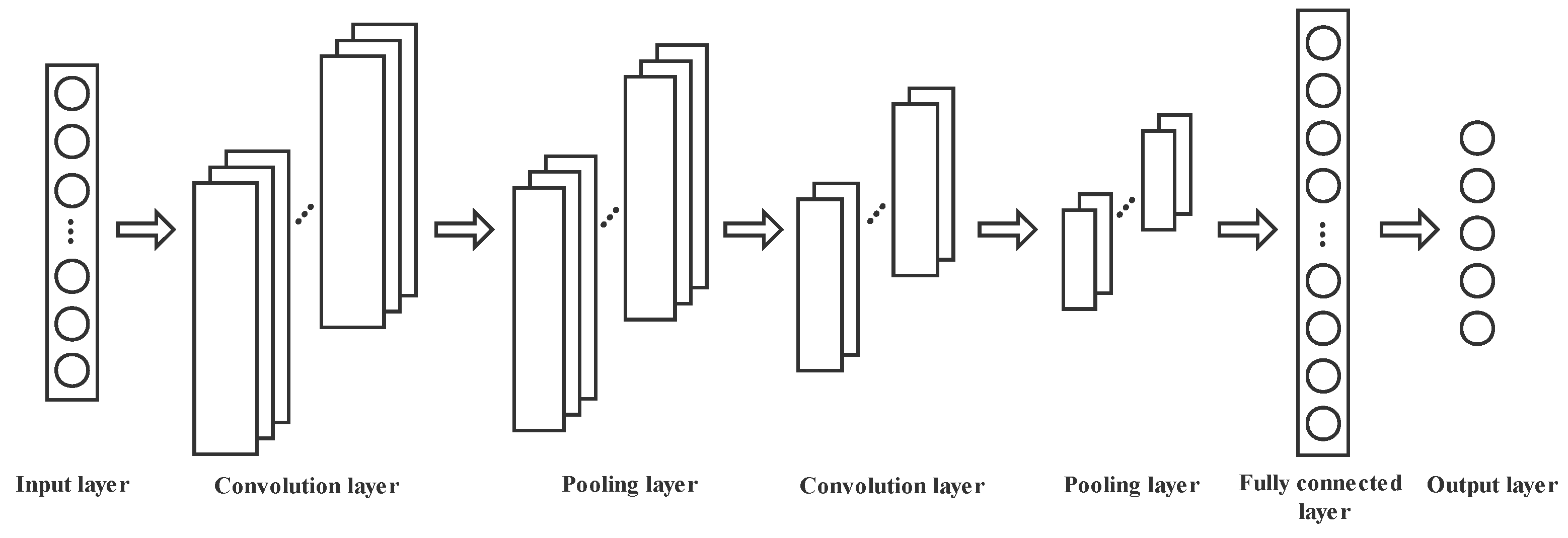
The CNN is a feedforward neural network including convolution computation. The core of the CNN is the convolution kernel. The convolution layer uses the convolution kernel to extract data characteristics. Each neuron in each layer of the CNN characteristic mapping is only related to a small part of the neurons in the previous layer. In the convolution layer operation, the CNN greatly reduces the number of parameters and improves the model training speed by means of local connection of neurons and convolution kernel weight sharing. The structure of the CNN is usually composed of the convolution layer, pooling layer, and full connection layer. The convolution layer is composed of several characteristic graphs obtained by a convolution operation, as shown in
Figure 2. The formula of the convolution layer is shown in Formula (1):
where
represents the number of layers.
represents the
th neuron of layer
.
represents the number of neurons connected between the previous layer and the current layer.
is the weight.
is the bias.
The pooling layer is behind the convolution layer, and is used to compress the model, thus improving the robustness and calculation speed of the model and preventing the occurrence of overfitting to a certain extent.
2.2. Long Short-Term Memory (LSTM) Neural Network
The LSTM neural network introduces the concept of gating units based on the traditional recurrent neural network. When time series data is transferred between units in the implicit layer, it controls the degree of memory and forgetting of the previous and current data in the time series data through controllable gates such as forgetting gates, input gate, and output gate, so that the neural network has the function of long short-term memory. The LSTM neural network has good analysis ability for time series data, and it effectively improves the gradient disappearance and gradient explosion of recurrent neural networks.
The forget gate (
) is calculated by the hidden state of the last moment (
) and the input value of the current moment (
) through the sigmoid activation function layer. The hidden state at the last moment (
) and the input value at the current moment (
) get the input gate (
) through the sigmoid activation function layer, and the candidate cell state (
) through the tanh activation function layer. The current cell state (
) is calculated from the last cell state (
), the new cell state (
), and the input gate (
). The output gate (
) is calculated from the hidden state of the last moment (
) and the input value of the current moment (
). The output gate (
) and the current cell state (
) are calculated to obtain the current hidden state (
), as shown in
Figure 3.
The input gate is used to control the extent to which the current calculation state is updated to the memory cell. The input gate is calculated as shown in Equations (2) and (3).
where
is the input,
is the hidden state,
,
,
,
are the weight matrix and
,
are the bias.
The forget gate is used to control the extent to which the state of the input and current calculation is updated to the memory unit. The forgetting gate calculation formula is shown in (4):
where
is the input,
is the hidden state,
,
are the weight matrix, and
is the bias.
The state is deleted and updated by the forget gate and the input gate. The state calculation formula is shown in (5):
The output gate is used to control the input and the current output depending on the degree of the current memory unit. The output gate calculation formula is shown in (6) and (7):
where
is the input,
is the hidden state,
,
are the weight matrix, and
is the bias.
2.3. CNN-LSTM Model
LSTM neural networks solve the problem of gradient explosion and gradient disappearance in traditional recurrent neural networks. Usually, a LSTM neural network is used to process time series data and predict classification. This paper attempts to use a LSTM neural network to learn the time series data of nuclear power plants and classify the types of nuclear power plant accidents.
Due to the complexity and diversity of nuclear power plant operation data, complex data will increase the training time of the neural network and affect the final classification results. However, a CNN is suitable for processing a large number of high-dimensional and non-linear data [
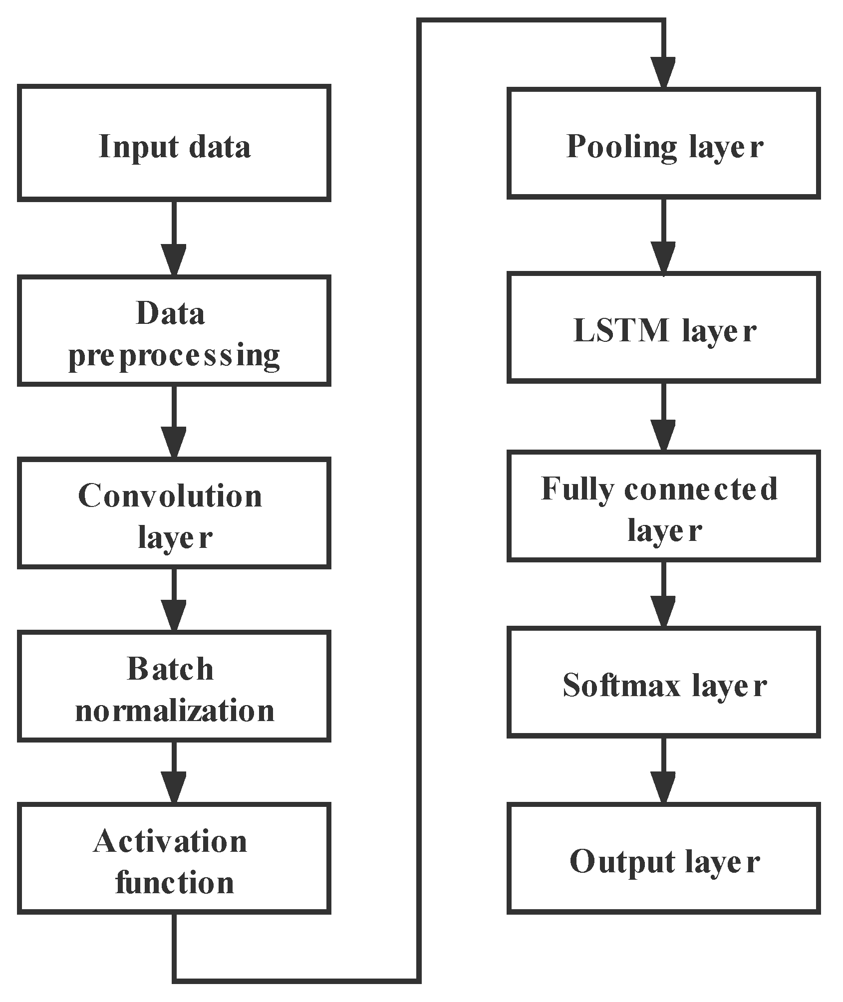
29]. After a series of dimensionality reduction and feature extraction processing such as the CNN layer, batch normalization layer, activation function layer, and pooling layer, the operation data of nuclear power plants not only greatly reduce the number of parameters and retain the important features in the original data, but also improve the learning efficiency of the subsequent LSTM neural network and the fault diagnosis accuracy of the overall model. Therefore, this paper proposes the addition of a convolutional neural network (CNN) before the LSTM neural network to reduce the dimension of the data, thereby forming a CNN-LSTM model. The structure of the CNN-LSTM model is shown in
Figure 4. The data input goes through the convolution layer, batch normalization layer, activation function layer, pooling layer, LSTM layer, fully connected layer, softmax layer, in turn, and finally outputs the results.
2.4. SSA-CNN-LSTM Model
In the above, the CNN-LSTM model was constructed to deal with the fault classification problem of nuclear power plants. However, in the process of constructing the model, it was found that there were many hyperparameters in the neural network, such as the number of neurons, learning rate, number of neural network layers, epoch, etc. The learning rate and the number of hidden layer neurons need to be manually debugged according to experience, and the setting of these two parameters will also have a greater impact on the accuracy of the final results. Therefore, it is of great significance to select an optimization algorithm that can automatically optimize the hyperparameters to improve the accuracy of model classification.
The sparrow search algorithm is a group intelligence optimization technique based on sparrow foraging and anti-predation behaviors [
30]. It has a good search ability in solving optimization problems and has strong parallelism and stability. Therefore, SSA is selected to optimize the parameters of the CNN-LSTM model.
The behavior of sparrows is idealized and corresponding rules are formulated. The foraging process of sparrows can be abstracted as the producer and the scrounger. The producers are responsible for finding food in the population and providing a foraging area and direction for the entire sparrow population, while the scroungers receive food from the producers.
The location update of the producer can be expressed as shown in Formula (8):
where
is the current epoch,
.
is the max number of epochs.
represents the location information in the
th dimension of the
th scrounger.
and
represent the early warning value and safety value, respectively.
is a random number.
is a random number subject to normal distribution.
is a matrix of all 1.
When , this means there is no danger around at this time, and the scroungers can search in a wide range. If , this indicates that there is a danger at this time and an alarm is issued. At this time, the population is transferred to a safe place.
The location update of the producer can be expressed as shown in Formula (9):
where
is the optimal position occupied by the producer, and
is the worst position.
denotes a matrix of
. Each element is 1 or −1 and
. When
, this indicates that the
th scrounger with a low fitness value did not receive food and was in a very hungry state. At this time, the producer needs to find new places to feed.
In case of danger, some sparrows will display anti predatory behavior, and its location update can be expressed as shown in Formula (10):
where
is the current global optimal position. As a step control parameter,
is a random number subject to the normal distribution with mean value of 0 and variance of 1.
is a random number.
is the fitness value of the current sparrow individual.
and
are the global worst and best fitness values, respectively.
is the smallest constant.
When , this indicates that the sparrows are vulnerable to predator attacks. indicates that this position is the best position. When , this shows that the sparrow is in danger. indicates the direction of the sparrow’s movement.
The relevant rules of the sparrow search algorithm are as follows:
- (1)
The producers are responsible for the task of searching for objects and paths.
- (2)
When the sparrow finds a predator, it will send an alarm to the population. When the alarm value is less than that of the safe value, the signal will be ignored, and when the alarm value is beyond that of the safe value, the population will go into play to escape to a safe area.
- (3)
The identities of the producers and scroungers of the sparrow population are not fixed, but the proportion of the discoverers is fixed.
- (4)
The lower the fitness value of the scroungers in the population, the worse their position will be in the population, indicating that they will need to forage elsewhere.
- (5)
Scroungers can find producers that provide better foraging areas in the sparrow population.
- (6)
When the population is threatened, individuals at the edge will find a safe position and move, while individuals at other positions in the population move randomly.
The fitness function is an important part of the optimization problem, which can measure the performance of the algorithm. The sparrow search algorithm calculates the fitness value once at each population update to determine the classification accuracy of the sparrow search algorithm. The fitness value in this paper is the reciprocal of the classification accuracy, and the classification accuracy is the ratio of the same number of predicted values and actual values to the total number of samples. The classification accuracy expression is shown in Formula (11):
where
is the same number of predicted values and actual values,
is the total number of samples, and the fitness function is shown in Formula (12):
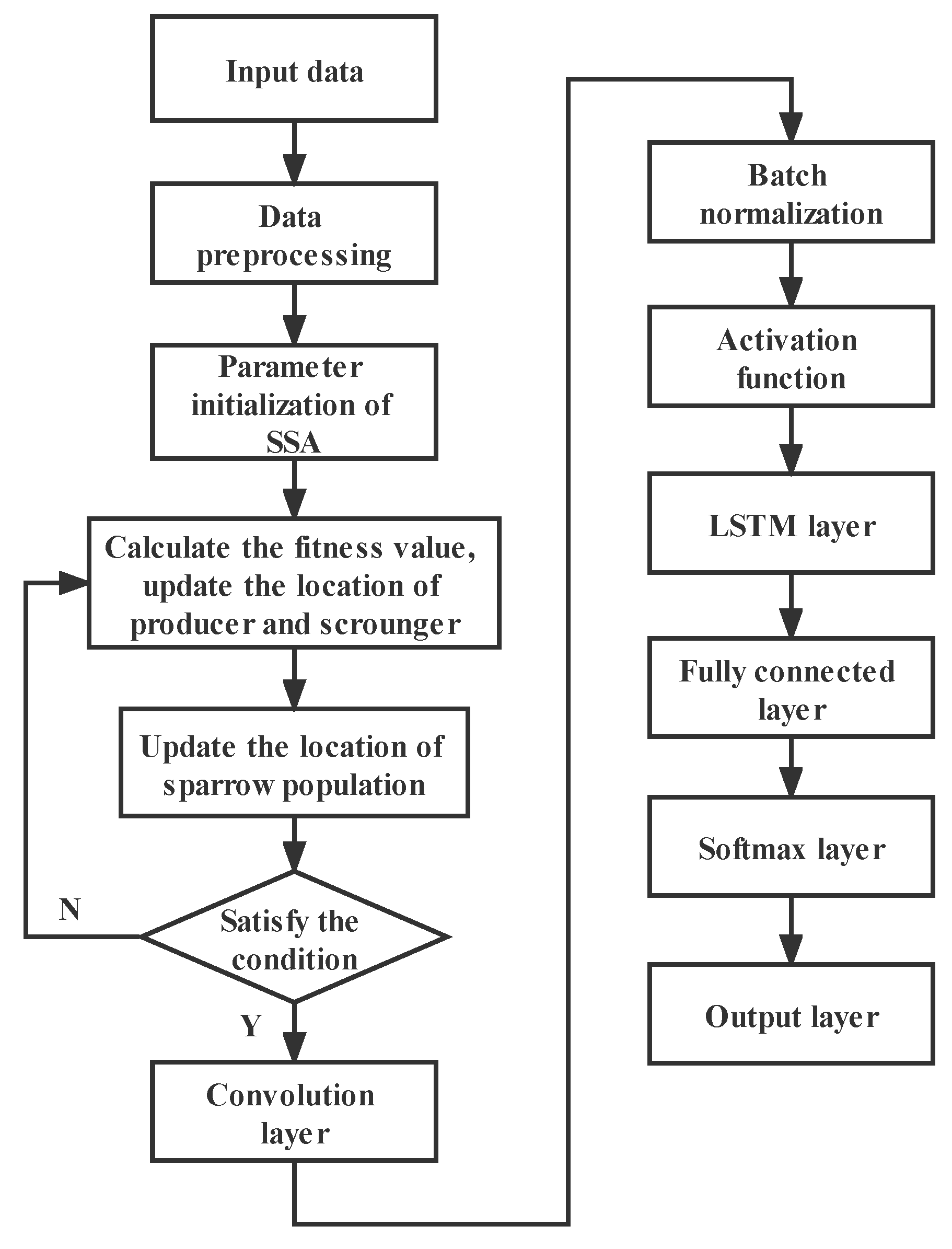
Combining the sparrow search algorithm and CNN-LSTM models, the SSA-CNN-LSTM model was constructed. The structure of the SSA-CNN-LSTM model is as follow:
- (1)
Data preprocessing: data labeling, data set division, data normalization, and data format conversion.
- (2)
SSA parameter initialization: setting the number of sparrows as n, the number of producers as PD, the number of sparrows sensing danger as SD, the safety threshold as ST, and the alarm value as R2.
- (3)
Calculating the fitness value, and updating the location of producer and scrounger.
- (4)
According to the anti-predation behavior, updating the location of the sparrow population.
- (5)
Inputting the data into the CNN network, the data through the CNN layer, batch normalization layer, activation function layer, and average pooling layer.
- (6)
The data enters the LSTM neural network and is inputted to the full connection layer and softmax layer through the LSTM layer.
- (7)
Output results.
Based on the above model structure construction steps, the SSA-CNN-LSTM model flow chart is shown in
Figure 5:
The learning rate and the number of hidden layer nodes are important parameters of the neural network, which have a great influence on the training results. The learning rate controls the learning progress of the model. An excessive learning rate will make the network difficult to converge and linger near the optimal value. A learning rate which is too low will make the network converge very slowly and increase the time to find the optimal value. In this paper, the initial learning rate of the LSTM neural network was set to 0.0035. The number of hidden layer nodes has a certain influence on the performance of the model. Too many hidden layer nodes will increase the training time and increase the risk for the network to over-fit. Too few hidden layer nodes will make the network unable to learn successfully, increasing the number of training times and thus affecting the training accuracy. In this paper, the number of nodes in the two hidden layers of the LSTM model was set to 128 and 30, respectively. With the increase in the number of epochs, the network parameters were constantly updated to find the optimal value. The detailed parameter settings of the CNN and LSTM neural network are shown in
Table 2 and
Table 3. SSA was used to optimize the learning rate of the model and the number of nodes in the second hidden layer of the LSTM model. The learning rate optimized by SSA was 0.0050725, and the number of nodes in the second hidden layer was 101. The decision variables in the model were the learning rate and the number of hidden layer nodes, and the constraints on the learning rate and the number of hidden layer nodes were set as upper bound (1 × 10
−2, 200) and lower bound (1 × 10
−10, 10). The parameters of SSA are shown in the
Table 4. The data input process is shown in
Figure 6:
The data input process is shown in
Figure 6. The input data was 26 parameters at each moment (26 × 1 × 1). After the convolution layer with 32 convolution kernels (1 × 1), the data became 26 × 1 × 32. The data could learn the multi-dimensional features in the data through 32 convolution kernels (1 × 1). The data was then reduced to 3 × 1 × 32 through the pooling layer with a pooling kernel of 10 × 1 × 1. The multidimensional data was one-dimensionalized through the flatten layer, and then the fault category was outputted through the LSTM layer and the fully connected layer.
4. Conclusions
This paper proposes a fault diagnosis method for nuclear power plants based on the SSA-CNN-LSTM model. Firstly, the CNN was used to extract features, and then the data after feature extraction was sent to the LSTM neural network to mine the time series features of data. Finally, the SSA was used to optimize the parameters of the LSTM neural network to obtain the SSA-CNN-LSTM model. In this study, the SSA and CNN-LSTM model were innovatively used in nuclear power plant fault diagnosis problems with good results.
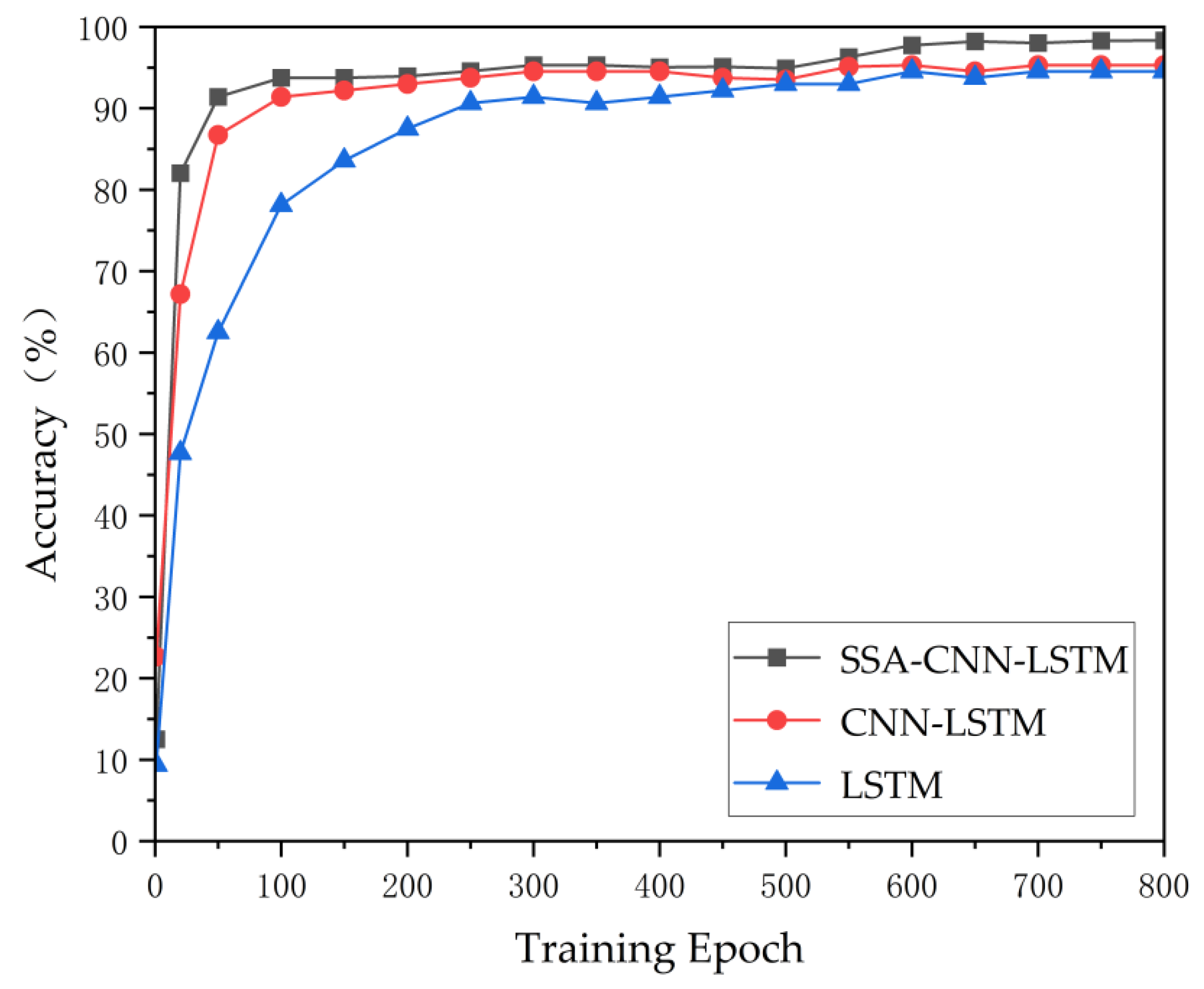
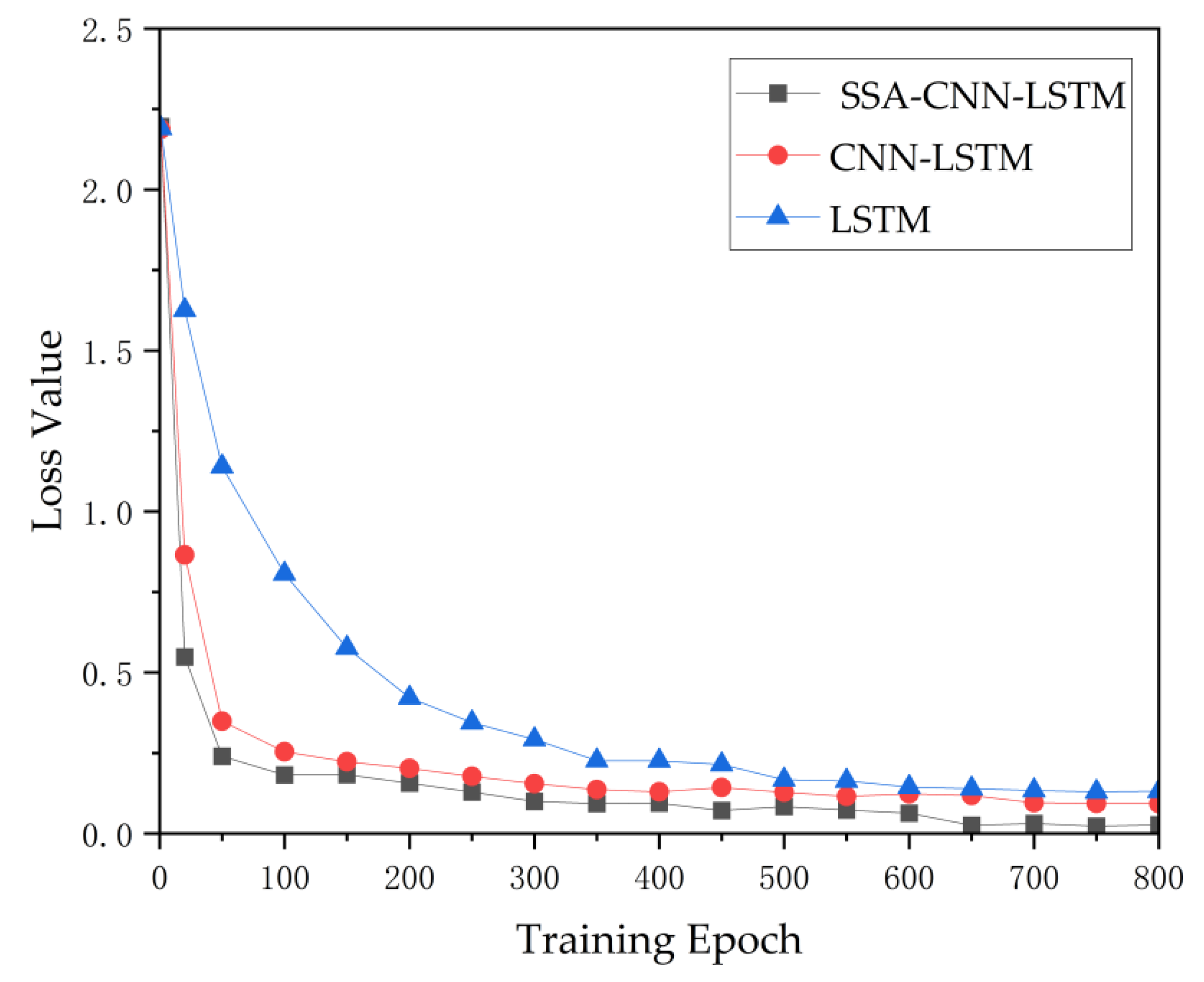
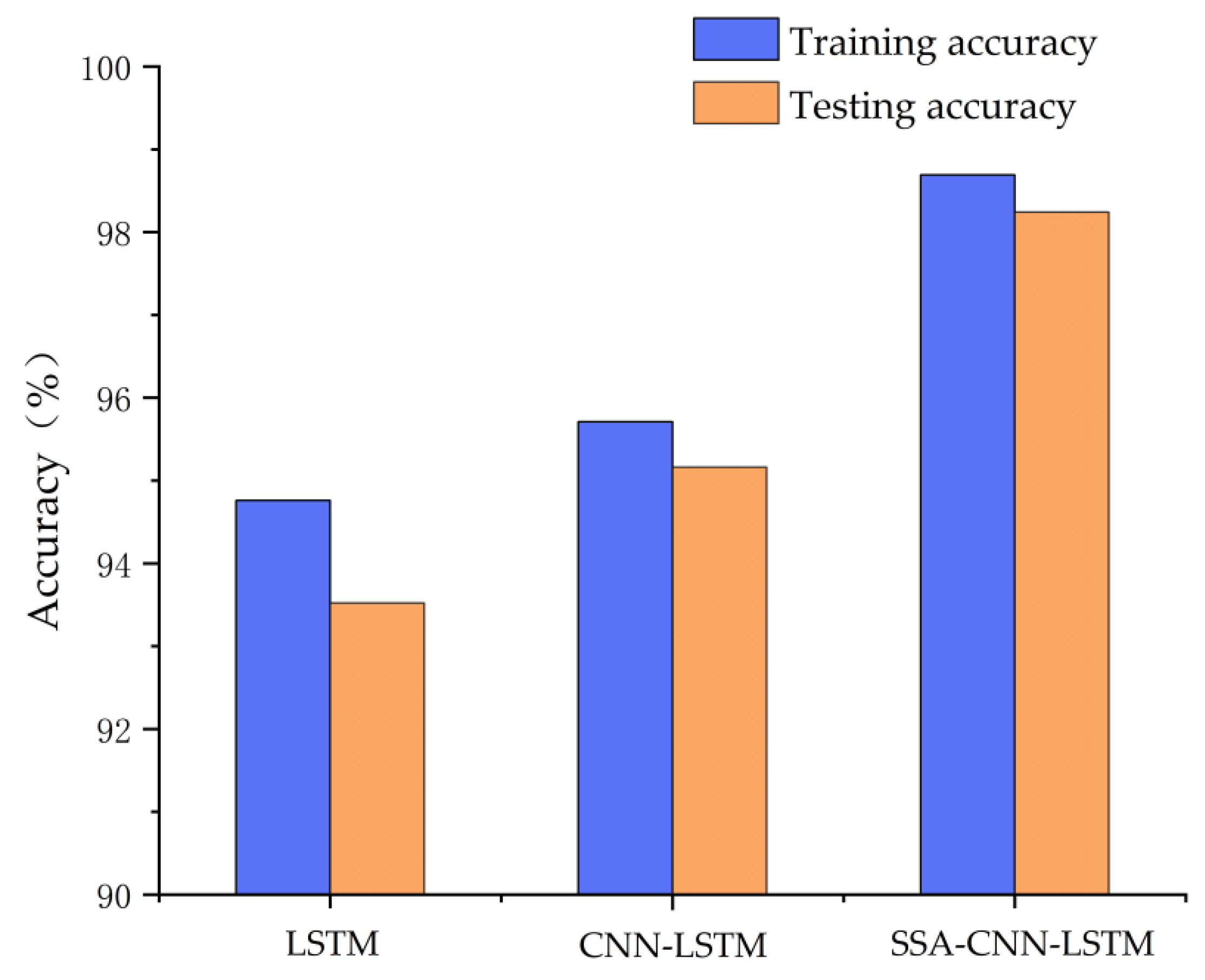
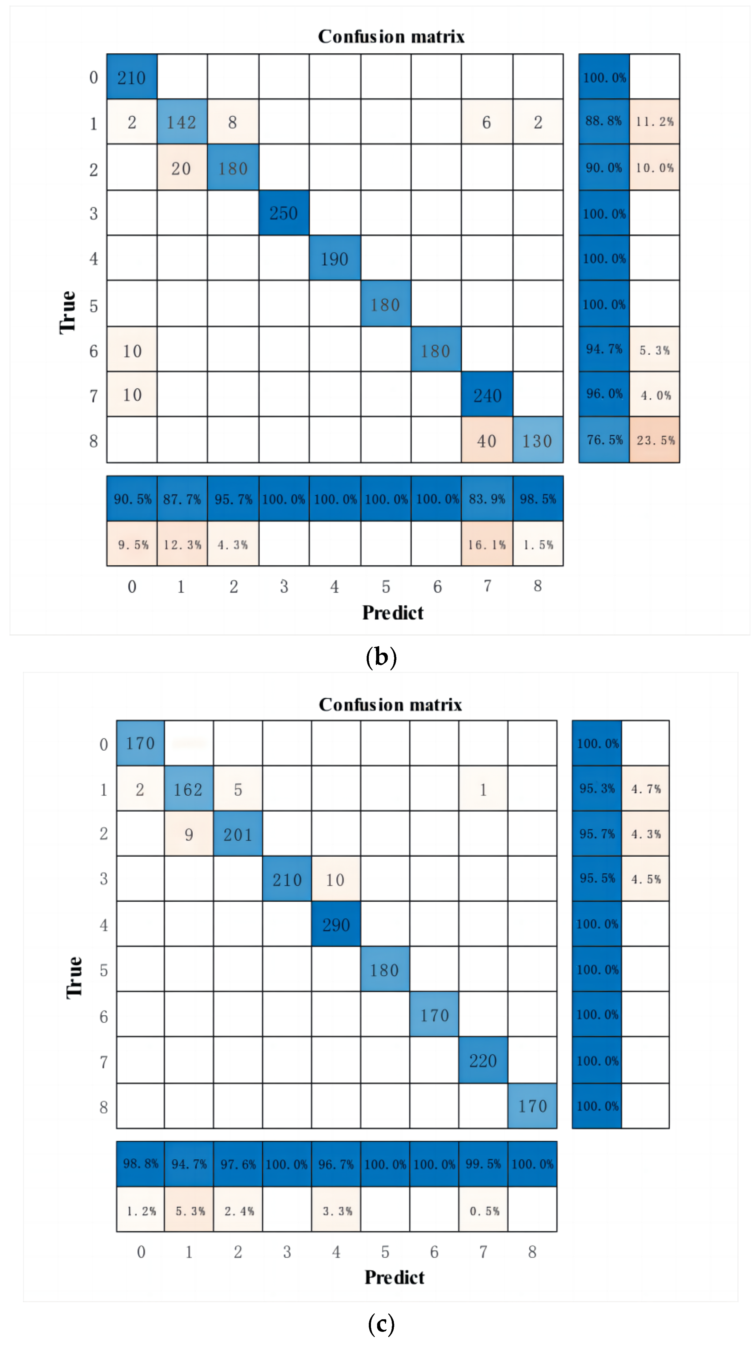
The SSA-CNN-LSTM model was validated using the run data of a PCTRAN and compared with the LSTM and CNN-LSTM models. The experimental results showed that the fault identification accuracy of the LSTM and CNN-LSTM models were 95.16% and 93.52%, respectively, and the fault identification accuracy of the SSA-CNN-LSTM model with the addition of the optimization algorithm was improved to 98.24%. All three models in the paper are capable of classifying nuclear power plant faults, but there will be differences in the accuracy of the classification. The SSA-CNN-LSTM model had the highest accuracy, which proves that the CNN-LSTM has a higher classification accuracy compared with a single model and that the SSA has a better effect on the optimization of the model.
Compared with the traditional machine learning model, the SSA-CNN-LSTM model proposed in this paper has the ability to process the complex data of nuclear power plants, can dig deeper into the timing characteristics, and has higher prediction accuracy in the fault diagnosis of nuclear power plants. When an accident occurs in a nuclear power plant, the SSA-CNN-LSTM model can determine the type of accident 0.22 s after the accident, which is of great significance for helping operators quickly identify faults, take corresponding measures in time, and improve the safety of nuclear power plant operation. However, this method has limitations. The accuracy of classification results will be reduced for unknown or untrained incidents. In the case of a small size in sample data, the model may not be able to fully learn the data features, and the accuracy may also be reduced. In addition, the training time of the SSA-CNN-LSTM model is long and is significantly longer than that of the LSTM neural network and CNN-LSTM model. Future research can improve models for these problems and further develop fault diagnosis models for nuclear power plants.


