

Zero-Phase FIR Filter Design Algorithm for Repetitive Controllers
 ,
,  , , , and
Abstract
:1. Introduction
2. Fundamentals of Repetitive Controllers
- must be a proper stable rational transfer function, in which ; and
- must hold.
2.1. Enlarging the Stability Domain of a Repetitive Control System
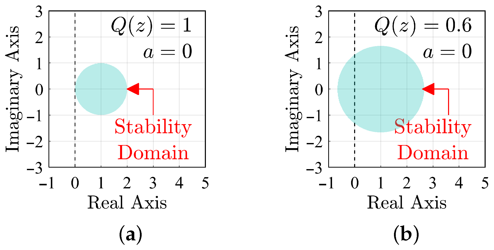
- as a constant attenuation: This solution promotes a constant reduction in the amplitude of the signal that is being fed back by the periodic signal generator of the repetitive controller, compromising its operation in relation to the internal model principle [20]. As a consequence, despite improving the system stability, it does not have a zero steady-state error. In order for the influence of to be small on the stationary error, it is usually chosen to be as close to one as possible. According to (6), the stability domain of the RC system is increased for (Figure 6). Examples of as a constant attenuation can be found in [10] (where ) and [11] (where ).
- as a FIR low-pass filter: This solution promotes the use of a low-pass filter in the periodic signal generator of the repetitive controller. Thus, it is expected that the dynamics of the control system will not be significantly altered for low frequencies, still making it possible to obtain a zero steady-state error (or as close to zero as possible). On the other hand, the repetitive controller will have a pass band defined by , thus, it will no longer control exogenous signals whose harmonic frequencies are beyond the cutoff frequency of the low-pass filter . The most common solution applied in the literature is (some examples are [24,25,26]).
2.2. Unified Approach to Evaluation of Repetitive Controllers
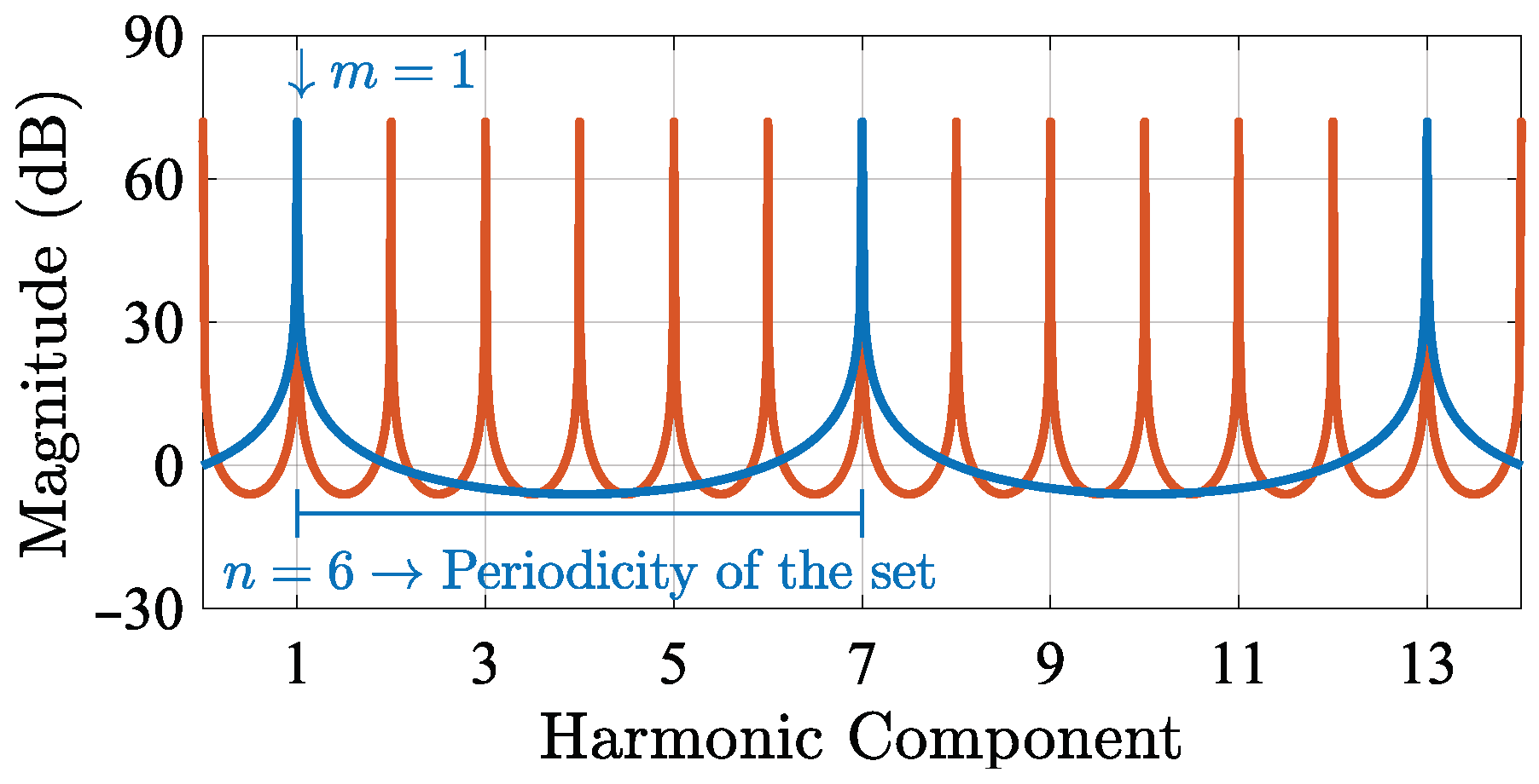
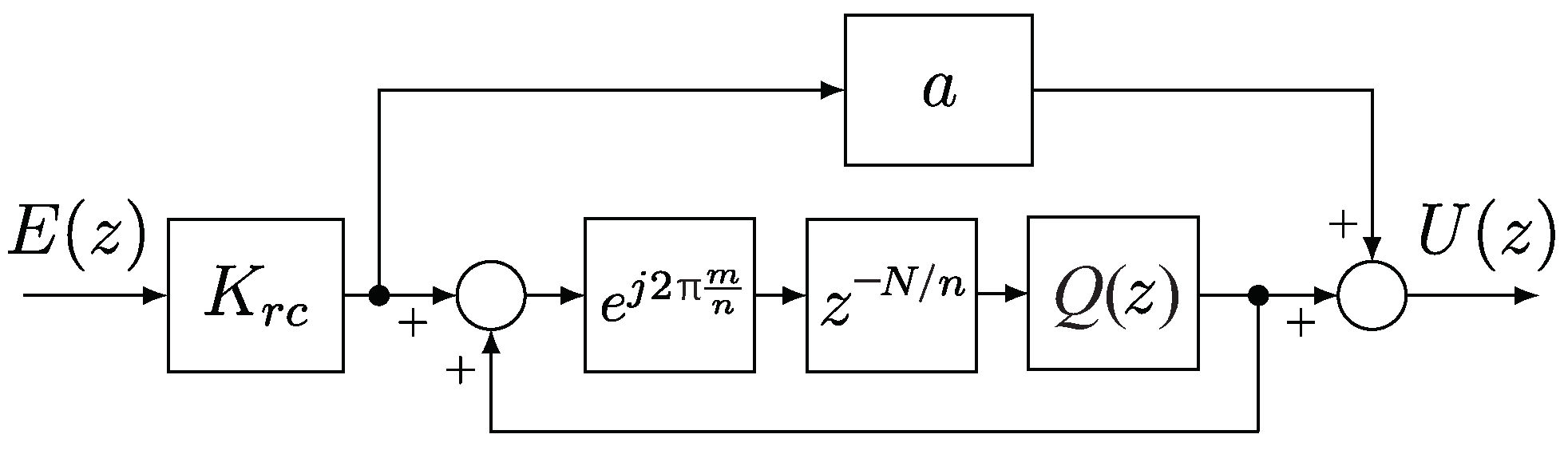
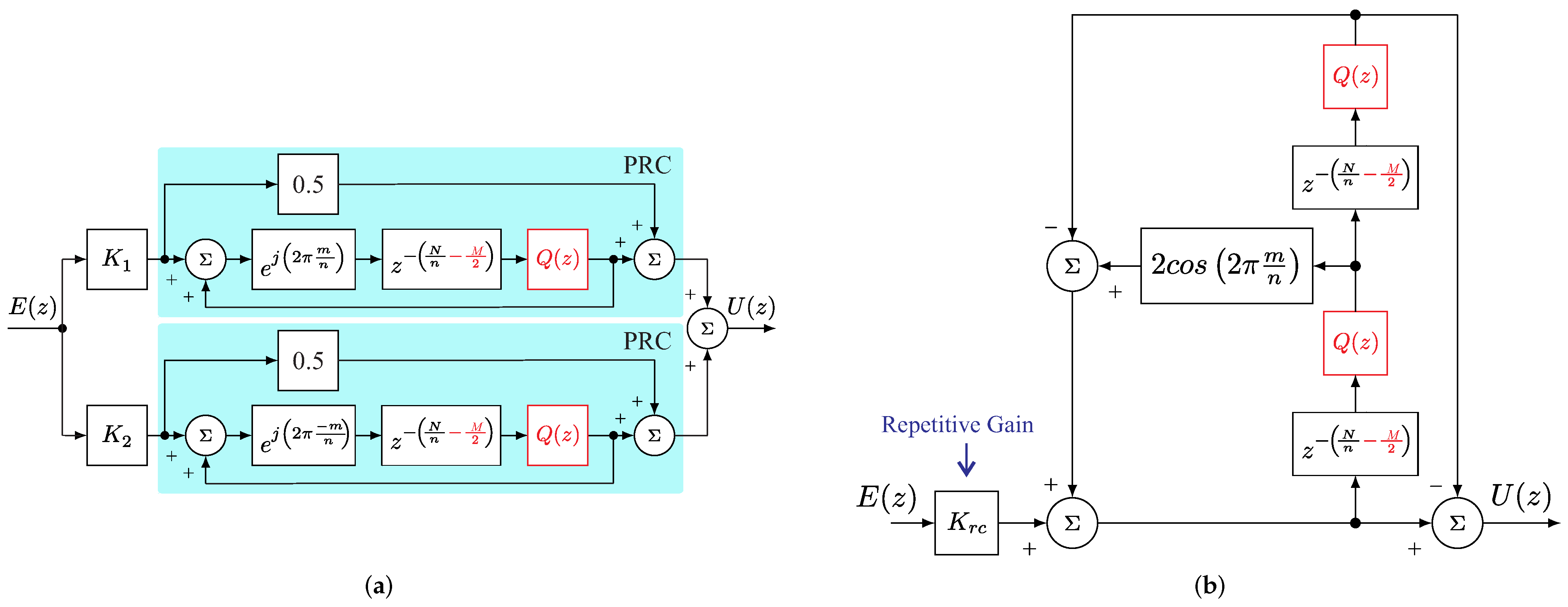
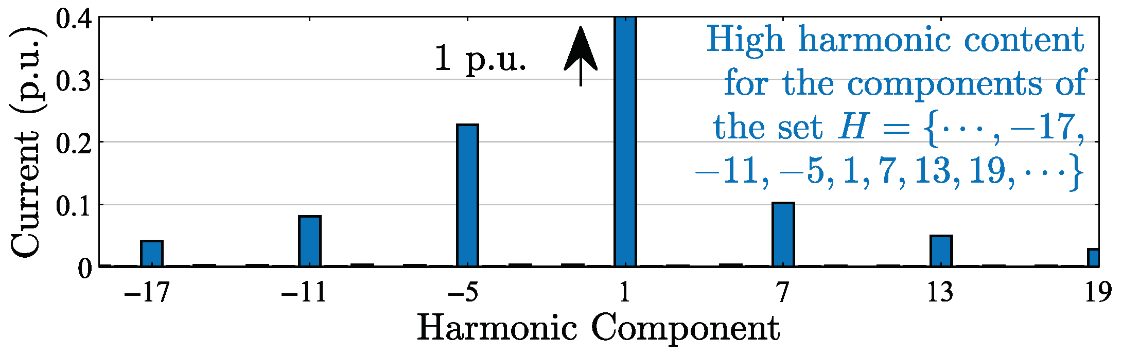
- A generic delay of samples (): The PRC has a generic delay of samples in its structure, in which N is the number of samples per fundamental period. The parameter n can be used to select the periodicity of the set of harmonic components that the PRC applies high gain (Figure 7). This means that, disregarding the other blocks presented below, the adequate selection of n allows the RC-based system to control periodic signals whose harmonics are in the set | instead of all harmonic components;
- A complex gain : If a complex gain is cascaded with the generic delay presented above, then the frequency response changes suffer frequency shifts. Therefore, the adequate selections of m and n allow for the RC-based system to control periodic signals whose harmonics are in the set | instead of |, where is restricted to .
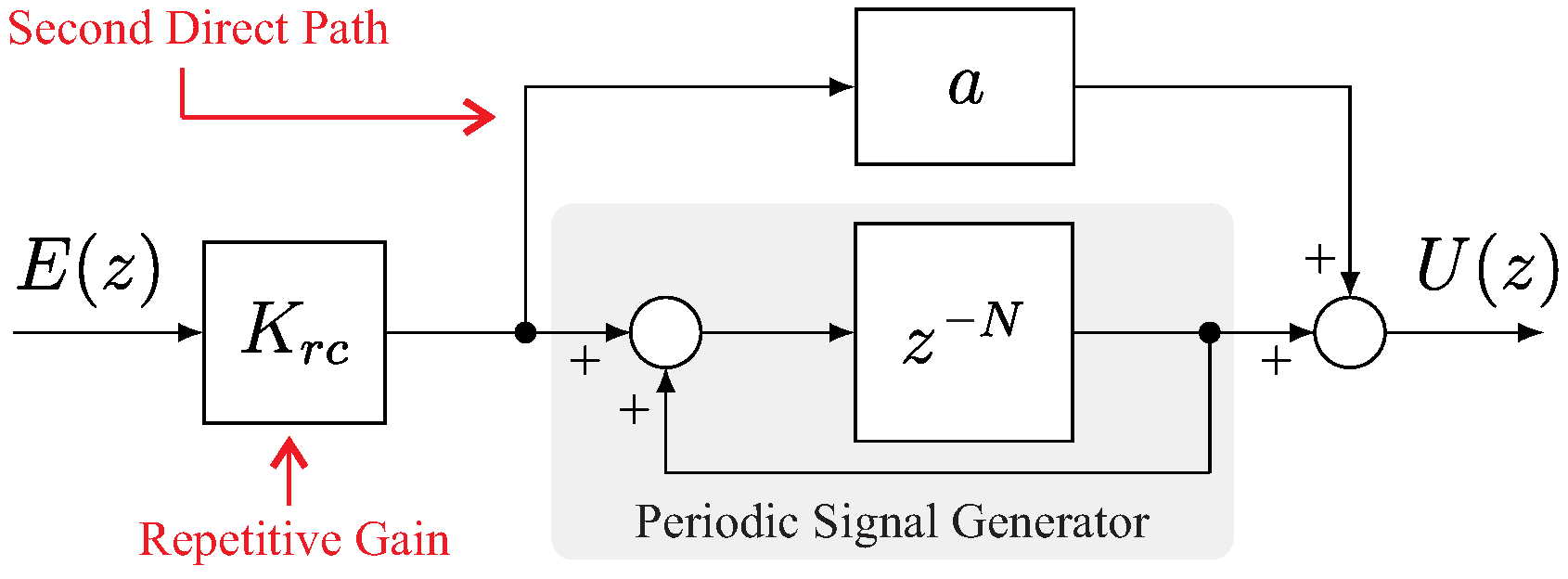
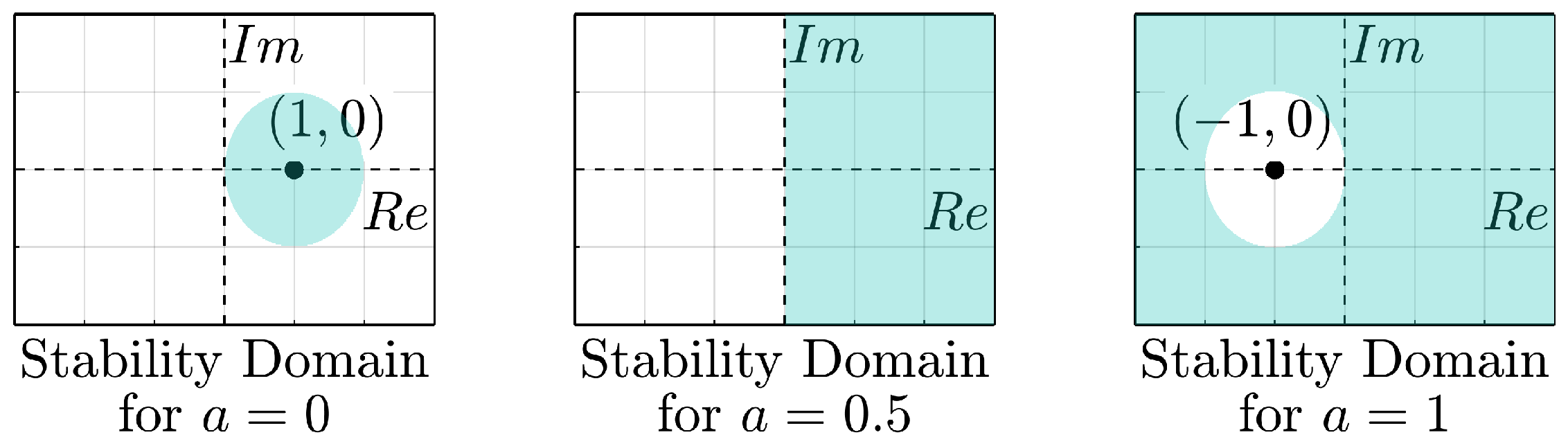
- A constant gain a: As done for the conventional repetitive controller [9], the PRC has a second direct path with the constant gain a. Gain a establishes a constant proportion between the repetitive action and a proportional action, and, as a consequence, it can be used to enlarge the stability domain of the control system [23]. Changes in this parameter do not make the stability domain contain the point (); thus, changes on this are not enough to make the repetitive controller applicable to strictly proper plants.
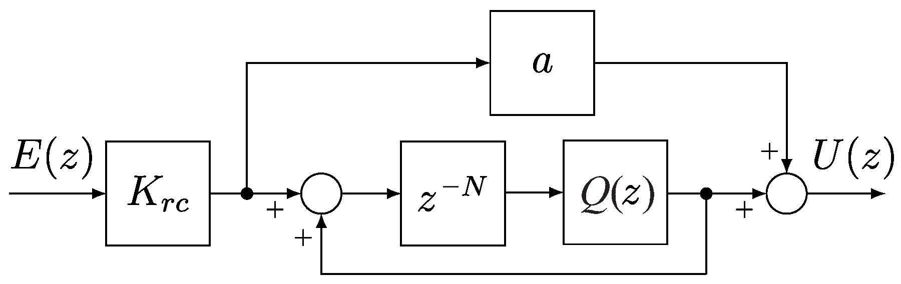
- A low-pass FIR filter : As described in Section 2.1, this block is usually a zero-phase FIR filter used to enlarge the stability domain of the control system.
3. Impact of the FIR Filter on the Stability and Performance of RC-Based Control Systems
- The frequency response of the controller will show a magnitude reduction for the frequency components beyond ), which means that the controller will reduce its ability to compensate for these frequency components (i.e., its bandwidth will be reduced);
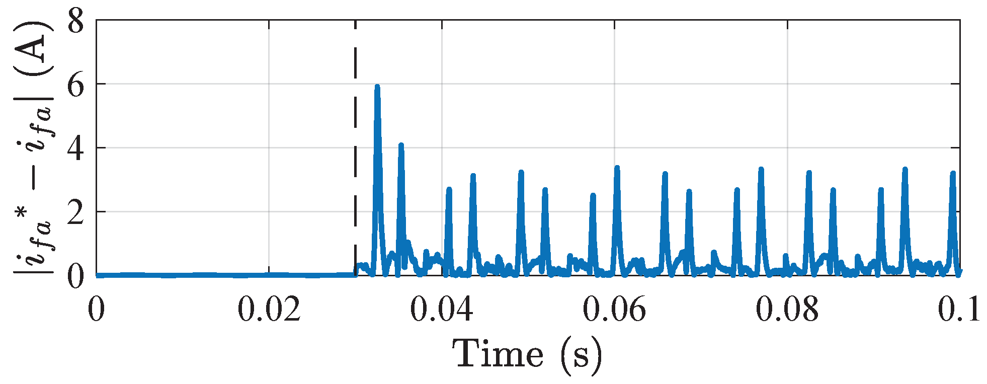
- Since FIR low-pass filters are not ideal, a small reduction in magnitude is expected for frequency components that are below but near the cutoff frequency . This reduction in magnitude means that the internal model principle [20] is not fully met, resulting in the controller not leading to zero steady-state error (Figure 11d). However, it is expected that the higher the , the lower the steady-state error should be.
4. Zero-Phase FIR Filter Design Algorithm
4.1. Obtaining the Specifications of a FIR Filter for a Repetitive Controller Using Its Stability Domain
- (a)
- STEP 1: Firstly, the control system designer must evaluate the exogenous signals of the control system and determine what are the harmonic components that must be controlled. Using this information, one can determine the passband of the repetitive controller. In this paper, it is considered that the RCs must work on exogenous signals with harmonic content up to .
- (b)
- STEP 2: Then, the control system designer must obtain the transfer function of the plant ( or ). According to [23], both continuous and discrete approaches leads to inequalities that result in the same stability domains, thus, any of them can be used.
- (c)
- STEP 3: As shown in Section 2, non-trivial RC-based controllers can be decomposed into PRCs in parallel (Figure 9). Thus, one must decompose the selected RC structure into PRCs in parallel, which can be done following the guidelines presented in [18]. Then, based on this decomposition, one must take note of parameter a obtained for these PRCs. This parameter remains constant during the execution of the algorithm and it will be used later to plot the stability domain of the RC system.
- (d)
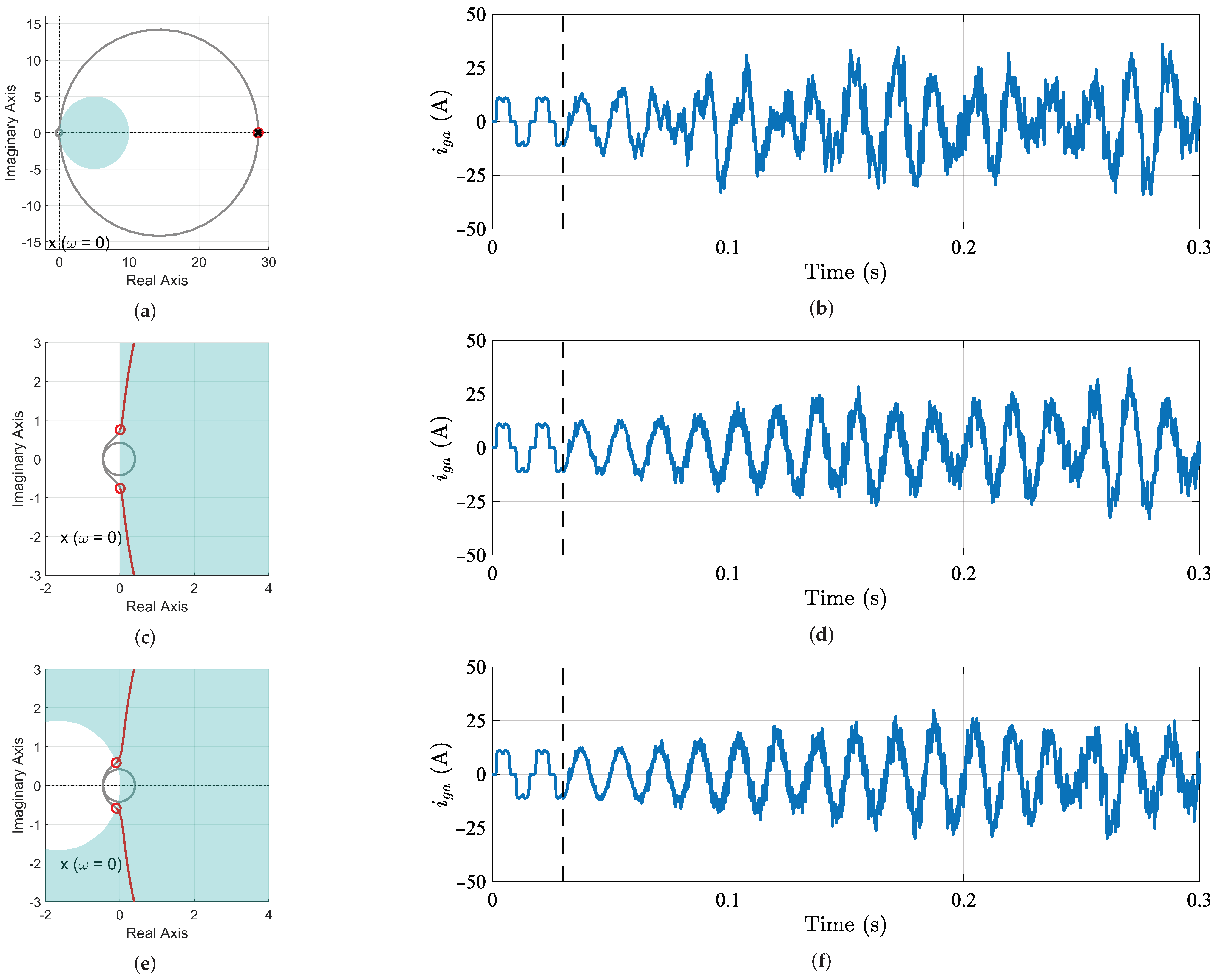
- STEP 4: and are initially set. Then, the Nyquist contour of (or ) together with the stability domain (which should be calculated for parameter a obtained in the previous step) must be plotted. Examples of this step are presented in Figure 12a,b.
- (e)
- STEP 5: As shown in Section 3, the bandwidth of the repetitive controller can be obtained by evaluating at which frequency the Nyquist contour of (or ) reaches the stability domain boundary. Thus, the repetitive gain can be tuned to select the highest frequency (here called as ) that, for , will be contained in the stability domain. Phase-margin and gain-margin can also be used to select the repetitive gain. Note that must be greater than . An example of this step is presented in Figure 12c;
- (f)
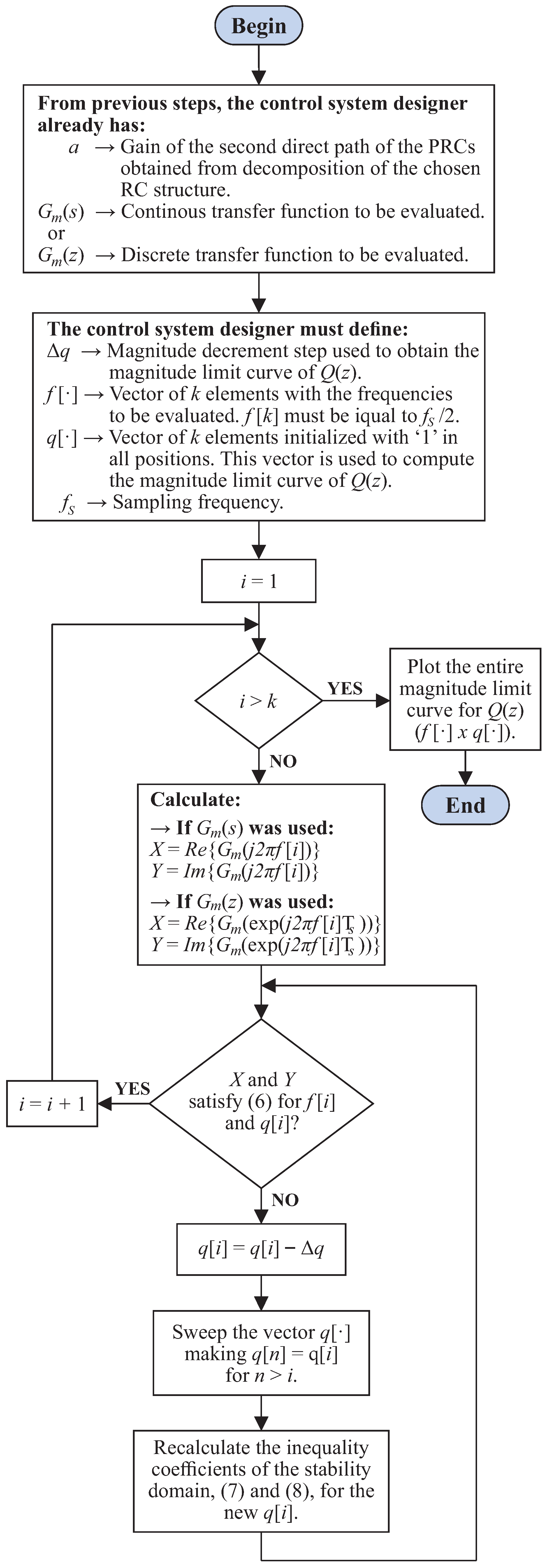
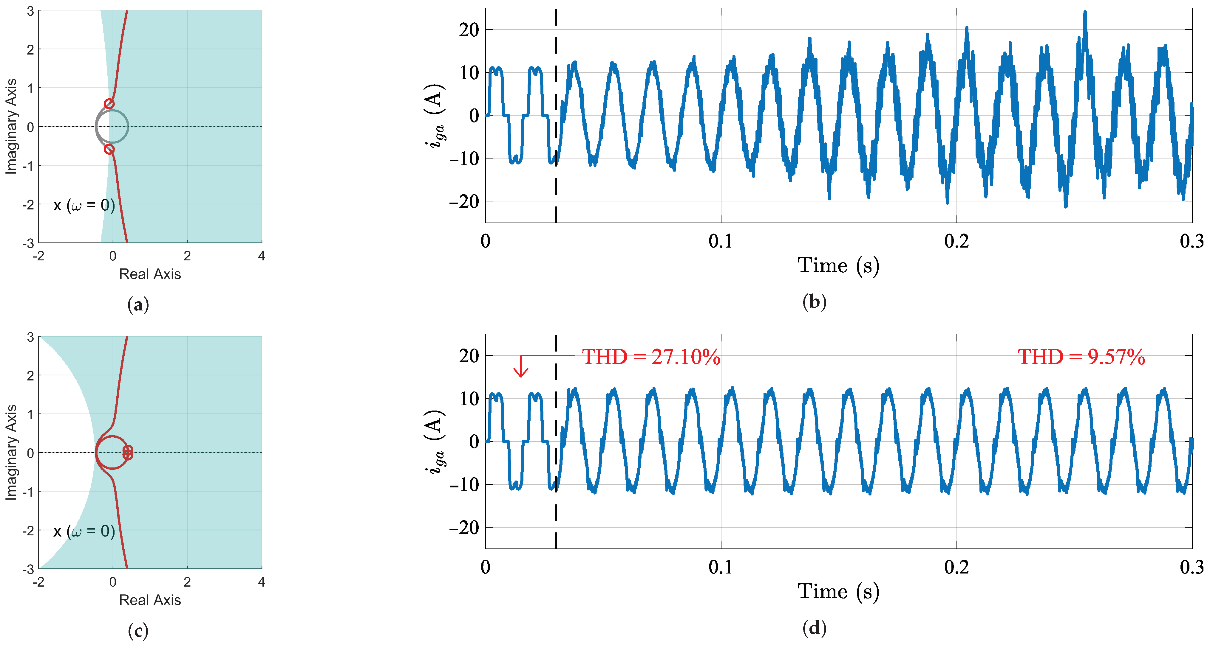
- STEP 6: As the magnitude of decreases, the maximum frequency of the Nyquist contour that is kept inside the stability domain increases (e.g., Figure 13). Based on this characteristic, the control system designer must gradually decrease the magnitude of in regular steps (here referred to as ), making it work as a constant attenuation (), while evaluates the highest frequency on the Nyquist contour of (or ) that still is inside the stability domain. By doing this, it becomes possible to determine the superior magnitude limit of for the entire frequency spectrum. An example of this step is shown in Figure 12d. This step is further detailed in the flowchart presented in Figure 14.
- (g)
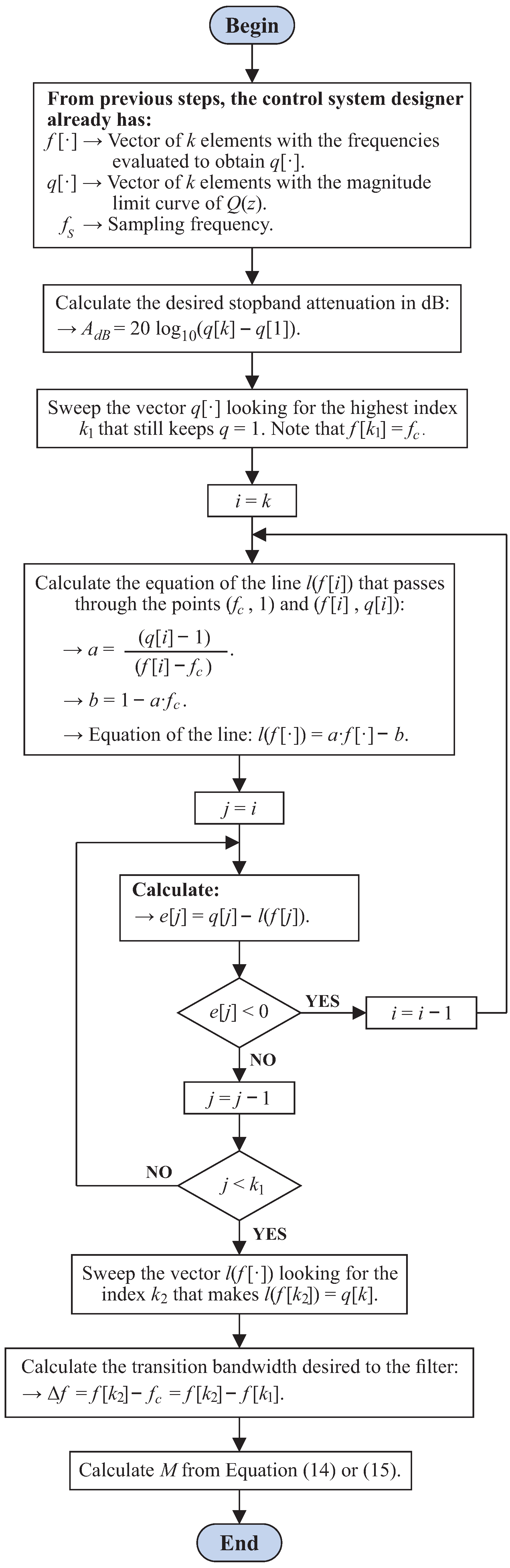
- STEP 7: With the curve plotted in STEP 6 (Figure 12d), one can estimate the order of the FIR filter (M) from the decay observed after the frequency . Firstly, one should calculate the line that tangents the decay (line in red in Figure 12e). From this line, one can obtain the parameters and (Figure 12e). Then, adapting from the Harris method [30], the order of the FIR filter can be estimated asin case is even, orin case results in an odd number. In (14) and (15), is the desired stop-band attenuation in dB; is the transition bandwidth desired to the filter; and is the sampling frequency. It must be noted that M must be even to maintain the FIR filter symmetry. As can be seen in (14) and (15), the filter order is increased by “+2” so that the decay slope is steeper around the filter cutoff frequency, making the system more robust and stable. This step is further detailed in the flowchart presented in Figure 15.
- (h)
- STEP 8: The specifications of the FIR filter are its order M and its cutoff frequency. In order to improve system performance, from this point on, the FIR filter cutoff frequency is considered as the frequency at which the superior magnitude limit curve of crosses dB (). The frequency is shown in Figure 12e. In case the superior magnitude limit curve does not cross dB, the frequency can be used as the cutoff frequency for the FIR filter. These data can be used to design the FIR filter using numeric computing software, such as Matlab. One can compare the magnitude response of the designed FIR filter with the curve plotted in STEP 6. An example of this comparison is presented in Figure 12f.
- (i)
- Firstly, is calculated from the difference between and . One must convert the subtraction result to a magnitude in dB.
- (ii)
- Then, one must obtain the equation of the line that passes through the points () and (). This equation is referred to here as .
- (iii)
- To obtain the line tangent to the decay of the magnitude limit curve of (line in red in Figure 12e), the flowchart calculates the error , with (where ). If the vector has any negative element, the line passes above the superior magnitude limit curve and, as a consequence, it is not yet the desired tangent line. Thus, the slope of the “tangent line” must be reduced, which can be done by changing the point () to () in the item and recalculating the line equation. This procedure is repeated until the vector has no negative elements.
- (iv)
- The parameter is calculated from the difference between and , where is equal to .
- (v)
- Finally, the parameter M can be calculated from and using (14).
4.2. Positioning the Zero-Phase FIR Filters in Non-Trivial RC-Based Controllers
5. Development of a Matlab app for Automatic Implementation of the Proposed Algorithm
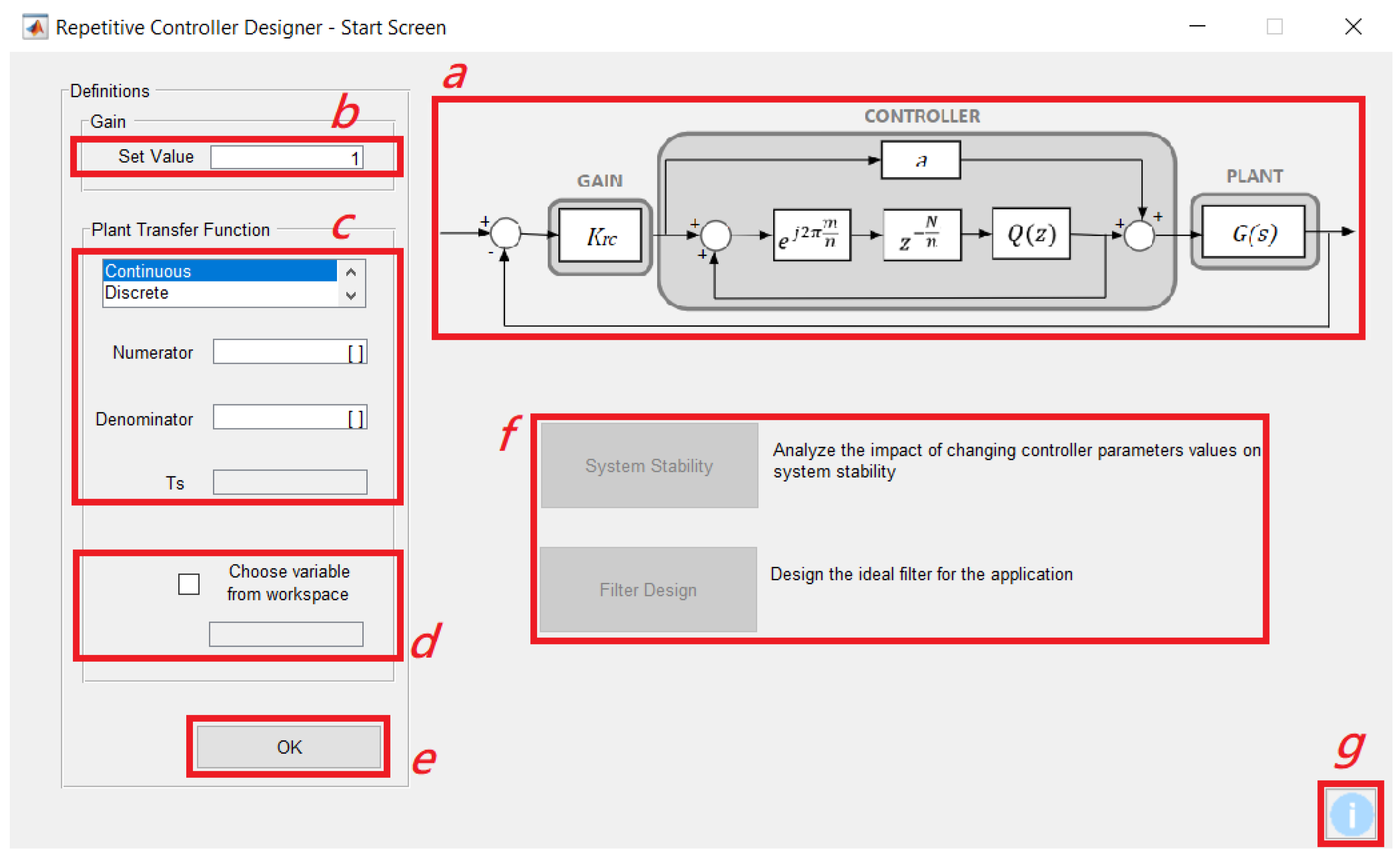
5.1. Start Screen
- It is verified if the repetitive gain is a real number of dimension 1 × 1;
- It is verified if the numerator and denominator fields are filled with row vectors; and
- When working with a discrete plant, it is verified if the sampling period is a real number of dimension 1 × 1.
- It is verified if the repetitive gain is a real number of dimension 1 × 1; and
- It is verified if the chosen variable exists and if it is one of the following types: tf (transfer function), zpk (zero-pole-gain), or ss (state space).
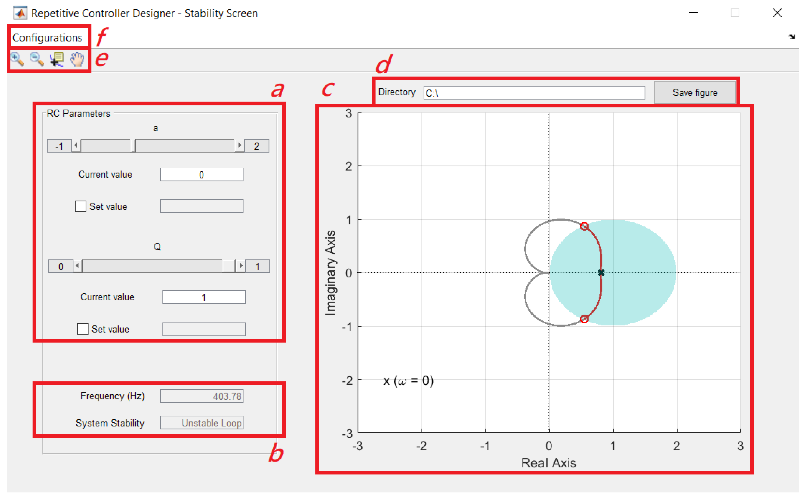
5.2. Stability Screen
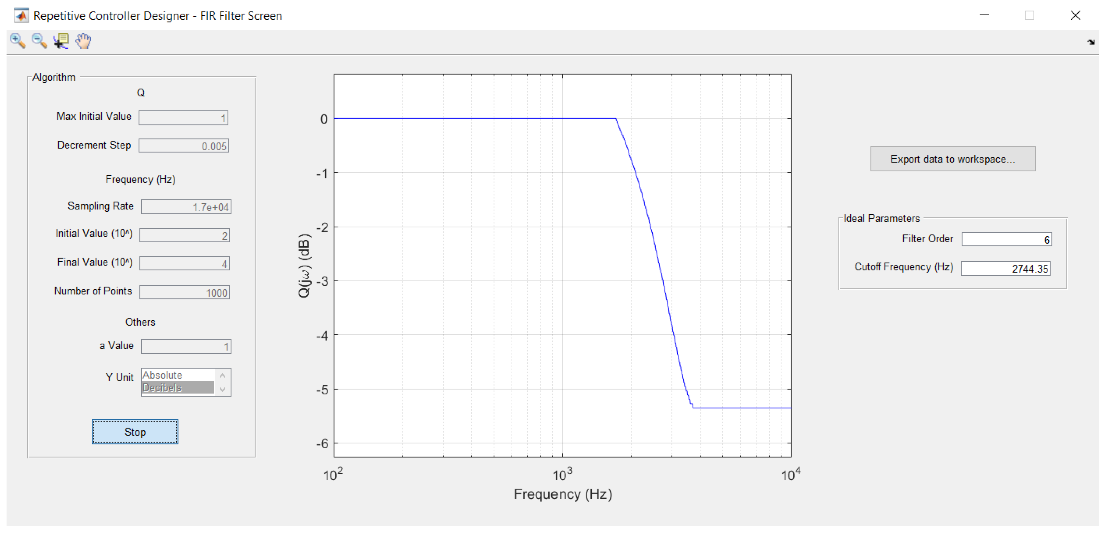
5.3. FIR Filter Screen
- The magnitude of for low frequencies, called the “max initial value” and the desired decrement for parameter . The authors recommend keeping the “max initial value” as one to make the Matlab app evaluate all possible values of );
- The initial and final values for the frequency evaluation and the number of frequencies to be evaluated between these extremes;
- Parameter a of the evaluated PRC;
- With respect to the graph that will be plotted, one must choose the Y-axis display mode, which can be “absolute” or “decibels” modes; and
- If the user defines the plant as continuous in the start screen, the sampling frequency of the discrete controller will also be required.
6. Experimental Validation
6.1. Description of the Experimental Setup
6.2. Description of the Evaluated Repetitive Control System
- (i)
- Firstly, the user would define a gain for the initial analysis in the start screen of the Matlab app;
- (ii)
- Then, the user would evaluate the stability of the system using parameter a and a constant attenuation—using the stability screen—or a FIR filter—using the FIR filter screen;
- (iii)
- Using the obtained parameters, the system must be simulated to verify whether the performance requirements are met or not;
- (iv)
- If the requirements are not met, the control system designer must increase or decrease the gain to make the system faster/slower and redo the process from step (ii).
6.3. Validation of the Matlab app and the Proposed Algorithms
6.3.1. System Stability Analysis Varying Only parameter a (With Being a Constant Attenuation)
6.3.2. System Stability Analysis Varying Parameters a and (With Being a Constant Attenuation)
6.3.3. Designing a FIR Filter for the RC System
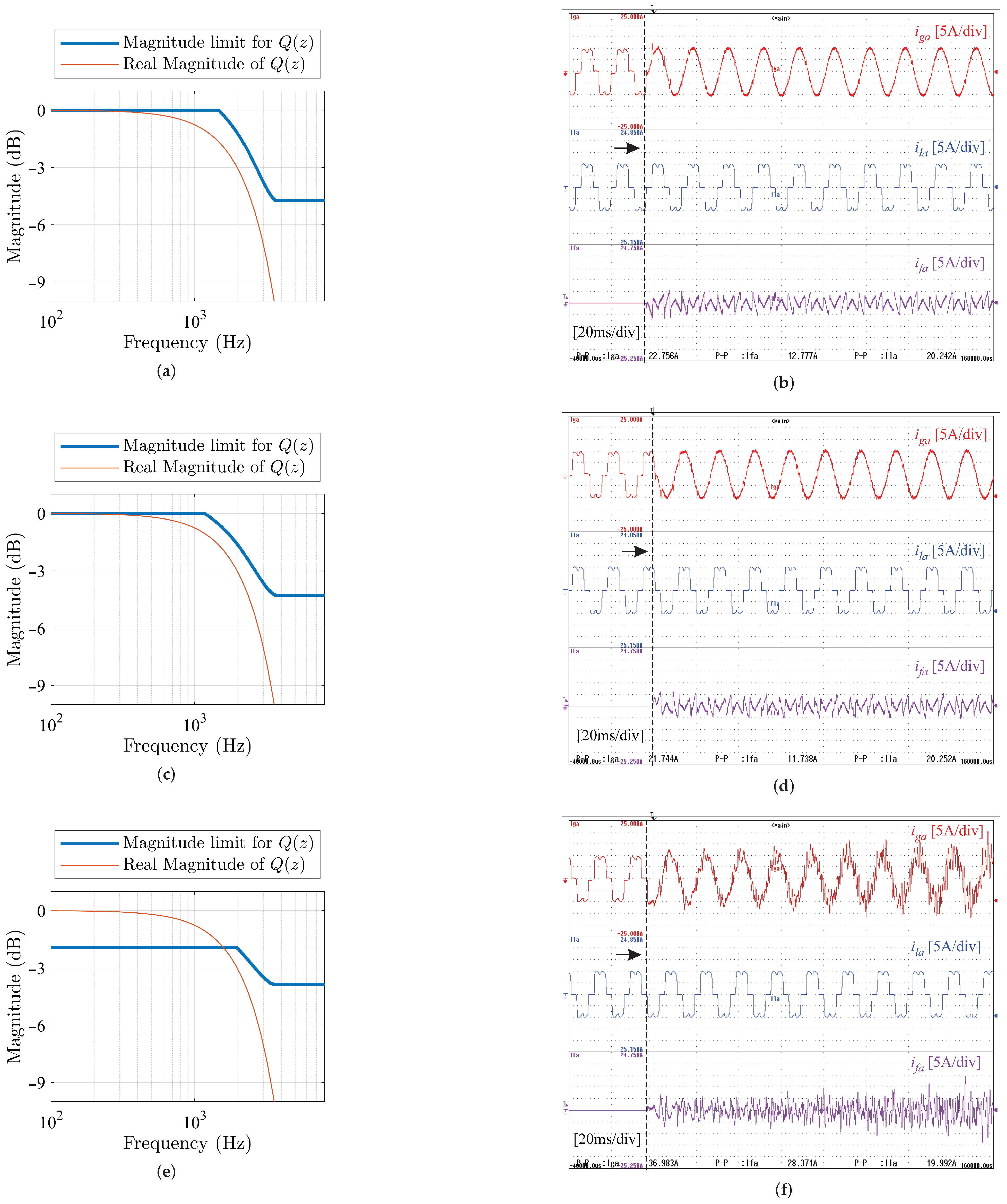
6.3.4. Error Analysis for Distinct Choices of Filter Characteristics
6.4. Performance Comparison
7. Conclusions
- The greater the passband of the FIR filter , the smaller the steady-state and transient errors of the RC system;
- Despite the characteristics mentioned in the previous item, the cutoff frequency of the FIR filter must not be high to the point of violating its superior magnitude limit. This limit can be obtained from the system stability analysis using the proposed Matlab app;
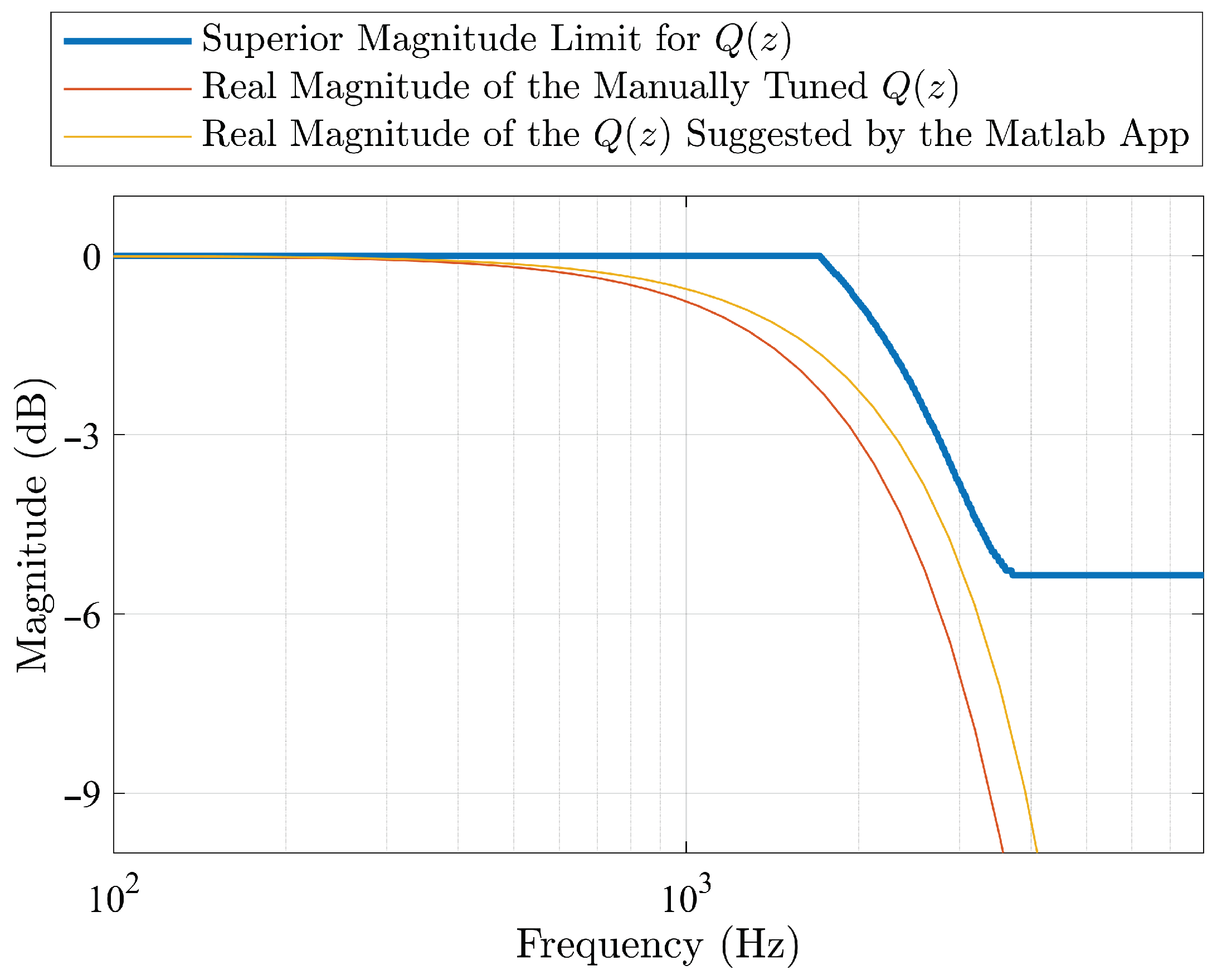
- The algorithm presented in this article is functional and it results in a FIR filter that does not violate its magnitude limits. Furthermore, the algorithm chooses a cutoff frequency for the filter that enables better steady-state results than most filters.
Author Contributions
Funding
Institutional Review Board Statement
Informed Consent Statement
Data Availability Statement
Conflicts of Interest
Abbreviations
| BIBO | Bounded-input, bounded-output |
| FIR | Finite impulse response |
| IIR | Infinite impulse response |
| ISE | Integral of the square of the error |
| ITAE | Integral of time multiplied by absolute error |
| PRC | Primitive repetitive cell |
| PWM | Pulse-width modulation |
| RC | Repetitive control |
| THD | Total harmonic distortion |
References
- Hu, C.; Yao, B.; Chen, Z.; Wang, Q. Adaptive Robust Repetitive Control of an Industrial Biaxial Precision Gantry for Contouring Tasks. IEEE Trans. Control. Syst. Technol. 2011, 19, 1559–1568. [Google Scholar] [CrossRef]
- Fateh, M.M.; Tehrani, H.A.; Karbassi, S.M. Repetitive control of electrically driven robot manipulators. Int. J. Syst. Sci. 2013, 44, 775–785. [Google Scholar] [CrossRef]
- Luo, Z.; Su, M.; Yang, J.; Sun, Y.; Hou, X.; Guerrero, J.M. A Repetitive Control Scheme Aimed at Compensating the 6k + 1 Harmonics for a Three-Phase Hybrid Active Filter. Energies 2016, 9, 787. [Google Scholar] [CrossRef] [Green Version]
- Neto, R.C.; De Souza, H.E.P.; Rech, C.; Neves, F.A. A nk pm m-Order Harmonic Repetitive Control Scheme with Improved Stability Characteristics. In Proceedings of the 2018 IEEE 27th International Symposium on Industrial Electronics (ISIE), Cairns, QLD, Australia, 13–15 June 2018; pp. 465–470. [Google Scholar]
- Biagiotti, L. Repetitive Control of Nonlinear Systems via Feedback Linearization: An Application to Robotics. In Proceedings of the 21st IFAC World Congress, Berlim, Germany, 11–17 July 2020; pp. 1468–1473. [Google Scholar]
- Liu, D.; Li, B.; Huang, S.; Liu, L.; Wang, H.; Huang, Y. An Improved Frequency-Adaptive Virtual Variable Sampling-Based Repetitive Control for an Active Power Filter. Energies 2022, 15, 7227. [Google Scholar] [CrossRef]
- Zhao, Q.; Zhang, H.; Gao, Y.; Chen, S.; Wang, Y. Novel Fractional-Order Repetitive Controller Based on Thiran IIR Filter for Grid-Connected Inverters. IEEE Access 2022, 10, 82015–82024. [Google Scholar] [CrossRef]
- Yuan, T.; Zhang, Y. Current Harmonic Suppression of BLDC Motor Utilizing Frequency Adaptive Repetitive Controller. Machines 2022, 10, 1071. [Google Scholar] [CrossRef]
- Hara, S.; Yamamoto, Y.; Omata, T.; Nakano, M. Repetitive control system: A new type servo system for periodic exogenous signals. IEEE Trans. Autom. Control 1988, 33, 659–668. [Google Scholar] [CrossRef] [Green Version]
- Lidozzi, A.; Ji, C.; Solero, L.; Zanchetta, P.; Crescimbini, F. Resonant–Repetitive Combined Control for Stand-Alone Power Supply Units. IEEE Trans. Ind. Appl. 2015, 51, 4653–4663. [Google Scholar] [CrossRef]
- Ji, C.; Zanchetta, P.; Carastro, F.; Clare, J. Repetitive Control for High-Performance Resonant Pulsed Power Supply in Radio Frequency Applications. IEEE Trans. Ind. Appl. 2014, 50, 2660–2670. [Google Scholar] [CrossRef]
- Oh, S.; Longman, R. Methods of Real-Time Zero-Phase Low-Pass Filtering for Robust Repetitive Control. In Proceedings of the AIAA/AAS Astrodynamics Specialist Conference and Exhibit, Monterey, CA, USA, 5–8 August 2002. [Google Scholar]
- Teo, Y.R.; Fleming, A.J. A new repetitive control scheme based on non-causal FIR filters. In Proceedings of the 2014 American Control Conference, Portland, OR, USA, 4–6 June 2014; pp. 991–996. [Google Scholar]
- Escobar, G.; Mattavelli, P.; Hernandez-Gomez, M.; Martinez-Rodriguez, P.R. Filters With Linear-Phase Properties for Repetitive Feedback. IEEE Trans. Ind. Electron. 2014, 61, 405–413. [Google Scholar] [CrossRef]
- Zhu, M.; Ye, Y.; Xiong, Y.; Zhao, Q. Parameter Robustness Improvement for Repetitive Control in Grid-Tied Inverters Using an IIR Filter. IEEE Trans. Power Electron. 2021, 36, 8454–8463. [Google Scholar] [CrossRef]
- Zimann, F.J.; Neto, R.C.; Neves, F.A.S.; de Souza, H.E.P.; Batschauer, A.L.; Rech, C. A Complex Repetitive Controller Based on the Generalized Delayed Signal Cancelation Method. IEEE Trans. Ind. Electron. 2019, 66, 2857–2867. [Google Scholar] [CrossRef]
- Panomruttanarug, B.; Longman, R.W. Frequency based optimal design of FIR zero-phase filters and compensators for robust repetitive control. Adv. Astronaut. Sci. 2006, 123, 219–238. [Google Scholar]
- Neto, R.C.; Neves, F.A.S.; De Souza, H.E.P. Unified Approach to Evaluation of Real and Complex Repetitive Controllers. IEEE Access 2021, 9, 47960–47975. [Google Scholar] [CrossRef]
- Inoue, T.; Nakano, M.; Kubo, T.; Matsumoto, S.; Baba, H. High Accuracy Control of a Proton Synchrotron Magnet Power Supply. In Proceedings of the 8th IFAC World Congress on Control Science and Technology for the Progress of Society, Kyoto, Japan, 24–28 August 1981; pp. 3137–3142. [Google Scholar]
- Francis, B.; Wonham, W. The internal model principle of control theory. Automatica 1976, 12, 457–465. [Google Scholar] [CrossRef]
- Mattavelli, P.; Marafao, F. Repetitive-based control for selective harmonic compensation in active power filters. IEEE Trans. Ind. Electron. 2004, 51, 1018–1024. [Google Scholar] [CrossRef]
- Neto, R.C.; Neves, F.A.S.; de Souza, H.E.P. Complex Controllers Applied to Space Vectors: A Survey on Characteristics and Advantages. J. Control Autom. Electr. Syst. 2020, 31, 1132–1152. [Google Scholar] [CrossRef]
- Neto, R.C.; Neves, F.A.S.; de Souza, H.E.P. Complex nk + m Repetitive Controller Applied to Space Vectors: Advantages and Stability Analysis. IEEE Trans. Power Electron. 2021, 36, 3573–3590. [Google Scholar] [CrossRef]
- Garcia-Cerrada, A.; Pinzon-Ardila, O.; Feliu-Batlle, V.; Roncero-Sanchez, P.; Garcia-Gonzalez, P. Application of a Repetitive Controller for a Three-Phase Active Power Filter. IEEE Trans. Power Electron. 2007, 22, 237–246. [Google Scholar] [CrossRef]
- Zhang, Y.; Dai, Z.; Fang, Y. Current Control of Shunt Active Power Filter Based on Repetitive Control. In Proceedings of the 2021 IEEE Sustainable Power and Energy Conference (iSPEC), Nanjing, China, 23–25 December 2021; pp. 2579–2584. [Google Scholar]
- Yang, Y.; Yang, Y.; He, L.; Fan, M.; Xiao, Y.; Chen, R.; Xie, M.; Zhang, X.; Zhang, L.; Rodriguez, J. A Novel Cascaded Repetitive Controller of an LC-Filtered H6 Voltage-Source Inverter. IEEE J. Emerg. Sel. Top. Power Electron. 2022, 61, 1516–1527. [Google Scholar] [CrossRef]
- Lu, W.; Zhou, K. A novel repetitive controller for nk ± m order harmonics compensation. In Proceedings of the 30th Chinese Control Conference, Yantai, China, 22–24 July 2011; pp. 2480–2484. [Google Scholar]
- Lu, W.; Zhou, K.; Wang, D.; Cheng, M. A Generic Digital nk ± m-Order Harmonic Repetitive Control Scheme for PWM Converters. IEEE Trans. Ind. Electron. 2014, 61, 1516–1527. [Google Scholar] [CrossRef]
- Lu, W.; Zhou, K.; Wang, D. General parallel structure digital repetitive control. Int. J. Control 2013, 86, 70–83. [Google Scholar] [CrossRef]
- Middlestead, R. Digital Communications with Emphasis on Data Modems: Theory, Analysis, Design, Simulation, Testing, and Applications; Wiley: Hoboken, NJ, USA, 2017. [Google Scholar]
- Neto, R.C.; Neves, F.A.S.; de Souza, H.E.P.; Zimann, F.J.; Batschauer, A.L. Design of Repetitive Controllers Through Sensitivity Function. In Proceedings of the 2018 IEEE 27th International Symposium on Industrial Electronics (ISIE), Cairns, Australia, 13–15 June 2018; pp. 495–501. [Google Scholar]
- MathWorks. Packaging and Installing MATLAB Apps. Available online: https://www.mathworks.com/videos/packaging-and-installing-matlab-apps-101563.html (accessed on 30 December 2022).
- MathWorks. MATLAB App Installer File—mlappinstall. Available online: https://www.mathworks.com/help/matlab/creating_guis/what-is-an-app.html (accessed on 30 December 2022).
- Limongi, L.R.; Bojoi, R.; Griva, G.; Tenconi, A. Digital current-control schemes. IEEE Ind. Electron. Mag. 2009, 3, 20–31. [Google Scholar] [CrossRef] [Green Version]
- Tang, Y.; Loh, P.C.; Wang, P.; Choo, F.H.; Gao, F.; Blaabjerg, F. Generalized Design of High Performance Shunt Active Power Filter With Output LCL Filter. IEEE Trans. Ind. Electron. 2012, 59, 1443–1452. [Google Scholar] [CrossRef]
- Neto, R.C.; Neves, F.A.S.; Stangler, E.V.; Bradaschia, F.; de Souza, H.E.P. Structural and Performance Comparison Between Harmonic Selective Repetitive Controllers for Shunt Active Power Filter. In Proceedings of the 2019 IEEE 15th Brazilian Power Electronics Conference and 5th IEEE Southern Power Electronics Conference (COBEP/SPEC), Santos, Brazil, 1–4 December 2019; pp. 1–8. [Google Scholar]
- Neto, R.C.; Neves, F.A.S.; Azevedo, G.M.S.; de Souza, H.E. A Comparison Between Real and Complex Harmonic Selective Repetitive Control Schemes with Improved Stability Characteristics. In Proceedings of the IECON 2019—45th Annual Conference of the IEEE Industrial Electronics Society, Lisbon, Portugal, 14–17 October 2019; Volume 1, pp. 7019–7025. [Google Scholar]
- Buso, S.; Mattavelli, P. Digital Control in Power Electronics; Lectures on Power Electronics; Morgan & Claypool Publishers: San Rafael, CA, USA, 2006. [Google Scholar]
- IEEE Std 519-2014 (Revision of IEEE Std 519-1992); IEEE Recommended Practice and Requirements for Harmonic Control in Electric Power Systems. IEEE: New York, NY, USA, 2014; pp. 1–29.


| Parameters of the Repetitive Controller | Parameters of the Experimental Setup (Figure 21) | |||||||||||
|---|---|---|---|---|---|---|---|---|---|---|---|---|
| n | m | * | ||||||||||
| 6 | 1 | 288 | 380 V | H | m | mH | mH | m | 600 V | kHz | 60 Hz | |
| Parameters | |
|---|---|
| Parameter a | 1 |
| Maximum initial value | 1 |
| Decrement step () | |
| Sampling rate | kHz |
| Initial frequency | 100 Hz |
| Final frequency | 10 kHz |
| Number of evaluated frequencies | 1000 |
| Results | |
| Filter Order (M) | 6 |
| dB Cutoff Frequency () | kHz |
| Cases | Evaluated Scenarios | THD | ISE () | ITAE () |
|---|---|---|---|---|
| Grid currents without SAPF | – | – | ||
| SAPF controlled by a RC with as a constant attenuation (). | ||||
| SAPF controlled by a RC with FIR filter presented in Section 6.3.3 ( and kHz) | ||||
| SAPF controlled by a RC with FIR filter suggested by the Matlab app ( and kHz) |
Disclaimer/Publisher’s Note: The statements, opinions and data contained in all publications are solely those of the individual author(s) and contributor(s) and not of MDPI and/or the editor(s). MDPI and/or the editor(s) disclaim responsibility for any injury to people or property resulting from any ideas, methods, instructions or products referred to in the content. |
© 2023 by the authors. Licensee MDPI, Basel, Switzerland. This article is an open access article distributed under the terms and conditions of the Creative Commons Attribution (CC BY) license (https://creativecommons.org/licenses/by/4.0/).
Share and Cite
de Lima, P.V.S.G.; Neto, R.C.; Neves, F.A.S.; Bradaschia, F.; de Souza, H.E.P.; Barbosa, E.J. Zero-Phase FIR Filter Design Algorithm for Repetitive Controllers. Energies 2023, 16, 2451. https://doi.org/10.3390/en16052451
de Lima PVSG, Neto RC, Neves FAS, Bradaschia F, de Souza HEP, Barbosa EJ. Zero-Phase FIR Filter Design Algorithm for Repetitive Controllers. Energies. 2023; 16(5):2451. https://doi.org/10.3390/en16052451
Chicago/Turabian Stylede Lima, Pedro V. S. G., Rafael C. Neto, Francisco A. S. Neves, Fabrício Bradaschia, Helber E. P. de Souza, and Eduardo J. Barbosa. 2023. "Zero-Phase FIR Filter Design Algorithm for Repetitive Controllers" Energies 16, no. 5: 2451. https://doi.org/10.3390/en16052451