An FCS-MPC Strategy for Series APF Based on Deadbeat Direct Compensation

Abstract

Aiming at the delay caused by the phase-locked loop (PLL) and harmonic detection in the traditional control of a series active power filter (SAPF), a deadbeat direct control (DBDC)-based finite control set model predictive control (FCS-MPC) strategy for the SAPF is proposed in this work. Firstly, a reference voltage generation mechanism based on direct control is established, which avoids the delay in harmonic detection, thus improving the dynamic response performance of the system. Secondly, the reference current generation mechanism suitable for the SAPF is derived and established using the deadbeat control (DBC) in the αβ coordinate system, based on which the FCS-MPC system is constructed. It eliminates the complex coordinate transformation and PLL and effectively compensates for the full-frequency harmonic voltage. Finally, the proposed control strategy is verified by a simulation and an experiment. The results suggest that the proposed control strategy can effectively compensate for the load voltage and suppress harmonic distortion for the temporary swell and sag of the grid voltage, sudden load changes, and harmonic distortion conditions.

1. Introduction

Owing to the rapid development and wide application of distributed power supply, distributed energy storage, new power electronic load, and other devices in the power system, the power electronic characteristics of the system are increasingly apparent [1,2]. It increases the harmonics and distortion rate and affects the quality of power supply. In addition, the fluctuation and intermittent characteristics of new energy power generation will aggravate power quality such as voltage fluctuation and flickering [3,4]. As a type of power electronic equipment, the series active power filter (SAPF) is used for dynamic voltage compensation and harmonic suppression, which can quickly track and solve the voltage quality problems caused by shock load and nonlinear load [5,6].

At present, commonly used control strategies in the active power filter (APF) include hysteresis control [7,8], double closed-loop proportional–integral (PI) control [9,10,11], and repetitive control [12,13]. Hysteresis control is easy to implement but exhibits a compensation performance easily affected by the hysteresis width and a large fluctuation in switching frequency. A virtual sampling and switching time prediction method was designed based on the variable hysteresis width strategy in [14], which solved the switching frequency fluctuation near the zero crossing of the power grid voltage, but its control accuracy could not be guaranteed. PI control shows good dynamic performance and a wide application range. It could realize no-static error tracking for direct current (DC) signals but was disadvantaged with steady-state error and phase delay for alternative current (AC) voltage signals containing harmonics. Therefore, quasi-proportional resonant (QPR) control is generally selected to track and control the specified frequency harmonics. For multiple harmonic compensations, however, the multiple QPR controllers should be arranged in parallel, which exhibits a complex control structure [15,16]. Repetitive control is realized by integrating periodic signals to realize non-static error tracking, with high control accuracy and good suppression in a periodic disturbance. However, it fails to satisfy the performance requirements of SAPF dynamic control due to a long delay. In [17], a double closed-loop control system, taking repetitive control and PI as the outer and inner loops, respectively, is proposed to improve the dynamic performance of a three-phase four-bridge arm APF. However, its application is restricted due to the inherent defects of repetitive control. Additionally, in order to eliminate the influence of current harmonics in an APF with a multilevel inverter, [18,19,20] researched and improved modulation techniques to effectively reduce system calculations and harmonic distortion rates but did not mention the suppression of voltage harmonics.

Predictive control has attracted much attention in power electronic converter control recently, including the model predictive control (MPC) strategy and the deadbeat control (DBC) strategy [21]. Finite control set model predictive control (FCS-MPC) is advantaged with a simple control structure and no pulse-width modulation (PWM) link, and it has become one of the main research directions at present [22,23,24]. Currently, there are few research studies on the FCS-MPC strategy of the SAPF, most of which focus on the parallel active power filter (PAPF). For cascaded PAPFs, a multi-step FCS-MPC cost function simplification method is proposed in [25], which obtains the harmonic reference signal based on the three-level redundant switching characteristics, balances the capacitor voltage on the DC side, and makes the target optimization caused by weight factor selection easier. As described in [26], the dynamic reactive power compensated for a hybrid APF (HAPF). Meanwhile, multi-variable FCS-MPC and an adaptive notch filter are employed to suppress the resonance and improve the dynamic response of the HAPF. [27] applied FCS-MPC to an inductor–capacitor–inductor (LCL)-type grid-connected inverter. After the state feedback method was optimized, the switching loss of inverters was reduced, and the quality of the grid-connected current was improved, which reveals the huge application potential of FCS-MPC. High dynamic performance and easy implementation make the FCS-MPC for the SAPF strategy worthy of further exploration.

With a differential prediction model, DBC can take the measured value and reference value of the state variable as the initial value and the actual value, respectively, ideally making the state variable track the instruction in the subsequent control cycle [28,29]. For a single-phase PAPF, [30] proposed a reference current generation mechanism and digital DBC current controller to ensure the stability of the current control system under uncertain parameters. Meanwhile, a DBC current controller suitable for an LC-coupling HAPF is designed in [31], which can accurately track the reference compensation current, exhibits a small steady-state error and a fast dynamic response, and can maintain a fixed switching frequency with a small output current ripple. However, the reference signals should be modulated, and the control system structure is complex.

Most current studies on SAPF control select indirect control, which inevitably leads to system delay caused by the PLL and harmonic detection. Hence, a DBDC-FCS-MPC strategy for the SAPF is proposed in this work. The main contributions are as follows.

Firstly, the voltage reference signal is generated directly between the ideal load voltage and the actual grid voltage based on direct control, which eliminates the PLL and detection link, avoiding the delay of the harmonic detection. Secondly, based on the DBC principle, the SAPF mathematical model of the αβ coordinate system is deduced, and the reference current generation mechanism is established, which eliminates the complicated coordinate transformation and cross coupling in voltage outer loop control. In addition, the dynamic performance of the system is further improved, and the full-frequency harmonic voltage is compensated. Finally, a DBDC-FCS-MPC strategy for the SAPF is constructed to realize voltage compensation control without harmonic detection, a PLL, a closed-loop controller, and PWM.

The structure of this work is as follows. The basic working principle of the SAPF and the mathematical modeling of the system are elaborated in Section 2. The DBDC-FCS-MPC strategy for the SAPF is detailed in Section 3. In Section 4, the proposed control strategy is analyzed and verified by a simulation and an experiment. Finally, this work is summarized in Section 5.

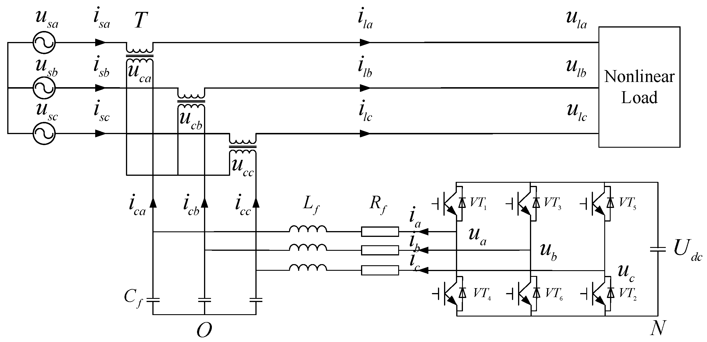
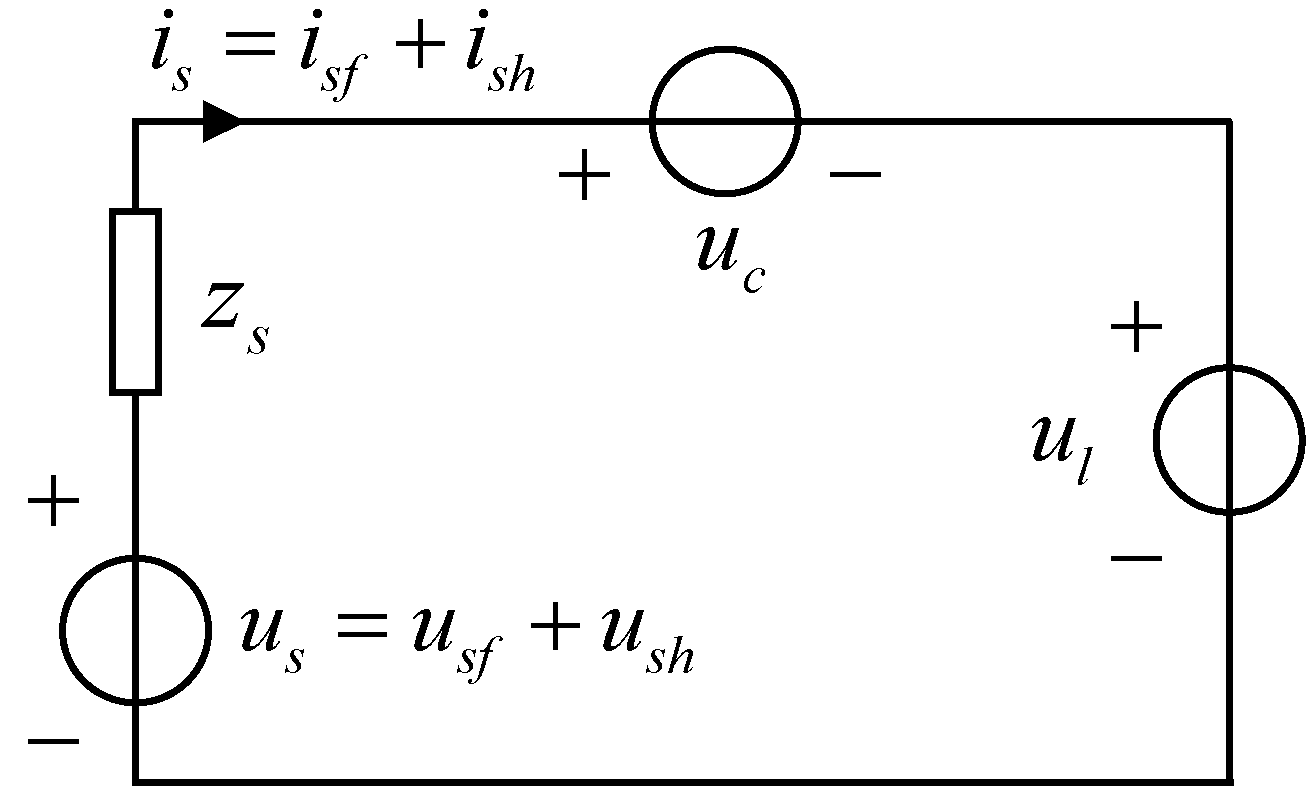
2. The System Structure and Mathematical Model of SAPF

The topology structure of the three-phase two-level SAPF system is illustrated in Figure 1. The three-phase power grid is connected to the nonlinear load and the SAPF through a series transformer. In the figure $u_{sa}$, $u_{sb}$, and $u_{sc}$ refer to the voltages of the three-phase grid, and $i_{sa}$, $i_{sb}$, and $i_{sc}$ represent the currents; $u_{la}$, $u_{lb}$, and $u_{lc}$ stand for voltages of the three-phase load voltages, and $i_{la}$, $i_{lb}$, and $i_{lc}$ represent load currents; $u_{ca}$, $u_{cb}$, and $u_{cc}$ represent the three-phase output voltages of the SAPF, and $i_{ca}$, $i_{cb}$, and $i_{cc}$ are the output currents; $u_a$, $u_b$, and $u_c$ represent the three-phase output voltages of the inverter, and $i_a$, $i_b$, and $i_c$ are output currents. The main circuit is the voltage source inverter. Meanwhile, VT1-VT6 are the six fully controlled power semiconductor devices (insulated gate bipolar translators (IGBTs)) of the three-phase bridge arms. $U_{dc}$ represents the voltage on the DC side and is responsible for the energy supply of the main circuit, and N is the ground point on the DC side. In addition, L_f and R_f represent filter inductance and parasitic resistance on the inverter side, respectively. C_f refers to filter capacitance, and O is the neutral point of the three-phase power grid and is selected as the zero-potential reference point. The primary and secondary windings of the transformer T are connected using the “Y, d” mode, and the winding ratio is changed. In this work, the three-phase uncontrolled rectifier bridge with resistive load is taken as the nonlinear load.

Figure 2 shows the single-phase equivalent circuit when the SAPF compensates for the harmonic voltage, where $z_s$ is the equivalent impedance of the system; $u_c$ represents the compensation voltage emitted by the SAPF; and $u_l$ refers to the load voltage. In addition, the grid voltage $u_s$ and current $i_s$ consist of the fundamental components $u_{sf}$ and $i_{sf}$ and the harmonic components $u_{sh}$ and $i_{sh}$, respectively.

During the operating, the SAPF behaves as a high impedance to harmonics of magnitude equal to k, as follows:

$$i_{sh}=\frac{u_{sh}}{z_s+k}$$

(1)

At this time, the SAPF is equivalent to the harmonic isolator between the grid and the load. When k tends to infinity, the harmonic current of the grid satisfies $i_{sh}\approx 0$. When the output voltage of the SAPF meets $u_c=-u_{sh}$, Equation (2) can be obtained according to the KVL equation, as follows:

$$u_l=u_s+u_c=u_{sf}$$

(2)

The load voltage compensated by the SAPF is equal to the fundamental wave component of the grid voltage, which can suppress the harmonic voltage of the grid. Similarly, when the voltage of the power grid is abnormal such as a temporary swell or sag, the SAPF aims to enable the output voltage to be equal in magnitude with and opposite in polarity to the voltage to be compensated, so as to offset the abnormal component and guarantee complete voltage compensation.

In this work, a binary function $S_x\in \left[0,1\right]$ (x represents the three-phase a, b, and c; the same below) is defined as the switching state of the IGBT in Figure 1; then the output voltage $u_x$ of the inverter can be expressed by the following switching function:

$$\left\{\begin{array}{l}{u}_x=S_x{U}_{dc}+u_{NO}\hfill \\ u_{NO}=-\frac{1}{3}{U}_{dc}(S_a+S_b+S_c)\hfill \end{array}\right.$$

(3)

where $u_{NO}$ represents the voltage between the neutral point N and the O of the network.

According to Kirchhoff’s law, the mathematical model of the SAPF system under the αβ coordinate system is established as follows:

$$\left\{\begin{array}{l}\mathit{u}=L\frac{d\mathit{i}}{dt}+{\mathit{u}}_c+R\mathit{i}\\ \mathit{i}=C\frac{d{\mathit{u}}_c}{dt}+{\mathit{i}}_c\end{array}\right.$$

(4)

where $\mathit{u}$ and ${\mathit{u}}_c$ represent the output voltage vectors of the inverter and the SAPF, respectively, while $\mathit{i}$ and ${\mathit{i}}_c$ are the output current vectors of the inverter and the SAPF, respectively. The corresponding equations are shown as follows:

$$\left\{\begin{array}{l}\mathit{u}=\left(2/3\right)\left(S_a+\mathit{a}{S}_b+{\mathit{a}}^2{S}_c\right)U_{dc}\hfill \\ {\mathit{u}}_c=\left(2/3\right)\left(u_{ca}+\mathit{a}{u}_{cb}+{\mathit{a}}^2{u}_{cc}\right)\hfill \\ \mathit{i}=\left(2/3\right)\left(i_a+\mathit{a}{i}_b+{\mathit{a}}^2{i}_c\right)\hfill \\ {\mathit{i}}_c=\left(2/3\right)\left(i_{ca}+\mathit{a}{i}_{cb}+{\mathit{a}}^2{i}_{cc}\right)\hfill \end{array}\right.$$

(5)

where $\mathit{a}=e^{j(2\pi /3)}$ and all bold electrical quantities below indicate the α and β axes’ components.

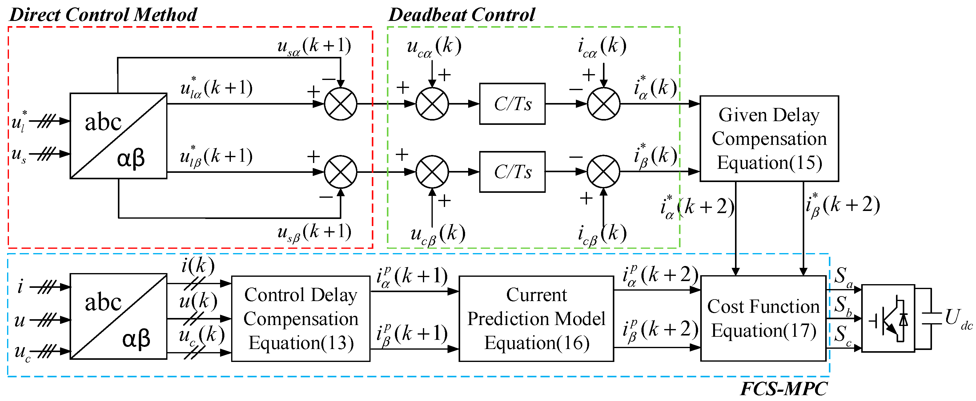
3. The DBDC-FCS-MPC Strategy for SAPF

3.1. The Reference Voltage Generation Mechanism Based on Direct Control

Here, an A-phase voltage in a low-voltage 380 V distribution system is selected as an example for explanation. When the voltage of the power grid is subjected to a temporary swell, sag, or harmonic components, the A-phase load voltage $u_{lA}^{*}$ is the ideal load voltage after SAPF compensation; that is, its amplitude is the standard voltage amplitude, and its phase is consistent with that of the positive sequence phase voltage of the fundamental wave of the A-phase grid. In this case, the relation below can be obtained:

$$u_{lA}^{*}=220\sqrt{2}\sin (\omega t+\phi )$$

(6)

Before compensation, the A-phase grid shows a non-standard voltage amplitude and an inconsistent phase with the positive sequence phase voltage of the fundamental wave of the A-phase grid voltage. Thus, the following equation can be obtained:

$$u_{sA}=\sqrt{2}U\sin (\omega t+\phi )$$

(7)

where $U$ represents the phase voltage of the grid under abnormal conditions. According to Equations (6) and (7), the expression for the reference voltage to be compensated in phase A can be obtained as

$$u_{hA}=u_{lA}^{*}-u_{sA}$$

(8)

In the above expression, $u_{lA}^{*}$ is the ideal load voltage, which is a known constant, and $u_{sA}$ refers to the actual power grid voltage, which can be obtained through sampling.

In a short system control period, the components that may result in system delay, such as the PLL and low-pass filter, are not applied under direct control. The voltage reference signal of the SAPF to be compensated can be obtained directly based on Equation (8) above, which simplifies the control algorithm.

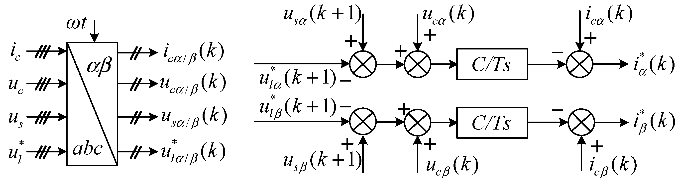
3.2. The Reference Current Generation Mechanism Based on DBC

Based on the DBC principle [23,24], Equation (5) is discretized by the forward Euler method within one sampling period $T_s$, and the predicted output voltage of the SAPF within the $(k+1)T_s$ period is as follows:

$${\mathit{u}}_c^p(k+1)={\mathit{u}}_c(k)+\frac{T_s}{C}[\mathit{i}(k)-{\mathit{i}}_c(k)]$$

(9)

where the upper index $p$ represents the predicted value; $\mathit{y}(k)$ represents the value of the variable $\mathit{y}$ in the $k{T}_s$ period; and $\mathit{y}(k+1)$ is the value of the variable $\mathit{y}$ in the $(k+1)T_s$ period.

If the predicted SAPF output voltage $u_c^p(k+1)$ is assumed to be equal to the amplitude of the voltage to be compensated $u_h(k+1)$ with opposite polarity, the SPAF can compensate for the load voltage if the compensated voltage is fully tracked within one sampling cycle, as follows:

$${\mathit{u}}_h(k+1)=-{\mathit{u}}_c^p(k+1)$$

(10)

As mentioned in Section 3.1, the voltage to be compensated in the $(k+1)T_s$ period is as follows:

$${\mathit{u}}_h(k+1)={\mathit{u}}_l^{*}(k+1)-{\mathit{u}}_s(k+1)$$

(11)

where $u_l^{*}(k+1)$ is a constant, and $u_s(k+1)$ refers to the set three-phase voltage of the system, which can be regarded as a known quantity.

After Equations (10) and (11) are substituted into Equation (9), the reference value of the output current of the inverter in the $k{T}_s$ period can be obtained as follows:

$${\mathit{i}}^{*}(k)={\mathit{i}}_c(k)-\frac{C}{T_s}[{\mathit{u}}_l^{*}(k+1)-{\mathit{u}}_s(k+1)+{\mathit{u}}_c(k)]$$

(12)

According to the above analysis, the generating mechanism of the output current reference value based on DBDC is shown in Figure 3.

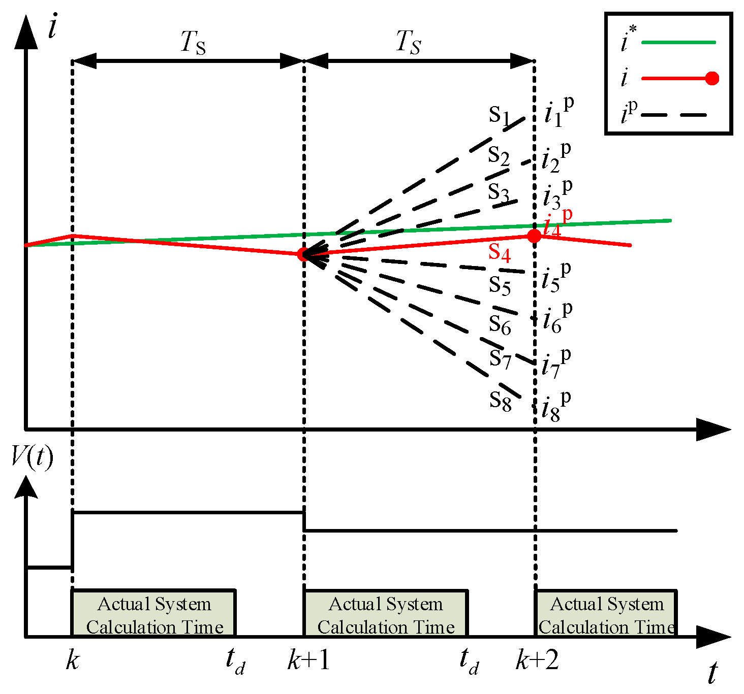
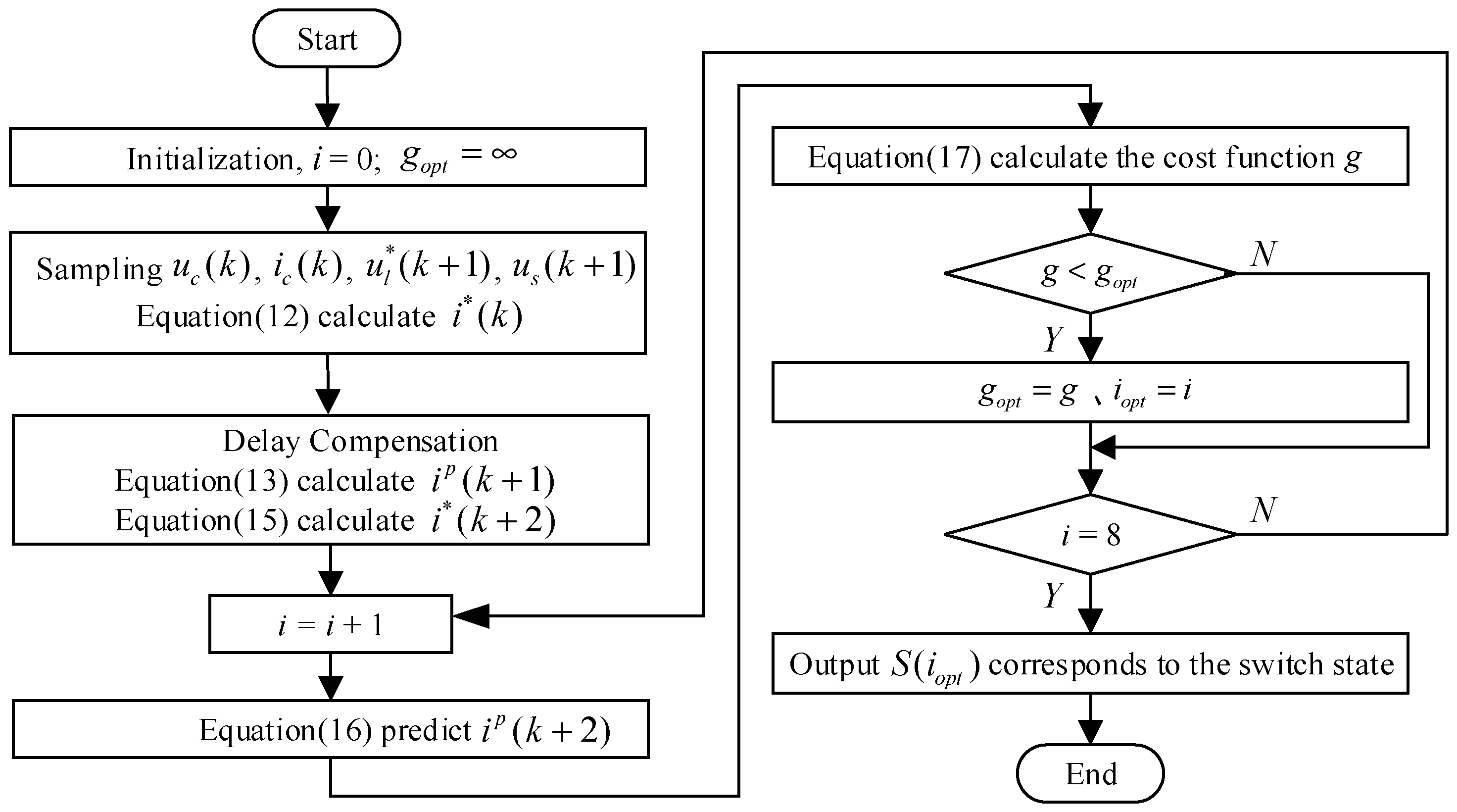
3.3. FCS-MPC of SAPF

After Equation (4) is discretized using the forward Euler method, the prediction model of the inverter output current in the αβ coordinate system can be established, as follows:

$${\mathit{i}}^p(k+1)=(1-\frac{R{T}_s}{L})\mathit{i}(k)+\frac{T_s}{L}[\mathit{u}(k)-{\mathit{u}}_c(k)]$$

(13)

The compensation strategy displayed in Figure 4 is employed to solve the inherent control delay of the digital control system. The optimal vector selected in the previous period is sampled at the time k and applied to obtain the given reference current with Equation (12), and the Lagrange extrapolation method is adopted to compensate to obtain the given value at the time k + 1. Equation (13) is used to compensate for the control delay of the actual value. The predicted value at time k + 1 is substituted into the prediction model to be the actual value in the $(k+1)T_s$ period, and the predicted value at time k + 2 is obtained. Then, the cost function is compared with the given value to determine the optimal control vector.

The given reference current compensation at time k + 1 is as follows:

$${\mathit{i}}^{*}(k+1)=3{\mathit{i}}^{*}(k)-3{\mathit{i}}^{*}(k-1)+{\mathit{i}}^{*}(k-2)$$

(14)

The given reference current compensation at time k + 2 is as follows:

$${\mathit{i}}^{*}(k+2)=6{\mathit{i}}^{*}(k)-8{\mathit{i}}^{*}(k-1)+3{\mathit{i}}^{*}(k-2)$$

(15)

The predicted value at time k + 2 is as follows:

$${\mathit{i}}^p(k+2)=(1-\frac{R{T}_s}{L}){\mathit{i}}^p(k+1)+\frac{T_s}{L}[\mathit{u}(k+1)-{\mathit{u}}_c(k+1)]$$

(16)

To minimize the current tracking error, the cost function can be defined as Equation (17):

$$g={[i_{\alpha }^{*}(k+2)-i_{\alpha }^p(k+2)]}^2+{[i_{\beta }^{*}(k+2)-i_{\beta }^p(k+2)]}^2$$

(17)

Figure 5 demonstrates the block diagram of the DBDC-FCS-MPC for the SAPF proposed in this work, and Figure 6 is the specific flow diagram.

4. Simulation Verification and Experimental Analysis

4.1. Simulation Verification

To verify the effectiveness of the proposed strategy, a system model is built according to the SAPF topology in Figure 1. The double closed-loop vector control under indirect control (Strategy I) [15,32], the DBC-FCS-MPC under indirect control (Strategy II) [33], and the DBDC-FCS-MPC proposed in this work (Strategy III) are compared. The simulation is composed of two parts: the first part aims to compare the dynamic and steady performance of the proposed strategy and the traditional strategy; the second part highlights the superiority of the proposed strategy in compensating for the full-frequency harmonic voltage. The main parameters for the simulation are listed in

Table 1. Main simulation parameters.

Simulation Parameters	Numerical Values
Grid Voltage/Frequency	220 V/50 Hz
Series Transformer Ratio	1:1
Nonlinear Resistive Load	L = 10 mH, R = 30 Ω
Filter Capacitor and Inductor	Lf = 5 mH, Cf = 100 μF, Rf = 2 Ω
DC Voltage	Udc = 700 V
FCS–MPC Control Period	Ts = 83 μs

.

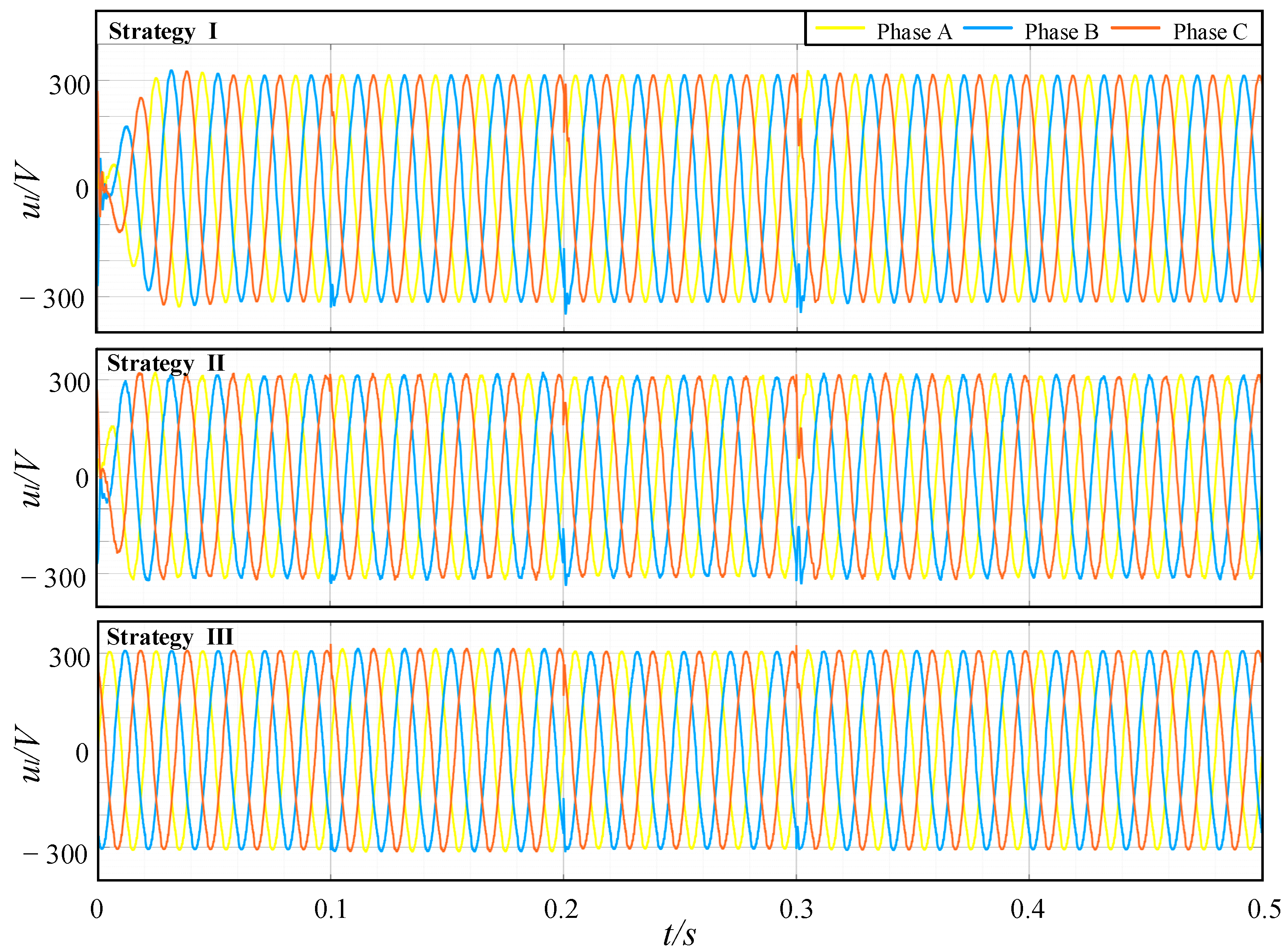
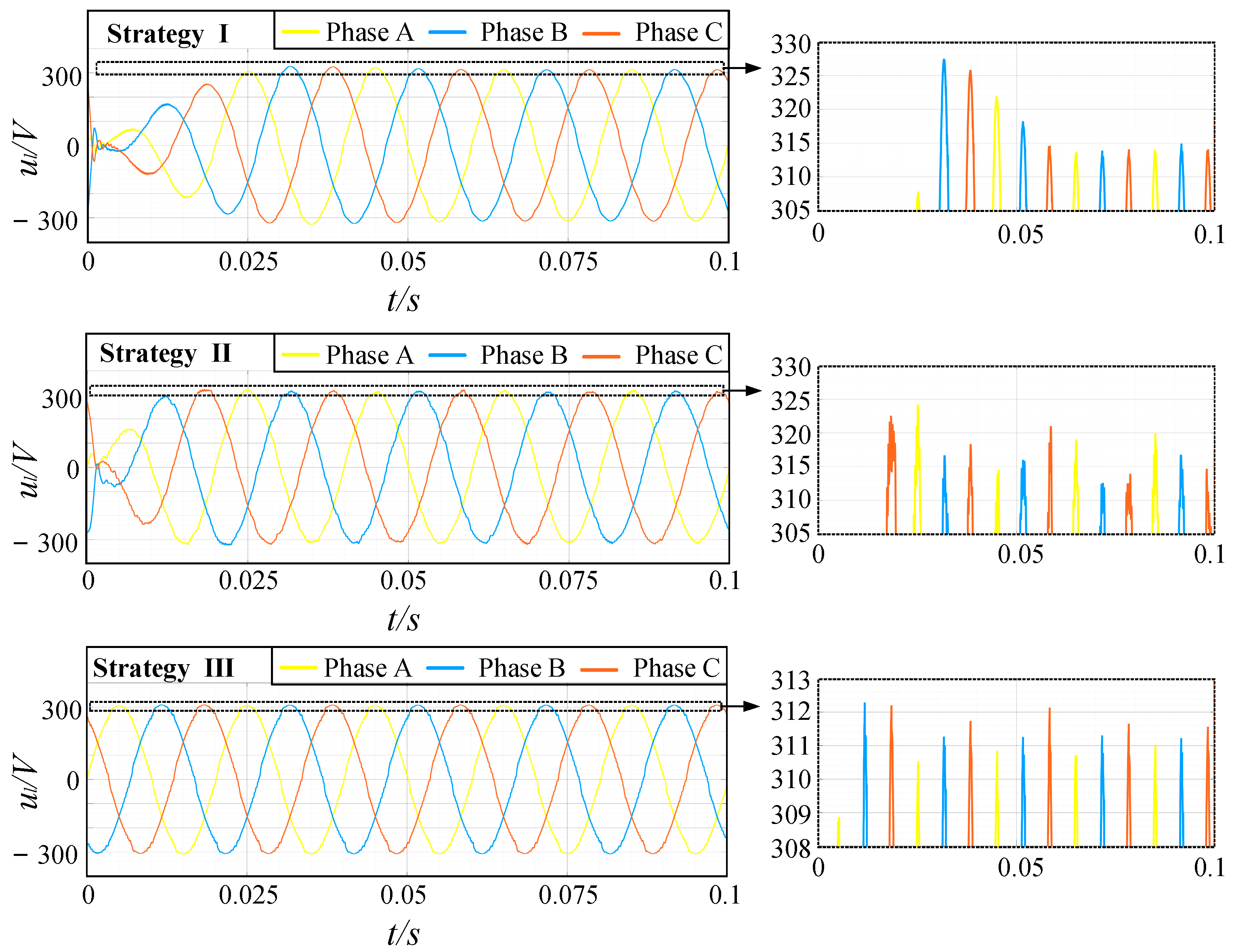
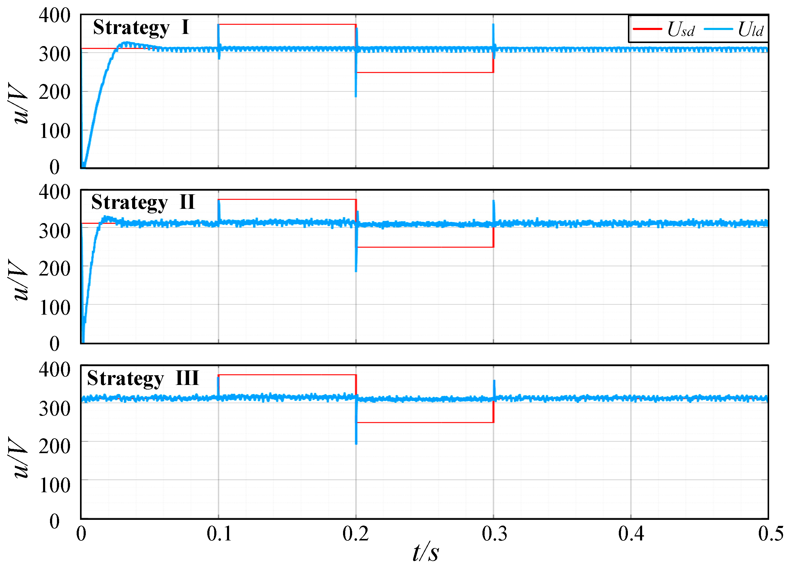
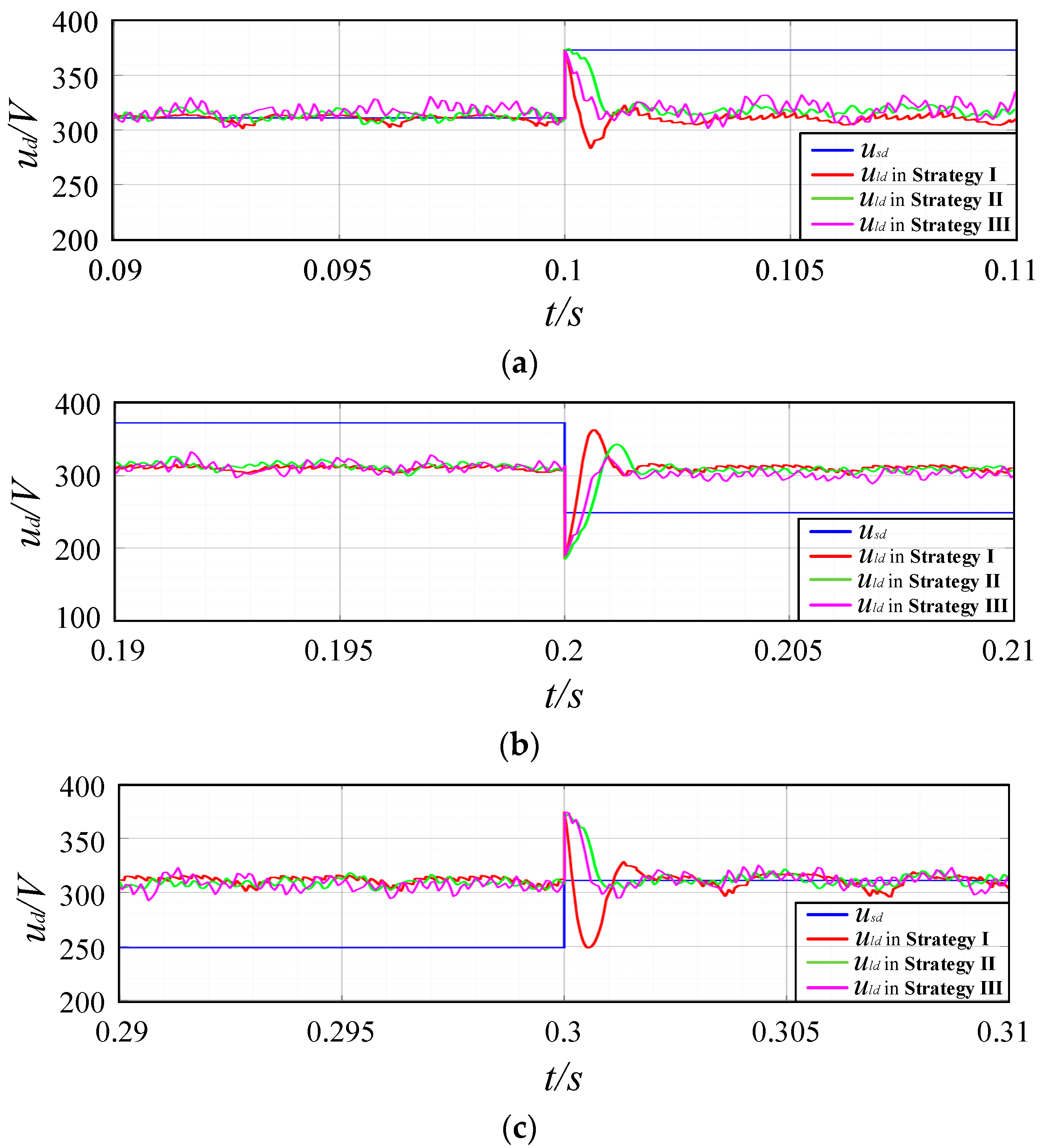
4.1.1. Dynamic and Steady-State Performance of the Voltage Amplitude Compensation

This work assumes that the grid voltage remains normal between 0 and 0.1 s, a 20% temporary swell occurs at 0.1–0.2 s, a 20% temporary sag occurs at 0.2–0.3 s, sudden changes in load occur at 0.3 s, and it returns to normal after 0.4 s. The mutating load is set as an uncontrolled rectifier bridge with resistive load, where L₁ = 1 mH, and R₁ = 10 Ω.

Figure 7 demonstrates the load voltage waveforms after compensation under the three control strategies. It is observed that the SAPF can compensate for the load voltage under all three control strategies, so that it maintains the sinusoidal waveforms and amplitudes at about 311 V. In addition, the detailed plots of the load voltage at 0–0.1 s are shown in Figure 8. It can clearly be seen that the response time of the system becoming stable for Strategy I and Strategy II under indirect control is about 25 ms and 20 ms with a certain lag, while that for Strategy III is invisible. It suggests that compared with indirect control, the direct control employed in this work can effectively improve the dynamic response capability of the system without affecting the compensation performance. Furthermore, Figure 8 gives a zoomed-in view of the load voltage when the amplitude is stable. It shows that after compensation by the proposed control Strategy III, the load voltage can be stabilized at 311 V, while Strategy I and Strategy II have certain inaccuracy, and the amplitude is stable above and below 315 V. This proves the superiority of the proposed strategy in terms of compensating for voltage amplitude.

With the three control strategies, the A-phase voltage to be compensated $u_{ha}^{*}$ for the temporary swell and sag conditions that exist on the grid between 0.1 and 0.3 s are fitted with the actual output value $u_{ca}$ of the SAPF, as shown in Figure 9. The figure suggests that the two voltage waveforms under the three control strategies almost coincide, and the output voltage of the SAPF can track the voltage to be compensated in real time. Compared with Strategy I, Strategy III can track and control the reference current via the FCS-MPC replacement current loop and improve the current setting using the DBC replacement voltage loop. In this way, it effectively reduces the burr of the SAPF output voltage, tracks the voltage to be compensated more accurately, and improves the compensation performance. Meanwhile, the tracking effect between Strategy II and Strategy III exhibits no significant difference when the compensated voltage is subjected to a temporary swell and sag. However, under the harmonic voltage, the SAPF output voltage in Strategy II is slightly larger than the voltage to be compensated, resulting in a smaller load voltage after compensation, which affects the control performance.

The d-axis DC components of the grid voltage before compensation $u_{sd}$ and the load voltage after compensation $u_{ld}$ are as shown in Figure 10. It can be demonstrated that all three strategies are successful in maintaining stable load voltage under the conditions of a temporary swell and sag of the grid voltage and sudden load changes. In addition, the system takes a certain amount of time to stabilize with both Strategy I and Strategy II, whereas under the proposed Strategy III, the system can be stabilized at start-up without any extra time delay.

Figure 11 displays the details of the changes in grid and load voltages over a short period of time for the three sudden changes in working conditions described above. It can be noticed that the load voltage under the traditional Strategy I fluctuates to a certain extent when the grid working conditions change, and there is a higher amount of overshoot. The fluctuation of the load voltage change under the proposed Strategy III is lower, and the time to stabilize is shorter than the remaining two strategies, highlighting the better dynamic compensation performance of the proposed control strategy.

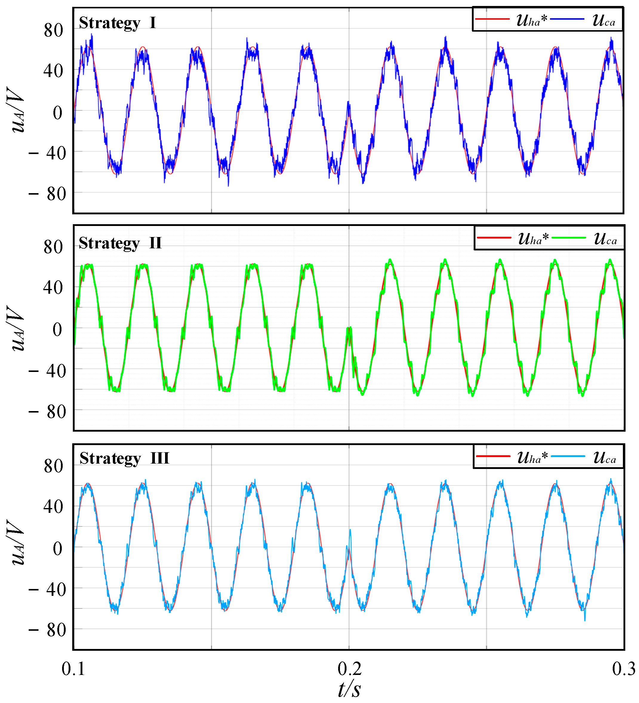
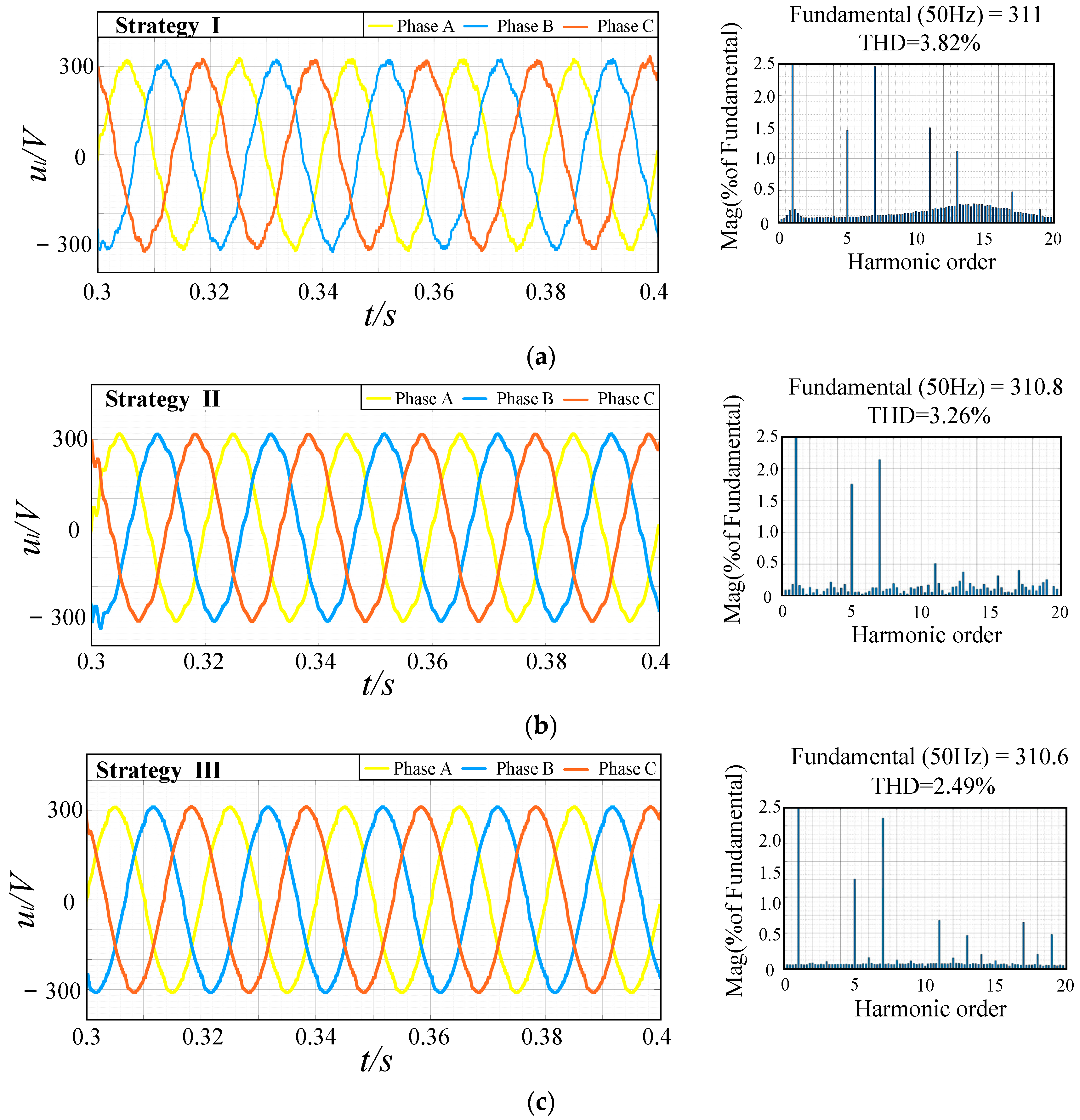
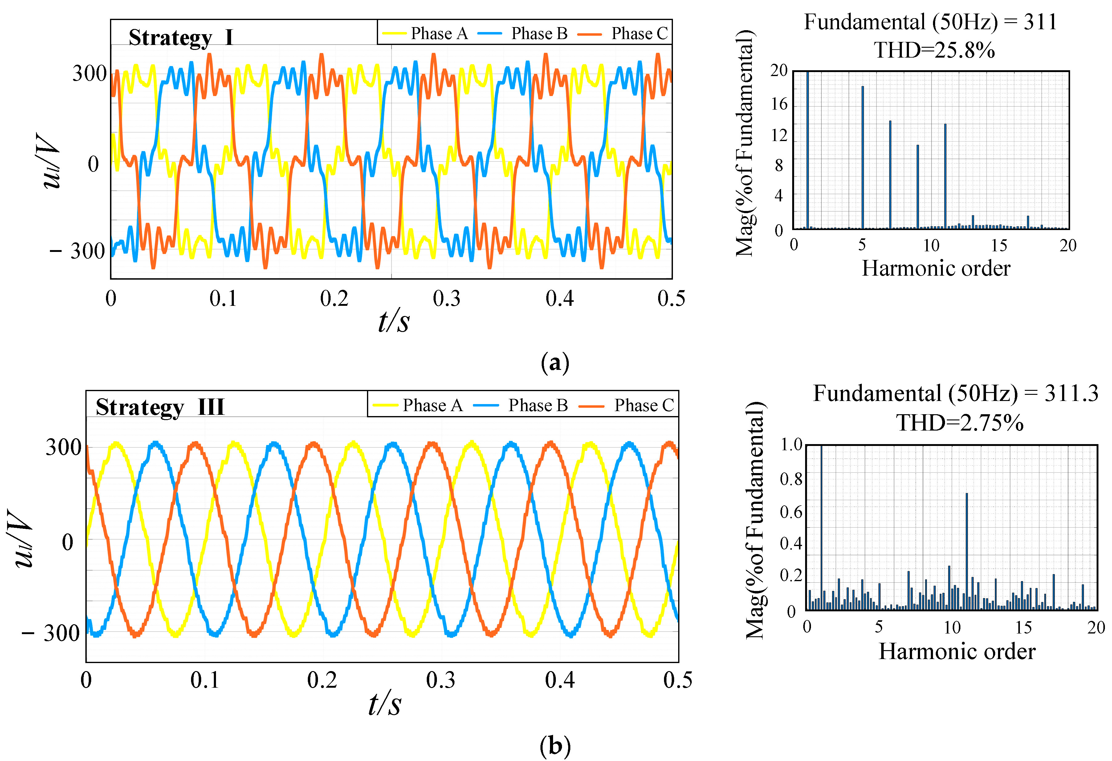
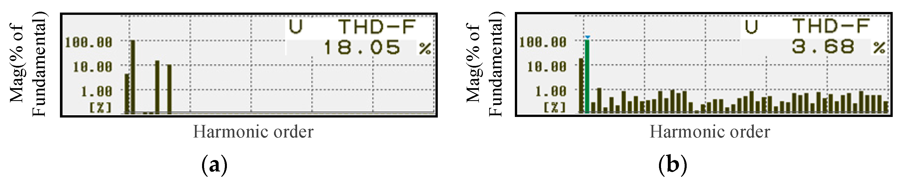
4.1.2. Compensation Performance of the Full-Frequency Harmonic Voltage

Assuming that the fifth harmonics with a 15% positive sequence and the seventh harmonics with a 10% negative sequence are observed in the grid voltage within 0.3–0.4 s, the load voltages compensated by the three control strategies are illustrated in Figure 12. It shows that compared with Strategy I, Strategy III is superior in voltage compensation and performs better in the load voltage waveform after compensation under a temporary voltage swell and sag. It also provides the total harmonic distortion (THD) values for the load voltage after compensation under three control strategies for the above harmonic condition in Figure 12. It is known that the THD values of the load voltage are 3.82%, 3.26%, and 2.49%, respectively, which are all less than 5%, meeting the network requirements for harmonic voltage stipulated in IEC61000-2-2 (an international standard) [34]. The comparative analysis reveals that Strategy III presents an obviously better compensation effect on the fifth and seventh harmonics without generating a large number of harmonics in other frequencies, proving the superiority of the proposed strategy. Such a result verifies the effectiveness of the strategy proposed in this work to compensate for harmonic voltages.

The QPR controller is arranged for closed-loop control in Strategy I for the non-static error tracking of harmonic AC signals, but the controller with fixed parameters can only achieve effective gain for signals with specific frequencies. However, the QPR controller without parameter tuning cannot track the harmonic signals with other frequencies accurately. It is assumed, in this work, that within 0.3–0.4 s, the harmonics of grid voltage change from the 5th harmonics with a 15% positive sequence and the 7th harmonics with a 10% negative sequence to the 9th harmonics with a 20% positive sequence and the 11th harmonics with a 10% negative sequence, respectively. Figure 13 displays the load voltage waveforms compensated by Strategies I and III under the conditions assumed above. It can be observed that even with the 9th and 11th harmonics voltages, the QPR controller in Strategy I can only track the 5th and 7th harmonics voltages if the parameters are not adjusted, which affects the subsequent control link, resulting in poor compensation and large distortion of load voltage. In contrast, the proposed Strategy III can track the AC signals without the traditional controller and effectively suppress the 9th and 11th harmonic voltages, which compensates for the full-frequency harmonics, further proving the superiority of the proposed strategy.

The harmonic distortion rates within 0.3–0.4 s under the two control strategies are measured, as given in Figure 13. The THD value of the grid voltage is 22.36% when the 9th and 11th harmonics are observed in the system, and it becomes 25.8% and 2.75% after the compensation of the two strategies, respectively. Meanwhile, the compensation effects of Strategy III on the 9th and 11th harmonics are obviously better than those of Strategy I, which is supported by greatly reduced harmonic content. It, again, verifies the advantage of the proposed Strategy III to suppress the full-frequency harmonic voltage distortion.

To ensure the effectiveness of the comparative analysis, the equivalent sampling frequencies of the three control strategies are all set to 12 kHz, and the equivalent switching frequency of the IGBT in the main circuit is counted. The compensation effects under the three control strategies are quantitatively compared, and the specific data are shown in

Table 2. Quantitative comparison of the effects of three control strategies.

Contrast Items	Strategy I	Strategy II	Strategy III
THD before compensation (%)	18.03	18.03	18.03
THD after compensation (%)	3.82	3.26	2.49
Actual sampling frequency (kHz)	2	12	12
Equivalent switching frequency (kHz)	2	2.6	3.4

. Analysis of the table reveals that the proposed control strategy exhibits the optimal compensation effect under the same equivalent sampling frequency.

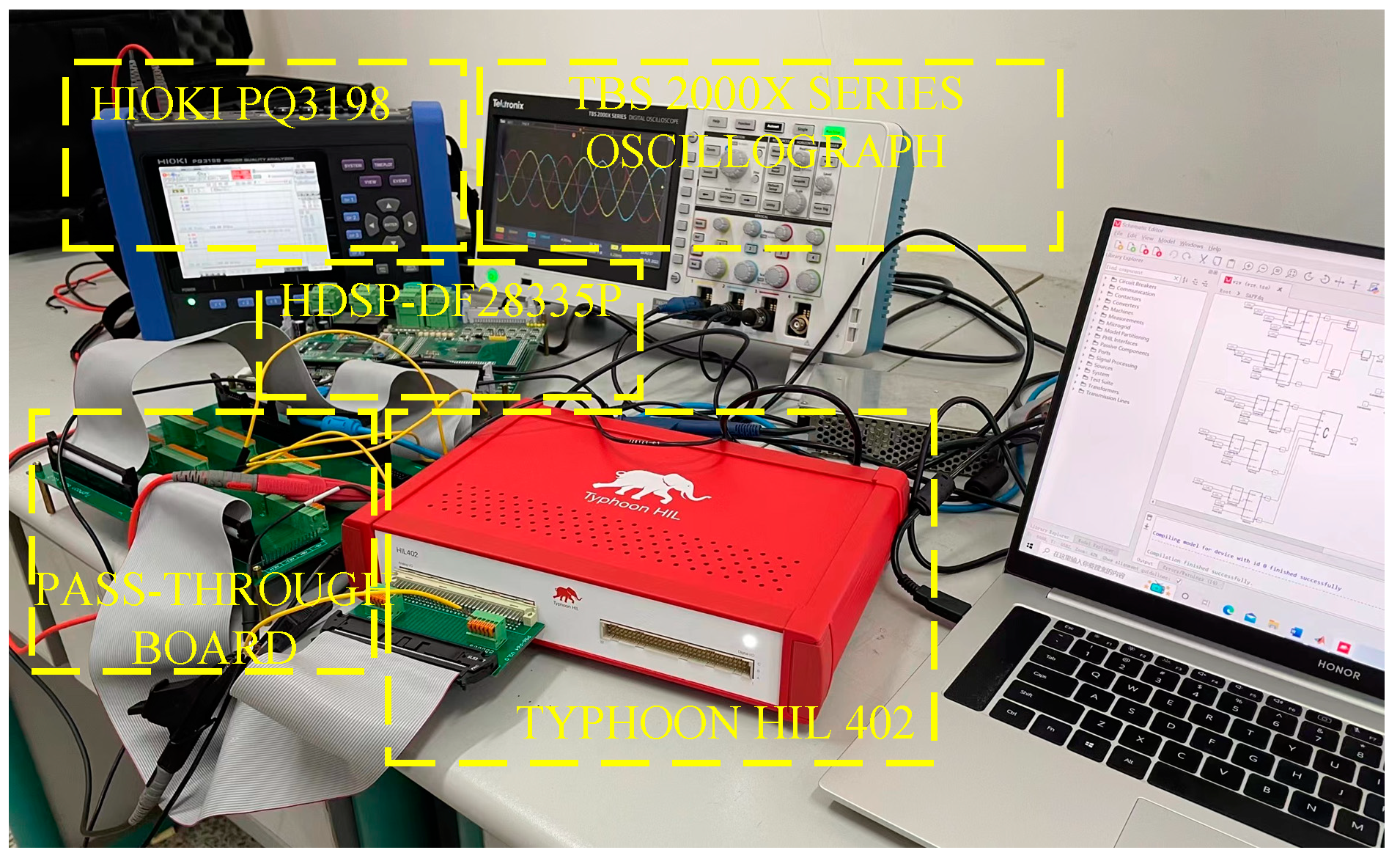
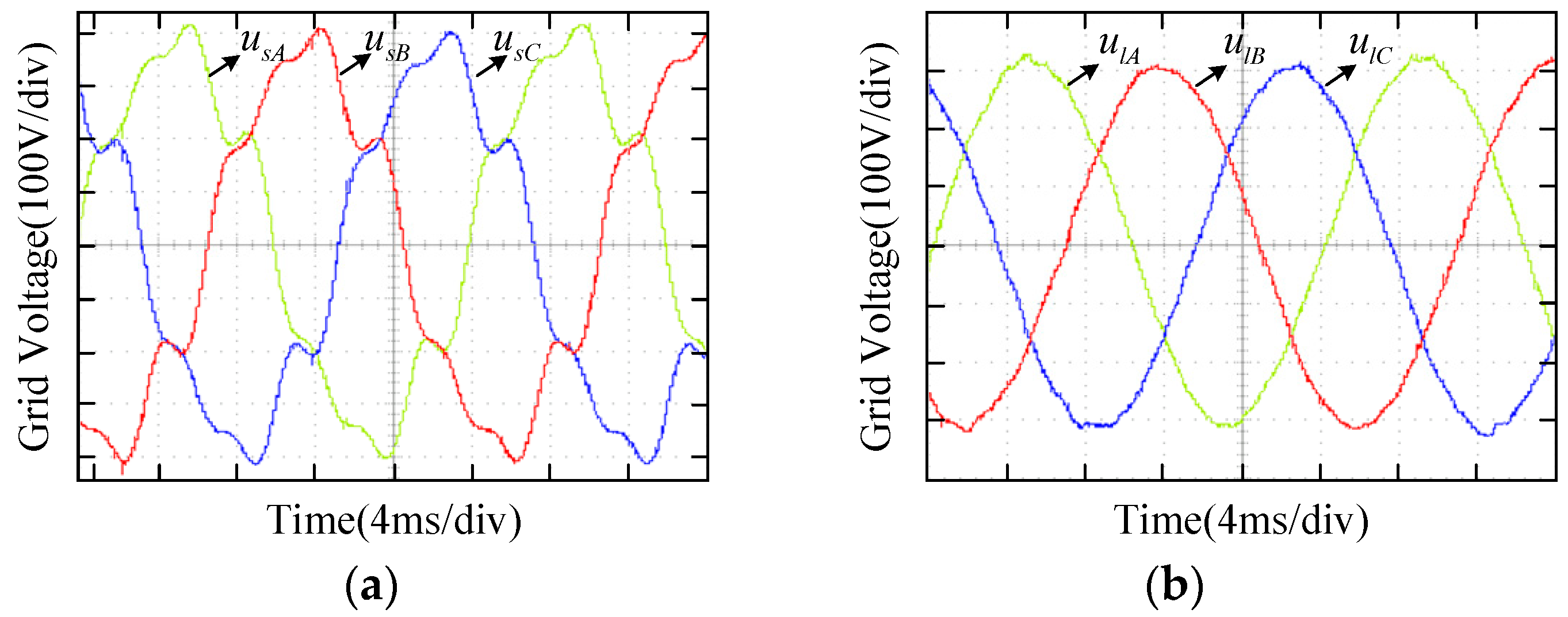
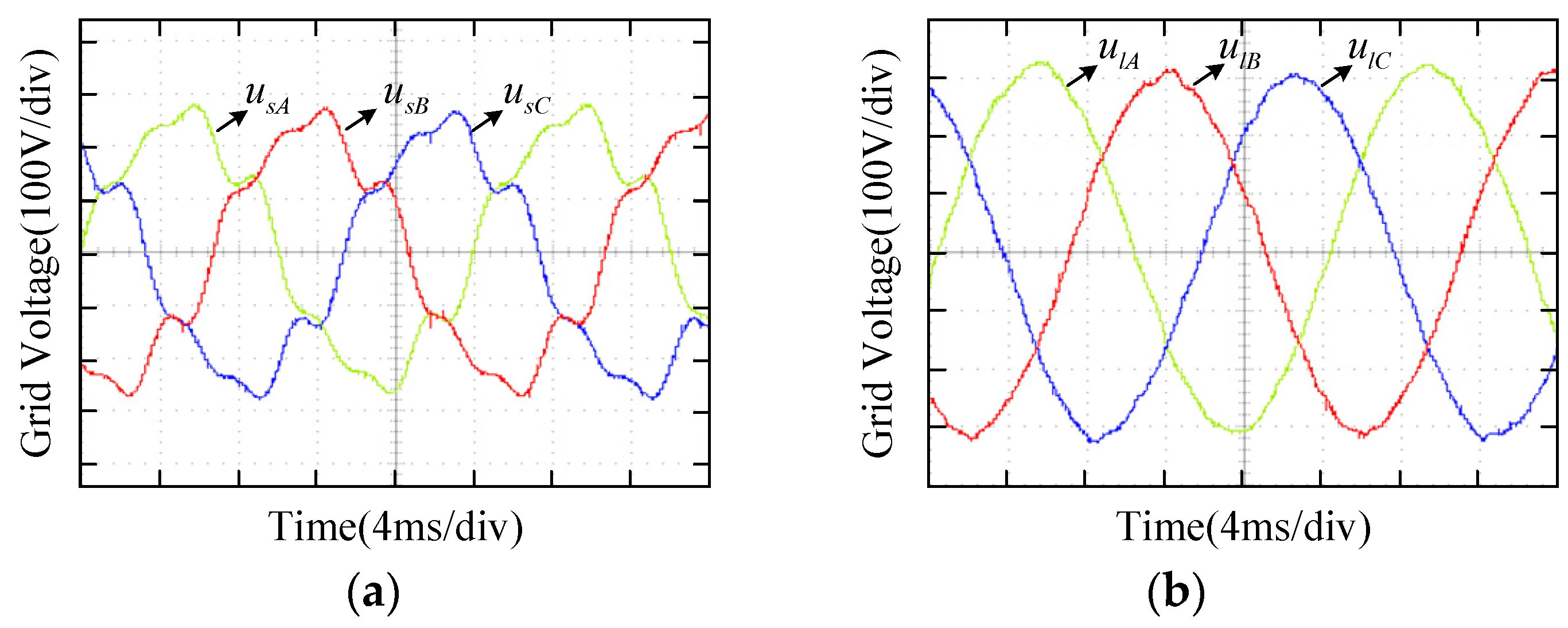
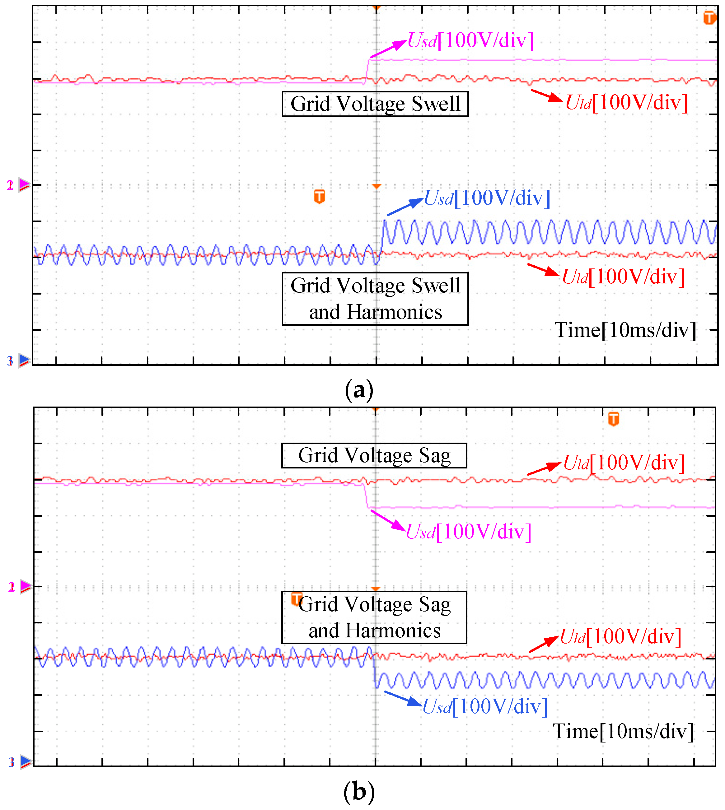
4.2. Experimental Analysis

In addition, a semi-physical experimental platform is built, as shown in Figure 14, to verify the effectiveness of the proposed strategy further. The controller HDSP-DF28335P is employed to output the pulses. The main circuit of the model is built on Typhoon HIL 402, and the voltage harmonic distortion rate is calculated with the HIOKI power quality analyzer PQ3198. The experiment mainly verifies the SAPF compensation performance of the proposed DBDC-FCS-MPC strategy under the conditions of a temporary swell, sag, and harmonic voltage. The main parameters are set as listed in Table 1.

Figure 15 exhibits the experimental results of the grid voltage under a temporary swell (20%) and a harmonic (18%). It shows that the load voltage in Figure 15b can be compensated as a sinusoidal wave with a constant amplitude and 311 V under the DBDC-FCS-MPC strategy, although there are some surges and distortions in the grid voltage due to the temporary swell and harmonics. Figure 16 illustrates the experimental results when the grid voltage shows a transient sag (20%) and a harmonic (18%), which supports that the proposed strategy still shows a good compensation effect. The THD rate of voltage is measured and analyzed, as demonstrated in Figure 17, which is 18.05% before compensation and is reduced to 3.68% after compensation. It means that the contents of the fifth and seventh harmonic voltages are greatly reduced, which verifies the effectiveness of the control strategy proposed in this work.

The d-axis components of the grid and load voltages are measured for the three working conditions mentioned above, as shown in Figure 18. As can be seen from Figure 18a, when the grid voltage has temporary swell and harmonic conditions, the d-axis component of the load voltage can be maintained at around 311 V after compensation by Strategy III, with less fluctuation. In the same way, Figure 18b shows that the proposed strategy can still complete the voltage compensation function and maintain stability when the grid voltage is transient and contains harmonics.

5. Conclusions

A DBDC-FCS-MPC strategy is proposed to solve the system delay caused by the PLL and harmonic detection in the SAPF with traditional indirect control. Firstly, with the idea of direct compensation control, the voltage reference signals are directly generated based on the ideal load voltage and actual grid voltage, without a PLL and harmonic detection. It solves harmonic detection and improves the dynamic response performance of the system with a dynamic response time of less than 20 ms. Secondly, based on the DBC principle and the FCS-MPC principle, the reference current generation mechanism of the SAPF under an αβ coordinate system is derived and established, and a DBDC-FCS-MPC system is constructed. In this way, it avoids the complex coordinate transformation and cross coupling in voltage outer loop control, further improves the dynamic performance of the system, and effectively suppresses the full-frequency harmonic voltage. The simulation and experimental results disclose that the proposed DBDC-FCS-MPC strategy can compensate for the voltage effectively without harmonic detection, a PLL, a closed-loop controller, and PWM, ensuring a stable voltage amplitude within the standard range, and reducing the THD rate by 1.33% for voltage harmonic compensation compared with the traditional double closed-loop control strategy.

References

1. Turovi, R.; Dragan, D.; Goji, G.; Petrovi, V.-B.; Gajic, D.-B.; Stanisavljevi, A.-M.; Kati, V.-A. An End-to-End Deep Learning Method for Voltage Sag Classification. Energies 2022, 15, 2898. [Google Scholar] [CrossRef]
2. Garnica López, M.A.; de Vicuña, J.L.G.; Miret, J.; Castilla, M.; Guzmán, R. Control Strategy for Grid-Connected Three-Phase Inverters During Voltage Sags to Meet Grid Codes and to Maximize Power Delivery Capability. IEEE Trans. Power Electron. 2018, 33, 9360–9374. [Google Scholar] [CrossRef] [Green Version]
3. Wang, L.; Lam, C.-S.; Wong, M.-C. Analysis, Control, and Design of a Hybrid Grid-Connected Inverter for Renewable Energy Generation with Power Quality Conditioning. IEEE Trans. Power Electron. 2018, 33, 6755–6768. [Google Scholar] [CrossRef]
4. Choi, W.; Lee, W.; Han, D.; Sarlioglu, B. New Configuration of Multifunctional Grid-Connected Inverter to Improve Both Current-Based and Voltage-Based Power Quality. IEEE Trans. Ind. Appl. 2018, 54, 6374–6382. [Google Scholar] [CrossRef]
5. Fujita, H.; Akagi, H. An Approach to Harmonic Current-Free AC/DC Power Conversion for Large Industrial Loads: The Integration of a Series Active Filter with a Double-series Diode Rectifier. IEEE Trans. Ind. Appl. 1997, 33, 1233–1240. [Google Scholar] [CrossRef] [Green Version]
6. Can, E. The Levels Effect of the Voltage Generated by an Inverter with Partial Source on Distortion. Int. J. Electron. 2020, 107, 1414–1435. [Google Scholar] [CrossRef]
7. Radzi, M.A.M.; Rahim, N.-A. Neural Network and Bandless Hysteresis Approach to Control Switched Capacitor Active Power Filter for Reduction of Harmonics. IEEE Trans. Ind. Electron. 2009, 56, 1477–1484. [Google Scholar] [CrossRef]
8. Fereidouni, A.; Masoum, M.A.S.; Smedley, K.-M. Supervisory Nearly Constant Frequency Hysteresis Current Control for Active Power Filter Applications in Stationary Reference Frame. IEEE Power Energy Technol. Syst. J. 2016, 3, 1–12. [Google Scholar] [CrossRef]
9. Gong, C.; Sou, W.-K.; Lam, C.-S. Design and Analysis of Vector Proportional–Integral Current Controller for LC-Coupling Hybrid Active Power Filter with Minimum DC-Link Voltage. IEEE Trans. Power Electron. 2021, 36, 9041–9056. [Google Scholar] [CrossRef]
10. Alam, S.-J.; Arya, S.-R. Control of UPQC Based on Steady State Linear Kalman Filter for Compensation of Power Quality Problems. Chin. J. Electr. Eng. 2020, 6, 52–65. [Google Scholar] [CrossRef]
11. Can, E.; Sayan, H.-H. PID and Fuzzy Controlling Three Phase Asynchronous machine by Low Level DC Source Three Phase Inverter. Teh. Vjesn. Tech. Gaz. 2016, 23, 753–760. [Google Scholar]
12. Pandove, G.; Singh, M. Robust Repetitive Control Design for a Three-Phase Four Wire Shunt Active Power Filter. IEEE Trans. Ind. Inform. 2019, 15, 2810–2818. [Google Scholar] [CrossRef]
13. Geng, H.; Zheng, Z.; Zou, T.; Chu, B.; Chandra, A. Fast Repetitive Control with Harmonic Correction Loops for Shunt Active Power Filter Applied in Weak Grid. IEEE Trans. Ind. Appl. 2019, 55, 3198–3206. [Google Scholar] [CrossRef]
14. Wang, H.; Wu, X.; Zheng, X.; Yuan, X. An Improved Hysteresis Current Control Scheme During Grid Voltage Zero-Crossing for Grid-Connected Three-Level Inverters. IET Power Electron. 2021, 14, 1946–1959. [Google Scholar] [CrossRef]
15. Sou, W.-K.; Chao, C.-W.; Gong, C.; Lam, C.-S.; Wong, C.-K. Analysis, Design, and Implementation of Multi-Quasi-Proportional-Resonant Controller for Thyristor-Controlled LC-Coupling Hybrid Active Power Filter (TCLC-HAPF). IEEE Trans. Ind. Electron. 2022, 69, 29–40. [Google Scholar] [CrossRef]
16. Dragičević, T.; Zheng, C.; Rodriguez, J.; Blaabjerg, F. Robust Quasi-Predictive Control of LCL-Filtered Grid Converters. IEEE Trans. Power Electron. 2020, 35, 1934–1946. [Google Scholar] [CrossRef]
17. Jian, L.; Li, X.; Zhu, J.; Zhang, H.; Li, F. Dual Closed-Loops Current Controller for a 4-Leg Shunt APF Based on Repetitive Control. Int. J. Electron. 2019, 106, 349–364. [Google Scholar] [CrossRef]
18. Can, E.; Sayan, H.-H. The Increasing Harmonic Effects of SSPWM Multilevel Inverter Controlling Load Currents Investigated on Modulation Index. Teh. Vjesn. Tech. Gaz. 2017, 24, 397–404. [Google Scholar]
19. Shu, Z.; Lin, H.; Zhang, Z.; Yin, X.; Zhou, Q. Specific Order Harmonics Compensation Algorithm and Digital Implementation for Multi-level Active Power Filter. IET Power Electron. 2016, 10, 525–535. [Google Scholar] [CrossRef]
20. Can, E.; Sayan, H.-H. A Novel SSPWM Controlling Inverter Running Nonlinear Device. Electr. Eng. 2018, 100, 39–46. [Google Scholar] [CrossRef]
21. Wang, Z.; Chai, J.; Sun, X.; Lu, H. Predictive Deviation Filter for Deadbeat Control. IET Electr. Power Appl. 2020, 14, 1041–1049. [Google Scholar] [CrossRef]
22. Xue, C.; Ding, L.; Tian, H.; Li, Y. Multirate Finite-Control-Set Model Predictive Control for High Switching Frequency Power Converters. IEEE Trans. Ind. Electron. 2022, 69, 3382–3392. [Google Scholar] [CrossRef]
23. Vazquez, S.; Zafra, E.; Aguilera, R.-P.; Geyer, T.; Leon, J.-I.; Franquelo, L.-G. Prediction Model with Harmonic Load Current Components for FCS-MPC of an Uninterruptible Power Supply. IEEE Trans. Power Electron. 2022, 37, 322–331. [Google Scholar] [CrossRef]
24. Long, B.; Zhu, Z.; Yang, W.; Chong, K.-T.; Rodríguez, J.; Guerrero, J.-M. Gradient Descent Optimization Based Parameter Identification for FCS-MPC Control of LCL-Type Grid Connected Converter. IEEE Trans. Ind. Electron. 2022, 69, 2631–2643. [Google Scholar] [CrossRef]
25. Mohammed, A.; Paolo, M.; Pooya, D. Harmonics Mitigation and Non-ideal Voltage Compensation Utilising Active Power Filter Based on Predictive Current Control. IET Power Electron. 2020, 13, 2782–2793. [Google Scholar]
26. Ferreira, S.-C.; Gonzatti, R.-B.; Pereira, R.-R.; da Silva, C.-H.; da Silva, L.E.B.; Lambert-Torres, G. Finite Control Set Model Predictive Control for Dynamic Reactive Power Compensation with Hybrid Active Power Filters. IEEE Trans. Ind. Electron. 2018, 65, 2608–2617. [Google Scholar] [CrossRef]
27. Panten, N.; Hoffmann, N.; Fuchs, F.-W. Finite Control Set Model Predictive Current Control for Grid-Connected Voltage-Source Converters with LCL Filters: A Study Based on Different State Feedbacks. IEEE Trans. Power Electron. 2016, 31, 5189–5200. [Google Scholar] [CrossRef]
28. Wang, W.; Liu, C.; Zhao, H.; Song, Z. Improved Deadbeat-Direct Torque and Flux Control for PMSM With Less Computation and Enhanced Robustness. IEEE Trans. Ind. Electron. 2023, 70, 2254–2263. [Google Scholar] [CrossRef]
29. Yao, Y.; Huang, Y.; Peng, F.; Dong, J.; Zhang, H. An Improved Deadbeat Predictive Current Control with Online Parameter Identification for Surface-Mounted PMSMs. IEEE Trans. Ind. Electron. 2020, 67, 10145–10155. [Google Scholar] [CrossRef] [Green Version]
30. Karbasforooshan, M.-S.; Monfared, M. An Improved Reference Current Generation and Digital Deadbeat Controller for Single-Phase Shunt Active Power Filters. IEEE Trans. Power Deliv. 2020, 35, 2663–2671. [Google Scholar] [CrossRef]
31. Sou, W.-K.; Choi, W.-H.; Chao, C.-W.; Lam, C.-S.; Gong, C.; Wong, C.-K.; Wong, M.-C. A Deadbeat Current Controller of LC-Hybrid Active Power Filter for Power Quality Improvement. IEEE J. Emerg. Sel. Top. Power Electron. 2020, 8, 3891–3905. [Google Scholar] [CrossRef]
32. Parul, C.; Singh, G. Fault Mitigation Through Multi Converter UPQC with Hysteresis Controller in Grid Connected Wind System. J. Ambient Intell. Humaniz. Comput. 2020, 11, 5279–5295. [Google Scholar]
33. Wang, G.; Gao, X.; Wu, Z.; Guo, J.; Liu, Z. Research on a Finite Control Set Model Predictive Control Strategy for Series APF Based on Deadbeat Outer Loop Control. Power Syst. Clean Energy 2022, 38, 15–23. [Google Scholar]
34. CENELEC—EN 61000-2-2; Electromagnetic Compatibility (EMC)-Part 2-2: Environment-Compatibility Levels for Low-Frequency Conducted Disturbances and Signalling in Public Low-Voltage Power Supply Systems. European Committee for Electrotechnical Standardization (CENELEC): Brussels, Belgium, 2002.
Figure 1. Three-phase two-level SAPF topology.
Energies 16 02507 g001
Figure 2. SAPF single-phase equivalent circuit diagram.
Energies 16 02507 g002
Figure 3. Reference current generation mechanism based on DBDC.
Energies 16 02507 g003
Figure 4. Predictive current control diagram after delay compensation.
Energies 16 02507 g004
Figure 5. Control block diagram of SAPF system based on the DBDC-FCS-MPC strategy.
Energies 16 02507 g005
Figure 6. Flow of the DBDC-FCS-MPC strategy.
Energies 16 02507 g006
Figure 7. Load voltage under temporary swell, sag, and sudden load change conditions.
Energies 16 02507 g007
Figure 8. Detail of load voltage at 0–0.1 s.
Energies 16 02507 g008
Figure 9. Comparison of A-phase output voltage tracking effect.
Energies 16 02507 g009
Figure 10. The d-axis DC components of the grid voltage and load voltage.
Energies 16 02507 g010
Figure 11. Voltage details at change in working conditions. (a) Instantaneous grid voltage swell; (b) instantaneous grid voltage sag; (c) instantaneous sudden changes in load.
Energies 16 02507 g011
Figure 12. Load voltage after compensation under harmonic conditions. (a) Load voltage under Strategy I; (b) load voltage under Strategy II; (c) load voltage under Strategy III.
Energies 16 02507 g012
Figure 13. Load voltage after compensation of harmonics of different frequencies. (a) Load voltage after compensation of the 9th and 11th harmonics via Strategy I; (b) load voltage after compensation of the 9th and 11th harmonics via Strategy III.
Energies 16 02507 g013
Figure 14. Semi-physical experimental platform.
Energies 16 02507 g014
Figure 15. Temporary swell and harmonic conditions. (a) Grid voltage before compensation; (b) load voltage after compensation.
Energies 16 02507 g015
Figure 16. Temporary sag and harmonic conditions. (a) Grid voltage before compensation; (b) load voltage after compensation.
Energies 16 02507 g016
Figure 17. The THD rate of voltage based on Strategy III. (a) Grid voltage before compensation; (b) load voltage after compensation.
Energies 16 02507 g017
Figure 18. d-axis voltage at change in working conditions. (a) Grid voltage swell and harmonics. (b) Grid voltage sag and harmonics.
Energies 16 02507 g018