UAV Photogrammetry Application for Determining the Influence of Shading on Solar Photovoltaic Array Energy Efficiency

Abstract

The field of solar photovoltaic (PV) plants has seen significant growth in recent years, with an increasing number of installations being developed worldwide. However, despite advancements in technology and design, the impact of shading on the performance of PV plants remains an area of concern. Accurate 3D models produced using unmanned aerial vehicle (UAV) photogrammetry can provide aid to evaluate shading from nearby surroundings and to determine the potential of a site for electricity production via solar PV plants. The main objective of this paper is to address the problem of shadows significantly reducing energy yield in solar PV plants by proposing a methodology that aims at assessing the shading effects on PV systems and determining the optimal configuration for a PV module array using an accurate digital environment 3D model built using UAV photogrammetry. A high-level-of-detail 3D model allows us to evaluate possible obstacles for PV module array construction and accurately recreate the proximities that can cast shadows. The methodology was applied to grid-connected PV systems in Kaunas, Lithuania. The results of the case study show that electricity production in PV modules is highest at a 15° tilt angle when the distance between PV rows is 1.25 m. The proposed methodology gives an 11% difference in PV yield due to shading compared with other tools that do not include shading. This study also highlights that at least 30% financing support is necessary for solar PV plants to be economically attractive, resulting in a payback of 9 years and an internal rate of return of 8%. Additionally, this study can help optimize the design and layout of PV systems, making them more efficient and cost-effective.

1. Introduction

Currently, energy production from renewable energy sources (RESs) is rapidly gaining popularity, as it reduces dependency on fossil fuels and greenhouse gas emissions. One way to produce energy is to generate electricity in solar photovoltaic (PV) power plants (PPs). The total installed capacity of solar PPs in the European Union (EU) has increased from 16 GW in 2009 [1] to 159 GW in 2021 [2]. This increase has been driven by a steady fall in PV module prices and the increasing efficiency of electricity generation as technology has improved [3]. Due to the increasing share of electricity produced via solar PV plants, CO₂ emissions are projected to be reduced to 22.5 Gt in the EU in the period of 2013–2050 [4]. The employment of solar PV systems to generate electricity locally may be considered as a measure to increase energy security.

The actual amount of electricity produced by a solar PP heavily depends on the site where it is installed, its geographical location, shading, and its position in relation to the sun [5,6]. The appropriate parameters for the array of PV modules are particularly important for the Nordic countries to which Lithuania belongs, as the intensity of solar radiation and the number of days of sun exposure are relatively low.

Determining the optimal tilt angle for PV modules is not a straightforward task. The angle of the sun’s rays falling on the earth’s surface changes during the year. Bakirci [7] found that the optimum angle of rotation in a case study in Turkey varies from 0° to 65° during the year. Additionally, even solar PPs installed at the same geographical longitude may have different optimum angles of rotation, as the amount of aerosol in the atmosphere (especially in urban areas) and cloudiness also play a role [5]. The Jacobson and Jadhav study found the optimal angle of rotation for solar PV modules in Kaunas, Lithuania, where the research site presented in this paper is located, which is 33° [5]. According to the Photovoltaic Geographical Information System (PVGIS) of the European Commission [8] and the Global Solar Atlas [9], the optimum tilt angle is approximately 39° in Kaunas. However, different studies have shown different optimum tilt angles, indicating a need for further research. Moreover, the aforementioned studies did not consider specific module shadows.

The application of various simulations can assist in designing more efficient solar PV systems. For example, Alshare et al. [10] predicted energy yield as well as losses within a 3% error. The simulations were carried out using the System Advisor Model, which is a detailed performance and financial model. Similarly, Kumar et al. [11] compared power generation parameters with simulations run with PVSYST and Solar GIS. Additionally, Sundaram and Babu [12] used the RETScreen simulation tool to validate the performance of a grid-connected PV system. The results demonstrated that the measured annual average energy generated by the PV system was appropriately close to the predicted values via the RETScreen tool. Additionally, many studies have analyzed the performance parameters of solar PV plants installed in different objects in various countries [13,14,15,16,17,18,19,20]. In this way, simulation tools can also assist in predicting the performance of future solar PV systems.

However, simulation tools include a database of PV modules, inverters, and weather data [10], but they do not take into account the geometry of nearby proximities that could produce shading, which are ubiquitous in urban environments [21]. Shading on a PV module can significantly increase the energy loss [22]. It mainly depends on the dimensions of a module, the tilt angle, the latitude, and the proximities. In most cases, shading is caused by the following [23]:

• Landscape elements, trees, and pillars that were present in the area at the time of installation or built later.
• Building elements, including chimneys, antennae, attics, parapets, and other building engineering elements mounted on roofs.
• Snow, dust, tree leaves, and animal excrement.
• Animals and birds.
• PV module arrays installed in several rows close to each other.

Machete et al. [24] found an average difference of about 30% between the results observed in simulations that included and excluded the geographical and urban environments. This study used topographical maps (3D GIS) to represent both natural and man-made features, highlighting the importance of having a 3D model of the urban context in order to obtain accurate results [24].

Silva et al. calculated shading factors for solar modules and showed that shading significantly reduces energy output in PV systems [25]. PV energy loss due to expected shadow, caused by any surrounding obstacles, was also shown by analyzing partially shaded PV systems in [26]. Bunme et al. analyzed new PV installation possibilities using a GIS and considering shading effects [27]. The simulation showed that the solar radiation value was decreased due to the shade cast from buildings and trees, resulting in a reduction in PV energy output as well. Mansur and Amin investigated the performance of different PV array configurations to obtain the maximum output power for six different sizes of shading patterns [28]. The authors observed that the array power decreased significantly as the shading increased in the parallel branches of the array modules.

Robledo et al. [29] explored the possibilities offered by powerful graphics processing units that have been developed for the video game industry. It was shown that complex shading issues related to PV systems can be satisfactorily analyzed, both visually and quantitatively. However, in the explored method, the definition of 3D scene relied on objects imported from 3D libraries, which may not accurately represent the geometry of a built environment. Additionally, manually modeling objects would take a significant amount of time. Gawley and McKenzie [30] used photogrammetry techniques, such as light detection and ranging (LiDAR) and orthoimagery, to generate 3D models at the individual building level from which solar capacity can be quantified in a GIS. While LiDar is useful, the added costs and timescales involved in the processing and collecting of the data make it less attractive for frequently updated solar PV maps.

The use of a 3D GIS can coarsely digitally recreate large objects, but even a small shadow on a PV module can significantly increase energy loss [22]. The shadow of one column can reduce the energy available by as much as 15–19% [23]. The application of photogrammetry in PV module design can accurately recreate the environment with a higher level of detail. Detailed and accurate 3D models can aid in evaluating shading from nearby surroundings. Unfortunately, manual data acquisition and model building would require a lot of effort and may not be accurate enough. Automated data acquisition methods, such as unmanned aerial vehicle (UAV) photogrammetry and laser scanning (LiDar) can be used for this task.

UAV photogrammetry and LiDar have good prospects for their extensive application in the installation and design of PV module arrays. Automatic modeling using these technologies allows us to assess the possibility of a particular building or group of structures for the installation of PV module arrays [31,32,33,34]. UAV photogrammetry is already used for inspecting installed PV module arrays when faults are detected in the constructed 3D modules [35]. On the other hand, the application of UAV photogrammetry in this context is relatively new.

According to EU policy on the promotion of renewables and building renovation, as well as the plans of the government of the Republic of Lithuania [36,37,38,39,40], a rapid increase in the number of prosumers (producing consumers) of electricity is planned. The need for deep renovation of buildings in Europe is high, particularly in Lithuania due to the large number of buildings constructed during the Soviet era. During deep renovation projects, the buildings’ engineering systems are renewed and redesigned, providing a great opportunity to deploy RESs. Among these, solar PV systems in urban areas are among the most attractive technologies.

Even though there are many typical apartment buildings to be renovated in Lithuania, it is difficult to use typical projects when installing PV systems. This is because even for two buildings built according to the same design, the layout of PV modules can vary greatly if they face south at different angles. In addition, the surrounding proximities of each building are different, making the PV installation project for each building inevitably individual. Therefore, accurate photogrammetric information on building roofs and facades, which is used to prepare PV installation projects, can make a significant contribution to long-term government building renovation programs. This includes assessing the PV potential of individual city blocks and of implementing RESs in individual renovated buildings, ultimately improving the quality of these projects and reducing their preparation costs [36,37,38,39,40].

The above-reviewed studies indicate that simulation tools can assist in designing more efficient solar PV systems. However, many of these tools do not take into account the geometry of nearby proximities that could produce shading, which is a crucial factor in determining the optimum parameters of PV module arrays. As emphasized, shading on a PV module can significantly increase the energy loss, and it mainly depends on the dimensions of the module, the tilt angle, the latitude, and the proximities. Therefore, it is extremely important to accurately determine shadow losses. It can be stated that there is a gap in the literature on the assessment of shading effects using contemporary methods on grid-connected PV systems, especially in Nordic countries such as Lithuania where the intensity of solar radiation and the number of days of sun exposure are relatively low. To more accurately determine the influence of shadows, 3D models may be of assistance. UAV photogrammetry may be one of the methods to create 3D models to determine shading in PV systems; however, the application of UAV photogrammetry in this context is relatively new and not widely used in scientific studies, leaving a gap and providing an opportunity for further research.

The main objective of the study presented in this paper is to propose a methodology that aims to assess shading effects on grid-connected PV systems and determine the optimal configuration for a PV module array using an accurate digital environment 3D model built using UAV photogrammetry. Unlike other the studies reviewed, this methodology allows for the assessment of energy loss due to shadows, which is crucial for determining the optimal parameters of a PV module array, by using a high-level-of-detail 3D model of the environment for solar energy production simulation. The accurate digital environment 3D model is built using UAV photogrammetry and enables the evaluation of possible obstacles for PV module array construction and accurately recreates the proximities that can cast shadows. By considering shading effects, this method allows for a more accurate estimation of PV energy output compared with models that do not take these effects into account. This scientific innovation is relevant as it uses UAV photogrammetry to determine the optimal configuration for a PV module array considering shading effects, which has not been frequently considered in other studies. Additionally, this study has the potential to improve and streamline the planning process for PV systems by using 3D images and including shadow losses in the PV energy yield calculation. The methodology proposed in this study was applied for grid-connected PV systems in Kaunas, Lithuania, but it can also be used in other areas and situations where shading is a limiting factor for solar energy production. This study can help to optimize the design and layout of PV systems, making them more efficient and cost-effective.

The structure of this paper is as follows: Section 2 presents the methodology used in the study, including a description of the methods, software, data, and location of the research; the detailed results of the case study are discussed in Section 3; and, finally, Section 4 concludes with a summary of the main findings and suggestions.

2. Methodology

2.1. PV Arrangement and Positioning

To analyze the possibilities for electricity generation via PV modules in the selected area, different variations of module configurations were created. PV modules were projected onto 3D environment models generated using photogrammetry, which recreates surroundings that can affect the energy yield of PV modules.

The configuration was varied by changing two parameters: the distance between PV module rows and the tilt angle. A total of 3 distances were selected: 1.00 m, 1.25 m, and 1.50 m. Variants of the analyzed tilt angle were 0°, 15°, 30°, and 45°. All angle and distance combinations were analyzed in order to find the optimal configuration that had the lowest power loss due to the shading of near surroundings.

2.2. UAV-Based Reality Capturing Technique

In this case study, techniques that enable automatic data acquisition, such as UAV photogrammetry and LiDar, were used.

LiDar is a distance measurement method in which a target is directed by a laser beam, and the distance is determined by measuring the reflection with a sensor. The distance is determined by capturing the time required for the laser pulse to reach the sensor. The 3D model of the scanned object is generated by processing the outcome data with software [41].

Photogrammetry is a method for creating an accurate spatial (3D) model from multiple 2D data. The method processes a large number of photo captures (photos with a known positioning and shooting direction) using photogrammetry algorithms. The main requirements for good quality are that the object must be visible from all sides and at different angles, and that photo captures must cover each other to a large extent so that the program can discover the tie points. Photo captures are made with UAVs.

To accurately replicate the surrounding objects that may influence the performance of PV modules, a 3D model was generated using photogrammetry. The necessary data were acquired with the UAV DJI Mavic 2 Pro, and the flight plan was executed with the DJI GS Pro—UAV control application, both manufactured by SZ DJI Technology Co., Ltd. (Shenzhen, China).

A plan for the trajectories of the grid flights was drawn up using the program. The plan consisted of four flight missions, during which the UAV flew along the territory on straight trajectories, periodically stopping to take photos. During each flight, the UAV camera, with a nadir angle of 45°, was oriented directly forward in the direction of the flight path. After flying along the territory, the UAV turned around and flew on a straight trajectory, repeating the actions but in the opposite direction of the previous trajectory until the mission was completed. In the next flight mission, the flight paths were rotated 90° from the previous one. The photographs were taken in such a way that the fragment of the surface area of the site recorded in each of them had an overlap with the surface area of the previous and subsequent photographs (a) of 60% and with the area of the adjacent trajectory (b) also of 60%. The UAV’s steady flight altitude was set at 75 m.

2.3. Location

The research location is an urban site situated in Kaunas, Lithuania. The location coordinates are x = 496990.23, y = 6084292.07 (LKS 94, EPSG:3346). The terrain altitude is approximately 67 m above sea level. The specific photovoltaic power output is 1036 kWh/kWp per year, the direct normal radiation is 960 kWh/m² per year, the global horizontal radiation is 1031 kWh/m² per year, the diffuse horizontal irradiation is 536 kWh/m² per year, and the global tilted irradiation at an optimum angle is 1234.5 kWh/m² per year. The optimum tilt angle of PV modules is 38/180° [9]. The average sunshine hours are 1691 per year [42].

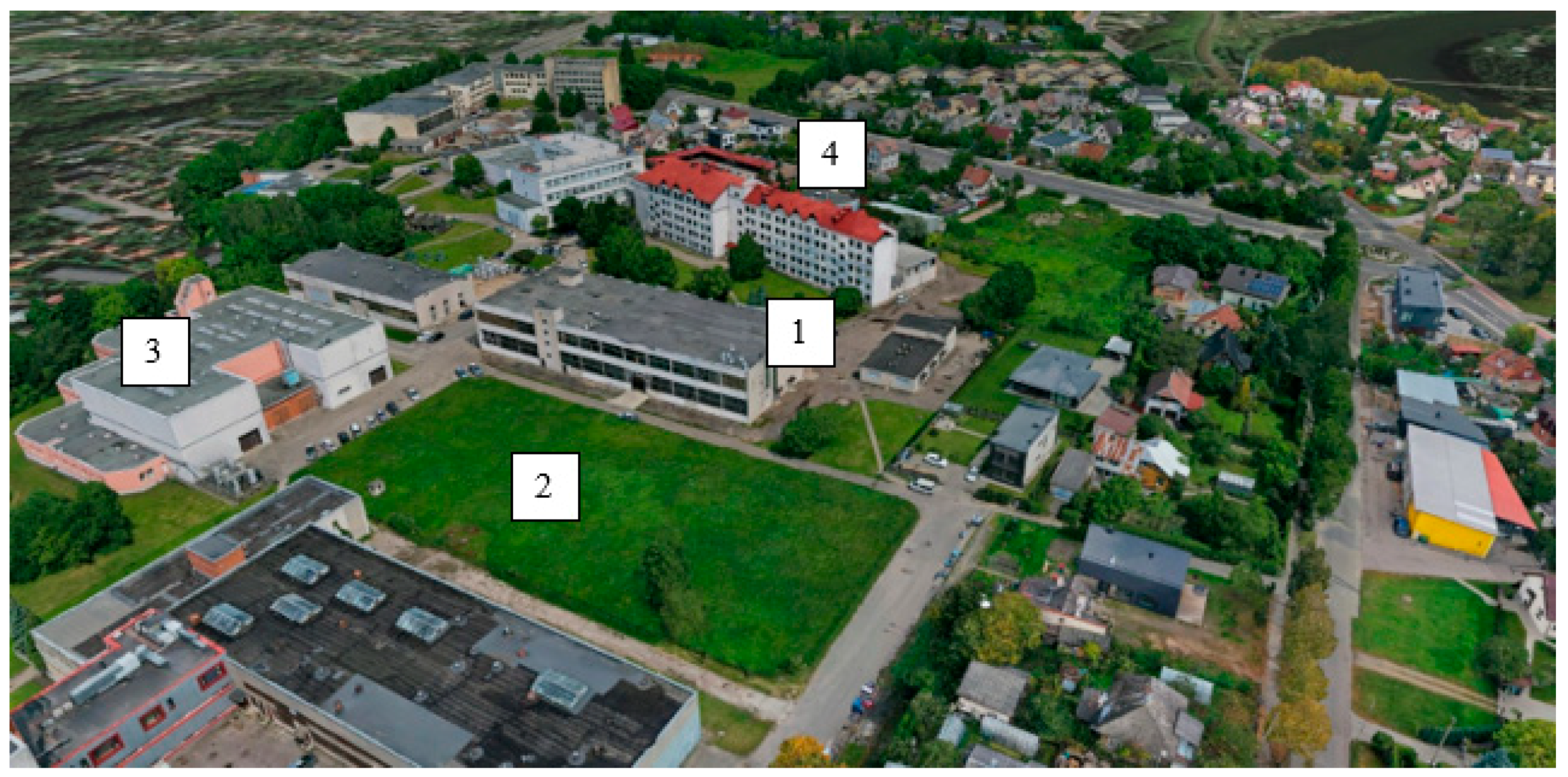
The PV installation was designed in four different structures: on the flat roof of building 1, on the ground level in field 2, vertically on building 3, and on the pitched roof of building 4 facing east and west sides (Figure 1).

These four locations represent common layouts for PV modules, i.e., modules placed on a flat roof (1), modules placed on the ground (2), modules placed vertically on a wall (3), and modules placed on a pitched roof (4), so the effect of shading could be examined in different scenarios. PV modules in the selected sites were mounted to make the best use of the available space for PV installation in the different structures. The size of each module array was dictated by obstacles and limitations present in that specific location.

2.4. Software and Data

The software “PV*SOL Premium 2020 (R1)” was used for the research in this paper. The program enables one to design and simulate the performance of the latest PV systems. This program estimates the potential power generation amount based on the geographical characteristics of the area (solar intensity, angle of drop of radiation, climate conditions, etc.), shading data (shading duration and loss of power due to casted shadows), and the optimal configuration of the PV system [42].

The software enabled the assessment of the possibilities for electricity generation via PV modules installed in different locations (on roofs, a wall, and the ground) of the analyzed site (Figure 1). The radiation profiles and climate data were retrieved automatically using the software from databases based on the specified geographic coordinates of the location [43]. In the analyzed case, data for Kaunas city are available for the period 1991–2010, as follows: the annual sum of global irradiation is 951 kWh/m², while the annual average temperature is 8.4 °C. Photovoltaic modules AS-M1449-H-400 with a nominal power of 0.4 kW manufactured by Allgemeine Elektricitäts-Gesellschaft (AEG) (Frankfurt, Germany) and SL-TL series inverters from model 2800 to 3600 T manufactured by SolaX Power Co., Ltd. (Hangzhou, China) were selected for analysis from the available list provided by the tool. The main information about the installed PV modules in different objects is presented in

Table 1. Information on the PV modules mounted on different objects.

Object	Total Installed Capacity (kW)	Number of Modules	Number of Inverters
Flat roof	130.4	326	37
Pitched roof	52	130	9
Wall	22.4	56	8
Ground	176	440	44
Total	380.8	952	98

.

The total installed capacity for each object was determined according to the number of modules installed in the available area. Other technical characteristics of the analyzed modules and inverters are presented in the datasheets [44,45].

Ambient 3D models were created with the Bentley ContextCapture Master program. The program generates photogrammetry from individual photos in a 3D terrain model to the coordinate system LKS 94 (EPSG:3346). The COLLADA (.dae) file format was selected for use in the “PV*SOL Premium 2020 (R1)” program [46].

2.5. Economic and Financial Parameters

One of the economic parameters used in this paper to determine the configuration of PV modules (in terms of optimal tilt angle and distance between PV rows) that yields the highest electricity generation was the levelized cost of electricity (LCOE). This indicator is calculated by dividing the total cost of a solar PP over its lifetime by the total amount of electricity generated by the solar PP over the same period:

$$\mathrm{LCOE}=TCost/TEl,$$

(1)

where LCOE is the levelized cost of electricity (EUR/kWh), TCost is the total cost of the solar PP over its lifetime (EUR), and Tel is the total amount of electricity generated by the solar PP over its lifetime (kWh).

The total cost of PV modules over the lifetime of the solar PP is given as the sum of two cost components—investment costs and operational costs—which can be expressed as

$$TCost={{\displaystyle \sum }}_{y=1}^{T}ICos{t}_y+{{\displaystyle \sum }}_{y=1}^{T}OCos{t}_y,$$

(2)

where ICost is the investment costs (EUR), OCost is the operational costs (EUR), y is the year, and T is the lifetime of the solar PP (years).

The investment cost depends on the total installed capacity of the PV modules and the relative investment cost per unit (e.g., kW) of the installed capacity:

$$ICos{t}_y=ICa{p}_y\cdot inv,$$

(3)

where ICap is the installed capacity (kW) and inv is the investment cost of the installed capacity per kW (EUR/kW).

The operational costs are based on the assumption that they cover a certain percentage of the initial investment cost of the solar PP:

$$OCos{t}_y=ICos{t}_y\cdot c/100,$$

(4)

where c is the operational costs as a percentage of the investment costs (%).

The total amount of electricity generated by the solar PP during its lifetime is evaluated as follows:

$$TEl={{\displaystyle \sum }}_{y=1}^{T}E{G}_y\cdot \left(1-d/100\right),$$

(5)

where EG is the amount of electricity generated by the PV modules each year (kWh) and d is the energy losses due to PV degradation each year (%). In the first year, d = 0.

One of the key indicators of an energy project’s economic viability is its payback period. To analyze the economic feasibility of a solar project, this methodology uses three financial indicators: payback period (PB), net present value (NPV), and internal rate of return (IRR).

The payback period refers to the length of time required to recoup the cost of the investment:

$$\mathrm{PB}=\frac{{{\displaystyle \sum }}_{y=1}^{T}ICos{t}_y}{{{\displaystyle \sum }}_{y=1}^T{C}_y},$$

(6)

where C_y is the net cash inflow in year y.

One of the drawbacks of the PB calculation method outlined in Formula (6) is that it does not take into account the time value of money. To address this issue, discounted payback period (DPB) and other financial indicators such as NPV and IRR can be used.

The DPB considers the time value of money by discounting the cash inflows of the solar PP:

$$\mathrm{DPB}=\frac{{{\displaystyle \sum }}_{y=1}^{T}ICos{t}_y}{{{\displaystyle \sum }}_{y=1}^T\frac{C_y}{{\left(1+r\right)}^y}},$$

(7)

where r is the discount rate (%).

The net present value quantifies the difference between the present value of cash inflows and outflows and is used to evaluate the profitability of a solar PP:

$$\mathrm{NPV}={{\displaystyle \sum }}_{y=1}^T\frac{C_y}{{\left(1+r\right)}^y}-{{\displaystyle \sum }}_{y=1}^{T}ICos{t}_y.$$

(8)

The internal rate of return is a discount rate that makes the NPV of all cash flows equal to zero and is also used to determine the profitability of potential investments in a solar PP:

$$0=\mathrm{NPV}={{\displaystyle \sum }}_{y=1}^T\frac{C_y}{{\left(1+\mathrm{IRR}\right)}^y}-{{\displaystyle \sum }}_{y=1}^{T}ICos{t}_y.$$

(9)

In other words, the IRR indicates the expected compound annual rate of return that will be earned on a solar PP.

3. Results

3.1. Analysis of Electricity Generation of PV Modules at Different Tilt Angles and Distances between PV Rows

The installation of PV modules at different tilt angles and distances between PV rows can greatly affect the amount of electricity generated. Technically feasible efforts (such as with proper roof construction) were made to select the optimal tilt angle and distance between PV rows when installing the PV modules. Buildings with flat roofs are particularly well-suited for this. In order to determine the optimal tilt angle and distance between PV rows for electricity generation in this case study, a comparison between different tilt angles and distances of PV modules was conducted based on the amounts of electricity generated per year. A building with a flat roof was chosen for the study, and a total of 12 combinations were considered: 4 tilt angle cases (0° (PV modules mounted horizontally), 15°, 30°, and 45°) and 3 distance between PV rows cases (1.00 m, 1.25 m, and 1.50 m). It is worth noting that in this case, the PV modules were installed with a direct south-facing orientation (azimuth 180°) rather than following the roof geometry.

To determine the combination of tilt angle and distance between PV rows that yields the best results in this case study, one of the indicators used for the comparison was the relative electricity generation per year (kWh), converted to one kilowatt (kW) of installed capacity. To compare the various cases in terms of economic performance, the levelized cost of electricity (LCOE) was calculated for each case. The methodology for calculating LCOE is outlined in Section 2.5, and key assumptions are discussed further. The analysis period (the lifetime of the solar PP) (parameter T) was considered to be 20 years. The investment costs per kW (parameter inv) were taken as 1000 EUR/kW. The operational costs per year (parameter c) were considered to be 2% of the investment costs. The annual power degradation due to physical depreciation (parameter d) was considered to be 1%. 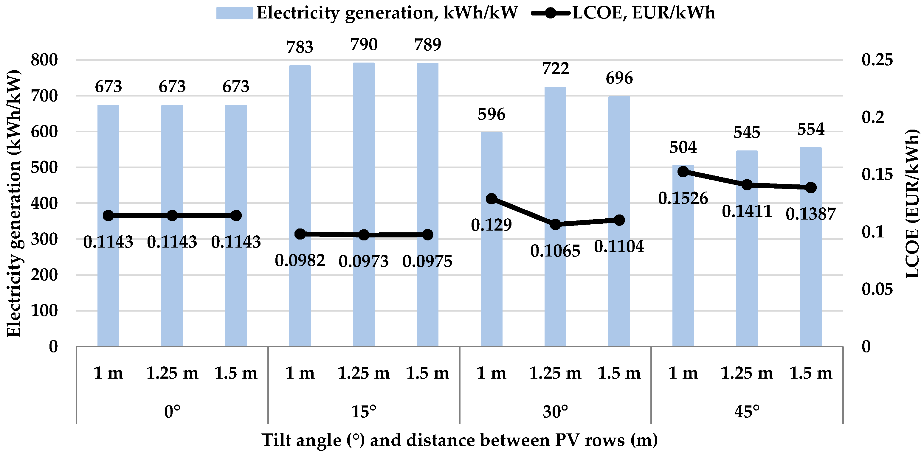These assumptions for the site being analyzed are based on information provided by the Applied Research Institute for Prospective Technologies [47]. 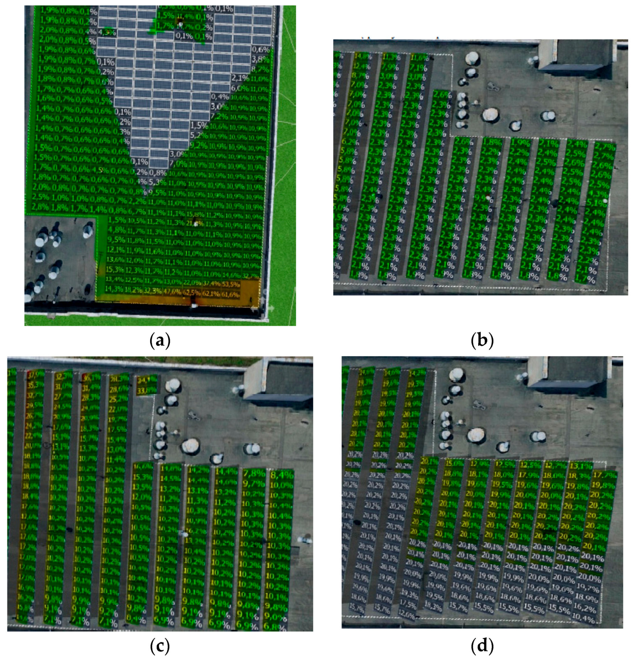The results of the relative electricity generation per year and LCOE for different tilt angles and distances between PV rows are presented in Figure 2. The visualization of shadow duration at various tilt angles can be found in Figure 3.

Figure 2 illustrates that the highest electricity generation (790 kWh/kW per year) would be achieved with PV modules that have a tilt angle of 15° and a distance of 1.25 m between PV rows in this case study. This combination of PV module installation also resulted in the lowest LCOE (0.0973 EUR/kWh) for all the cases analyzed. It is worth noting that these two parameters are strongly correlated. A negative correlation coefficient of 0.99 was observed, which indicates that higher relative electricity generation leads to a lower LCOE.

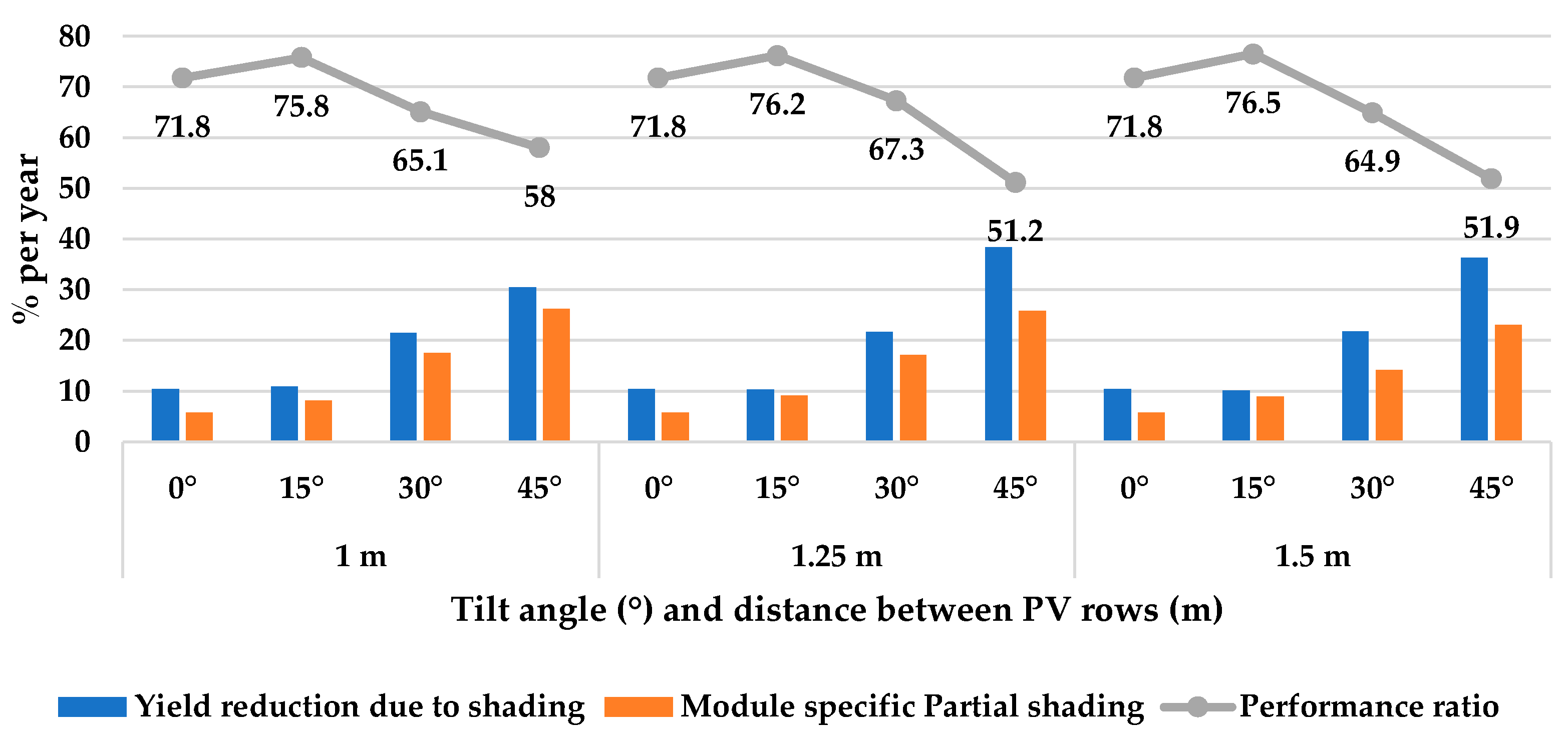
It was also observed that the main factor behind these results was the shadow that fell on the PV modules (as shown in Figure 3 and Figure 4). The yield reduction caused by both types of shading—shading due to surrounding objects and module-specific partial shading—was quite significant. As seen in Figure 4, the impact of shading when installing solar PV modules at tilt angles of 0° and 15° is similar, but the case with a 15° tilt angle is the most effective in terms of electricity generation because it has the highest performance ratio.

Cases with 30° and 45° tilt angles on this roof lost a significantly higher percentage of electricity generation due to shading compared with cases with 0° and 15° tilt angles. A similar conclusion is observed when comparing different distances between PV rows. A distance of 1.25 m resulted in the lowest shading and highest performance ratios among the analyzed cases. The highest level of shading was primarily caused by module-specific partial shading, which is formed mainly due to shadows of PV modules falling on other PV modules in different rows. This also affects the performance ratio of PV modules, and it decreases as the tilt angle increases.

The optimal tilt angle obtained in this study differs from those found in other studies analyzed for the same location. The main reason for these differences is that this study includes shading effects in the analysis, which changes the output for the optimal parameters of PV module arrays. When shading has not been taken into account, other studies and sources have reported tilt angles of 33° [5] and 39° [8,9] for the same location. However, the presented study shows that the highest performance ratio is observed at a tilt angle of 15° when shading is taken into account. Therefore, in this case study, for a flat roof and on the ground, a tilt angle of 15° and a distance of 1.25 m between PV rows were selected for further analysis.

3.2. Analysis of Electricity Generation of PV Modules Installed on Different Types of Objects

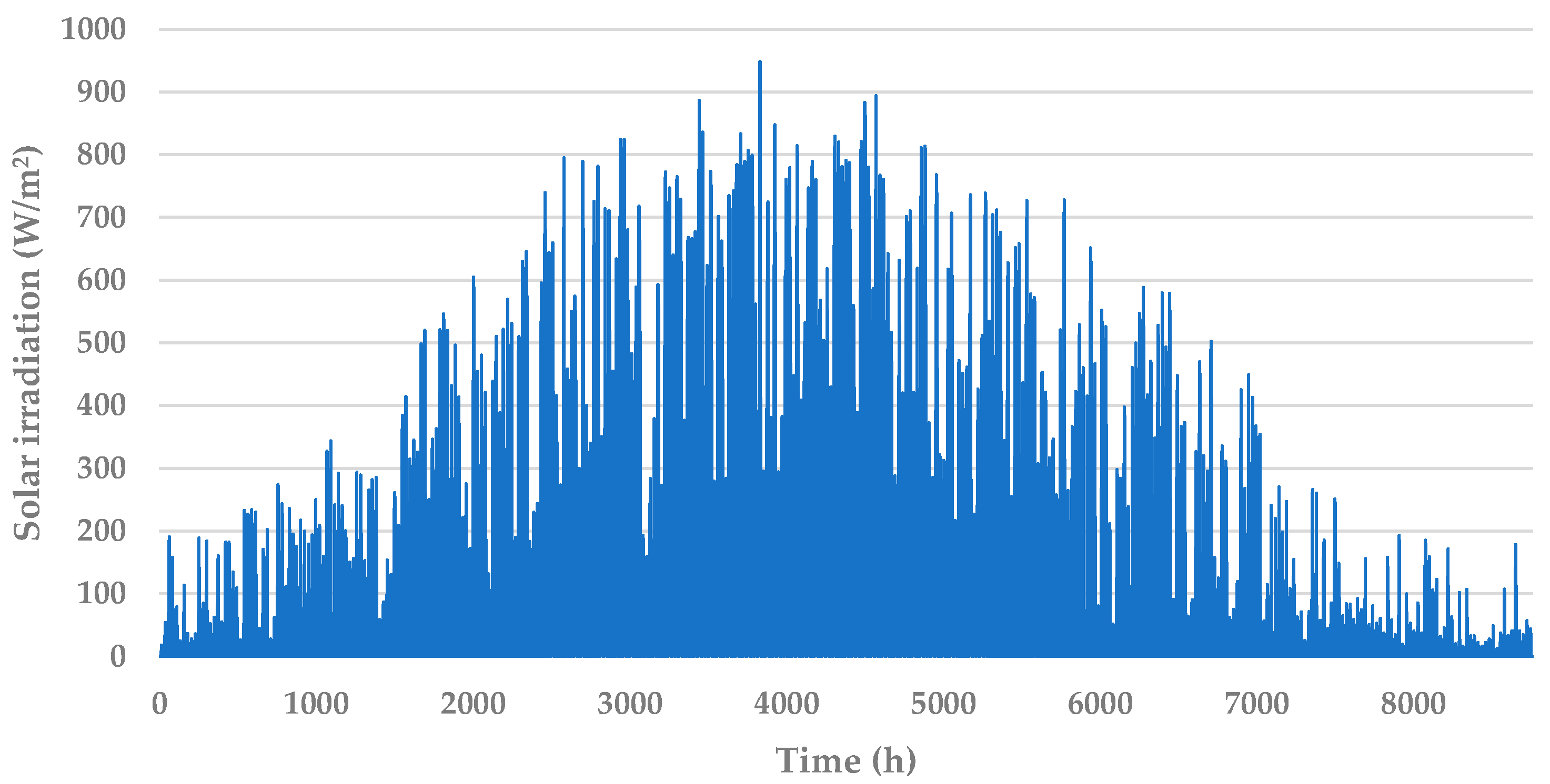
Electricity generation in solar PPs is heavily influenced by the intensity of solar radiation, climatic conditions, and installed capacity. The latter parameter is highly dependent on the technical characteristics of buildings; thus, arrays of PV modules are designed to optimize the use of the roof or wall area of buildings. Since the results of electricity generation in solar PPs are heavily dependent on the intensity of solar radiation, hourly data for one year for Kaunas conditions are presented in Figure 5.

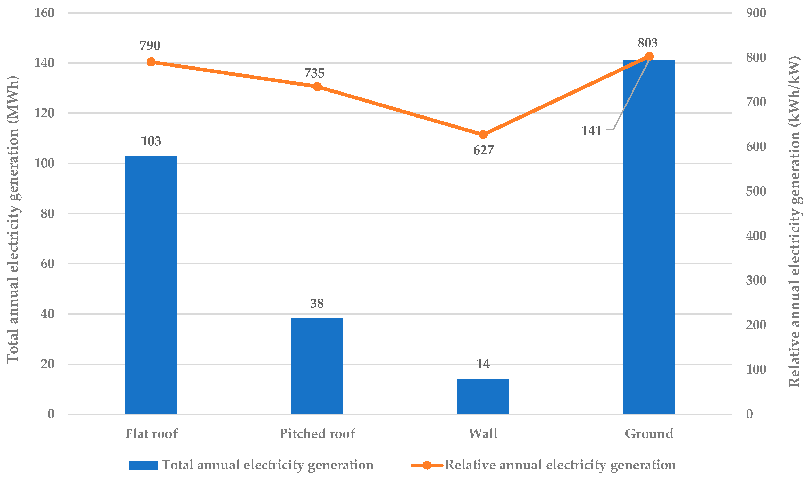
Modeling of the electricity generation from various solar PPs using the “PV*SOL Premium” tool was carried out on an hourly basis for one year. Figure 6 illustrates the total (MWh) and relative (kWh/kW) annual electricity generation from PV modules for each object.

The total generation amounts directly depended on the installed capacity of the PV modules, which varied greatly among the analyzed objects, as presented in Table 1. The indicator of relative annual electricity generation, which is recalculated to one kW of installed capacity, is more suitable for comparing different objects. In this case study, the best results were demonstrated by PV modules mounted on the ground and flat roof, as they were most suitable for installation with an optimal tilt angle of 15°. PV modules mounted on the wall demonstrated a relatively lower rate of electricity generation, possibly due to the steep tilt angle of the modules. However, when comparing the relative annual electricity generation, the differences between the analyzed objects were not substantial and can be explained by the shading profiles of the environment.

As the results indicate, the intensity of solar radiation and the installed capacity of the solar PP are important factors, but electricity generation is also affected by other factors, such as the environment or the location of PV modules, which may be influenced by shadows cast by adjacent structures.

Table 2. Comparison of shading influence and performance between the analyzed objects.

Object	Yield Reduction Due to Shading (%)	Module-Specific Partial Shading (%)	Performance Ratio (%)
Flat roof	10.3	9.15	76.2
Pitched roof	1.4	0.76	81.1
Wall	0	0	82.1
Ground	9.7	5.95	79.4

demonstrates that shadows had the greatest impact on the solar PP mounted on the flat roof, resulting in a 10.3% reduction in yield due to shading per year. However, a majority of this shading was caused by module-specific partial shading, which was also the highest (9.15%) among the analyzed installations of PV modules.

The impact of shadows is also evident in the performance ratios of the PV modules: the less shading on the PV modules, the higher their performance is observed to be.

3.3. Result Comparison with the PVGIS Tool

To illustrate the effect of shading on PV energy output, simulated results were compared with results of the PV system with no influence of shadows. The PVGIS tool [8] was employed to simulate the performance of the PV system.

The PV system on the flat roof with a 130.4 kW installed capacity, a tilt angle of 15°, and a distance of 1.25 m between PV rows, which demonstrated the highest relative annual electricity generation of building roofs (Figure 6), was selected for a comparison analysis with PVGIS simulations. The simulated results for the flat roof were discussed in Section 3.1 and Section 3.2 In PVGIS simulations, two cases were simulated: a 15° tilt angle (the same as in the simulation with shading) and an optimal tilt angle optimized via PVGIS. The assumptions used in the PVGIS simulations were aligned as much as possible with the assumptions used in the simulation with shading.

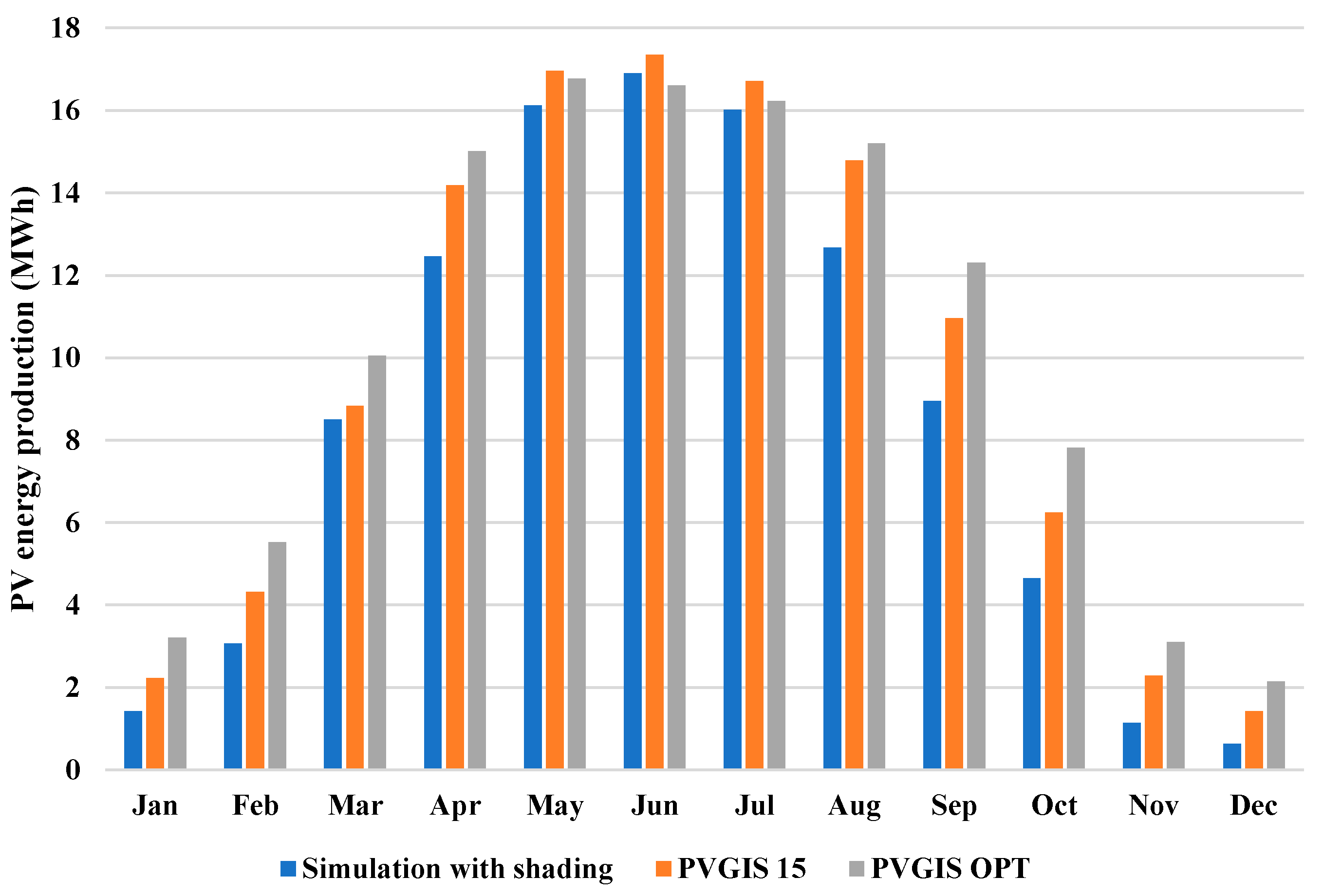
Figure 7 illustrates the annual PV energy output for the simulated case with the influence of shading, which represents our proposed method, and two PVGIS simulations with no influence of shading.

The variable Simulation with shading represents our analyzed case, while the variable PVGIS 15 refers to the PVGIS simulation with a 15° tilt angle, and the variable PVGIS OPT represents the case of the optimal tilt angle selected by the PVGIS tool, which is 39° in this simulation. Both PVGIS simulations did not consider the shading effect of the analyzed object. The results demonstrate that PV modules with a lower tilt angle provide a higher energy output during summer months, while PV modules with a higher tilt angle perform better during winter months. However, when the shading on PV modules is taken into account, the total PV energy production is significantly lower.

When comparing relative electricity generation per year, the simulation with shading was observed as producing 790 kWh/kW, while the PVGIS simulation with a 15° tilt angle yielded 892 kWh/kW, and the simulation with a 39° tilt angle yielded 951 kWh/kW. The results of the PVGIS simulations show a difference of 11.42% (for the 15° tilt angle) and 16.93% (for the 39° tilt angle) when compared with the simulated case with shading, which is significant.

The comparison between the simulated case with shading effects and the PVGIS simulations demonstrates that our proposed method enables an 11.42% more accurate estimation when the same tilt angle is considered. The obtained results confirm those presented in Table 2, wherein a yield reduction of 10.3% due to shading was obtained for the flat roof.

3.4. Comparative Analysis of Electricity Generation of PV Modules and Actual Electricity Consumption

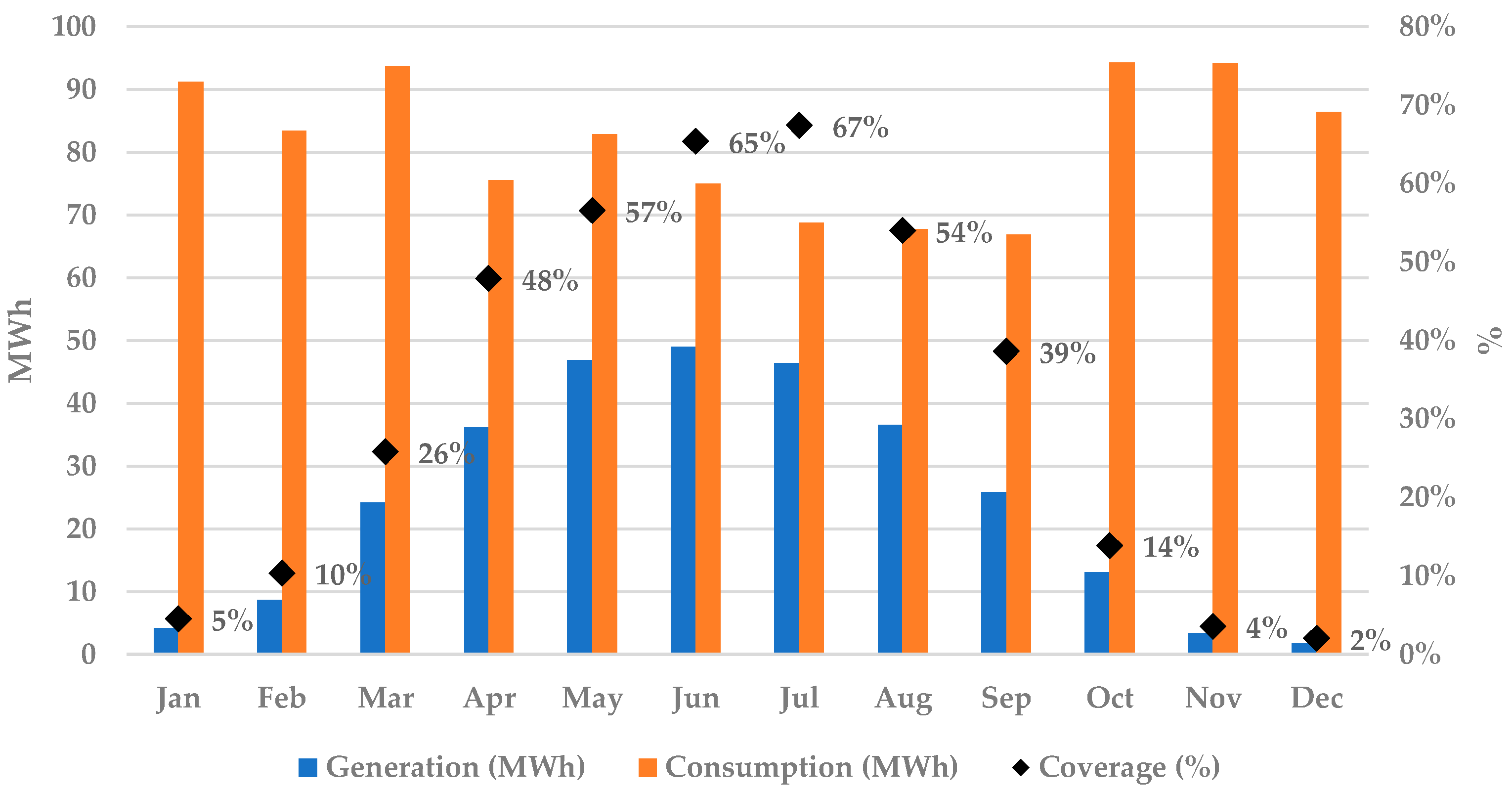
Another task of this study is to determine how much of the consumer’s total electricity consumption could be met or covered by electricity generated by PV modules installed in the analyzed site. The electricity consumption data used in this comparison were collected from the analyzed buildings in the PV installation, i.e., building 1, building 3, and building 4 (Figure 1). A comparative analysis between the monthly electricity generation by the PV modules and the actual electricity consumption, as well as the percentage, which shows what part of consumption is covered by generation in each month, is presented in Figure 8.

The majority of electricity consumption would be covered by electricity generated from PV modules from May to August, covering an average of 61% of the electricity demand. The lowest difference between electricity consumption and generation is in July when generation covers 67% of the electricity consumption for that month (Figure 8). This is due to one of the lowest electricity consumptions per month compared with other months, and the second largest (after June) level of electricity generation by PV modules in that month. In the winter months, electricity generation from solar PPs would be able to cover only from 2% in December and up to 10% in February of that month’s electricity consumption.

3.5. Economic and Financial Analysis

In order to evaluate the economic and financial performance of installed PV modules, it is necessary to calculate the potential savings from generating electricity with PV modules instead of purchasing electricity from a supplier. This largely depends on the net metering payment method chosen by the prosumer and the applicable electricity tariffs for consumers purchasing electricity from the supplier.

In Lithuania, four net metering methods are proposed by the energy distribution operator, and tariffs for the electricity storage service are set once a year by the National Energy Regulatory Council. In this study, the following net metering payment methods for prosumers at low voltage (0.4 kV) in 2020 were used:

• Method 1. Fixed payment for stored and recovered electricity at 0.05203 EUR/kWh.
• Method 2. Fixed payment for the installed PV capacity at 2.6378 EUR/kW/month.
• Method 3. A mixed method of payment for stored and recovered electricity at 0.02662 EUR/kWh and payment for the installed PV capacity at 1.3189 EUR/kW/month.
• Method 4. Payment in kWh by percentage. The prosumer recovers 64% of the stored electricity. A total of 36% of the prosumer’s generated electricity is used by the energy distribution operator.

Additionally, the electricity tariff of the “Standard” plan proposed by the electricity supplier, which is 0.137 EUR/kWh for low voltage and has been in force since 1 July 2020, was used in this study. It should be underlined that these tariffs and payment methods are constantly reviewed and updated.

In 2022, energy prices, including electricity, drastically increased due to global reasons such as limited supplies, increased demand, a shortage of reserves, the war in Ukraine, and others. However, these prices can be considered inconsistent with the real situation in the energy sector and were caused in the face of a war situation, panic, and crisis. Therefore, it was decided not to take the 2022 situation into account in this study as it may distort the actual results, but to use the stable energy prices that prevailed in 2020.

It was noted that the most attractive payment method for a prosumer is highly dependent on the proportion of electricity that is consumed simultaneously during generation. If the amount of electricity generated by PV modules is greater than the amount of consumed electricity, the excess is fed into the electricity grid. In the analyzed case, 83% of electricity per year would be consumed simultaneously during generation, while the remaining 17% would be fed into the grid for storage. This result influences the optimal choice of the prosumer’s payment method.

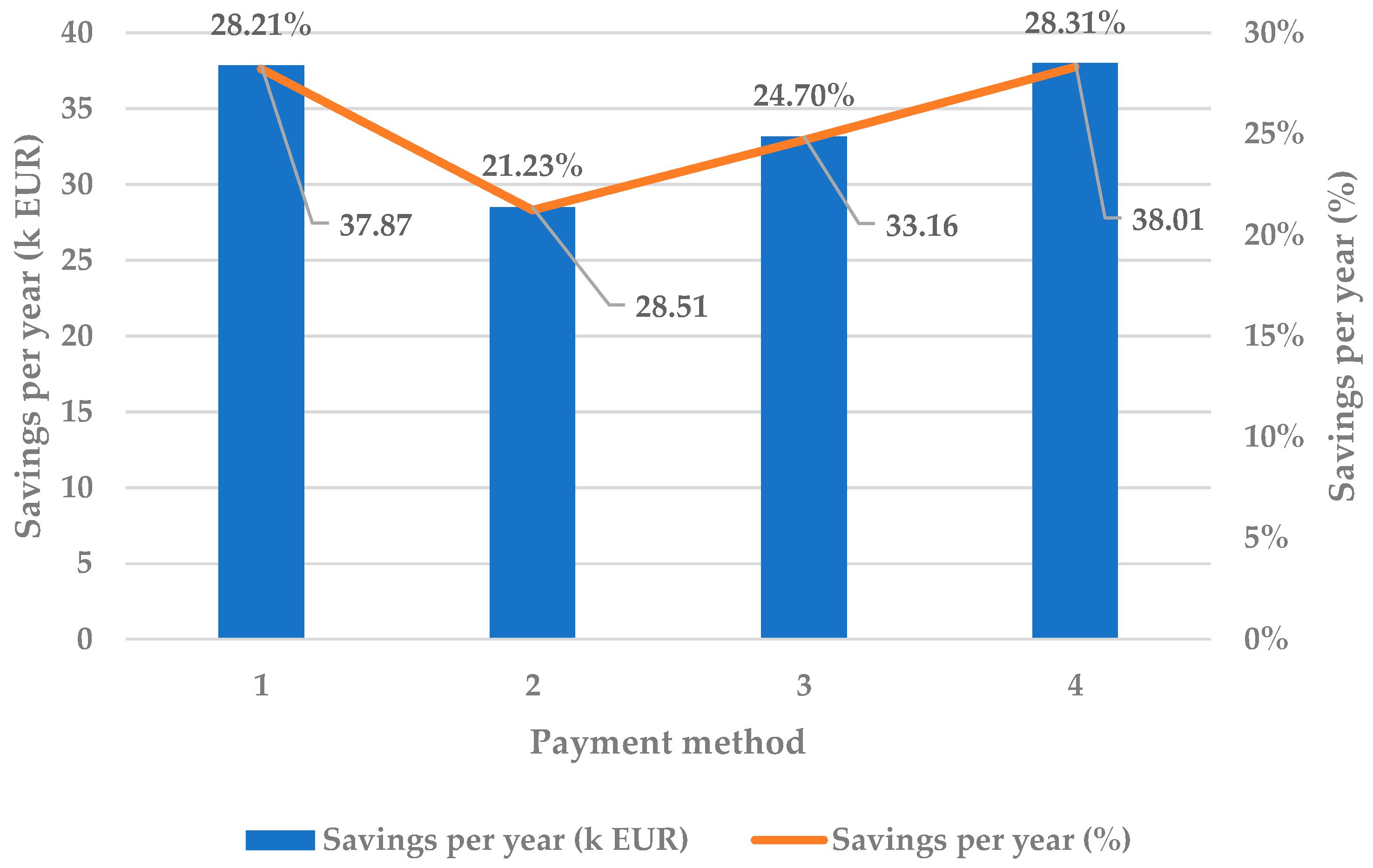
For a period of one year, potential savings were modeled for each of the four net metering payment methods. Figure 9 demonstrates that the highest savings would be achieved by choosing payment methods 1 or 4, with savings of 28.21% and 28.31% per year, respectively.

When analyzing these indicators for the annual base, it was determined that electricity generation in the installed PV modules in the analyzed site objects would cover a total of 30.3% of the annual electricity consumption per year.

The main reason for the attractiveness of these two methods is that they are based on the kWh of electricity supplied to the grid and subsequently recovered (method 1) and the payment in kWh, where 36% of the electricity supplied to the grid is left to the network operator (method 4).

In order to evaluate the economic attractiveness of the analyzed solar PP, three financial parameters that were described in Section 2.5 were considered: payback period, net present value, and internal rate of return. The results of these indicators highly depend on the payment method selected and whether government support is considered for the analyzed solar PP. As a result, these 3 indicators were evaluated for each payment method in 4 scenarios of government support (0%, 30%, 50%, and 80%).

A financial analysis of the installed PV modules was performed considering the potential amount of generated electricity, energy and cost savings, investment and operating costs, and other related parameters during the lifetime of the solar PP. As the results highly depend on the values for these parameters, the key assumptions for the calculations were already introduced in Section 2.4 and Section 3.1, and additional assumptions are given in

Table 3. Key assumptions for the economic and financial analysis.

Discount Rate	Total Installed Capacity	Savings Per Year		Government Support
5%	380.8 kW	Method 1	37.87 k EUR	Scenario 1	0% (no support)
		Method 2	28.51 k EUR	Scenario 2	30%
		Method 3	33.16 k EUR	Scenario 3	50%
		Method 4	38.01 k EUR	Scenario 4	80%

.

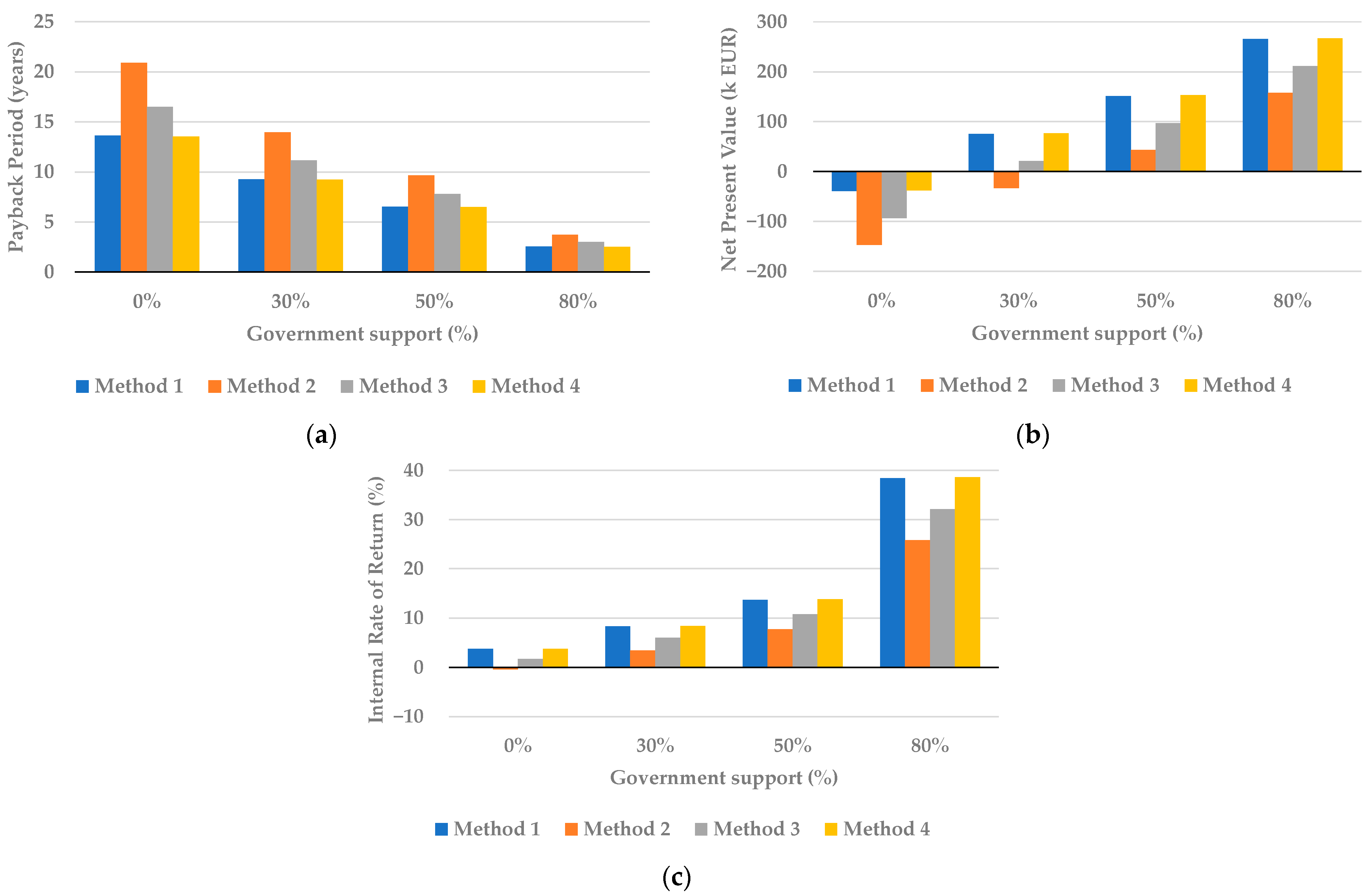
The results reveal that payment methods 1 and 4 show practically identical results for the financial indicators due to very similar savings; therefore, they will be further treated as demonstrating the same results. As shown in Figure 10a, the PB of the solar PP decreases as the intensity of government support increases. With 30% support, methods 1 and 4 already have a PB of less than 10 years, while method 2 achieves such a PB only with 50% support. With 80% support, the PB for the analyzed payment methods ranges from 2.5 to 3.7 years.

The NPV analysis (Figure 10b) demonstrates that the results also highly depend on the payment method chosen and government support. A positive NPV for payment methods 1, 3, and 4 is reached with 30% support, while method 2 requires a 50% funding intensity for the NPV to reach a positive value. Although 50% support gives a positive value in all analyzed payment methods, the absolute value of NPV is quite different and ranges from 43 k to 153 k EUR. With 80% support, the NPV reaches approximately 265 k EUR when payment method 1 or 4 is selected.

The results of the IRR analysis (Figure 10c) highly correlate with the NPV values when the highest profitability of the analyzed solar PP is achieved for payment methods 1 and 4. An IRR over 5% (the desired discount rate) is observed in the scenario with 30% government support for methods 1, 3, and 4, while for method 2, 50% support is required to achieve an IRR of at least 5%. At a funding intensity of 80%, the IRR for all analyzed payment methods increases significantly and varies from 26% to 39%.

In summary, the results of the economic and financial analysis in this case study indicate that if the prosumer chooses the most attractive payment methods 1 or 4 for the storage service, at least 30% of government support would be required for the solar PP to be profitable. However, if payment method 2 is chosen, the intensity of funding support should be at least 50% to make the project profitable.

4. Conclusions

In this paper, a digital environment produced using UAV-based photogrammetry was used to evaluate the site’s potential to produce electricity from solar energy considering shading effects. During the research, the following observations were made:

• Photogrammetry created an accurate 3D model of the site, which depicted structures, vegetation, and other small objects that can cast shadows and create obstacles for arrays of PV modules.
• Although the installation of PV modules at a steep tilt angle makes more efficient use of solar radiation, the amount of electricity produced by PV modules may decrease due to specific module shadows. In the analyzed case, the optimal tilt angle for PV modules on flat surfaces was found to be 15° (the analyzed variants were 0°, 15°, 30°, and 45°) with a distance of 1.25 m between PV rows. In this configuration, the relative electricity generation was 790 kWh/kW, which is significantly lower compared with a case without shading on PV modules.
• The comparison of simulations of our proposed method, which considers the shading effect, with the simulations of the tool that does not consider shading showed that our proposed method enables an 11.42% more accurate estimation due to the inclusion of shading influence.
• The biggest loss in electricity production were observed on flat surfaces such as the ground and a flat roof. On these surfaces, shading caused reductions in yield of 10.3% and 9.7%, respectively, and module-specific partial shading was responsible for losses of 9.15% and 5.95%, respectively.
• A comparative analysis of the potential electricity generation from solar PPs and actual electricity consumption by the prosumer showed that electricity production from PV modules in the research location (Kaunas, Lithuania) can cover up to 30.3% of the annual prosumer electricity demand. In July, when electricity production peaks, it manages to cover up to 61% of the prosumer’s demand. At the low point of production, during December, only 2% of electricity demand is covered.
• The attractiveness of the payment method for the prosumer for stored and recovered electricity service greatly depends on the amount of electricity consumed simultaneously during generation from the solar PP. In the analyzed case, it was observed that 83% of the electricity generated during the year would be consumed simultaneously, with the remaining 17% being fed into the grid for storage.
• For a period of 1 year, the highest potential savings would be achieved by choosing the first or fourth prosumer payment method, with savings of 28.21% and 28.31%, respectively.
• The financial analysis of the solar PP deployment project revealed that without external financial support, the project is not economically viable. This is evidenced by a relatively long payback period ranging from 13 to 21 years, a negative net present value between −38 k and −147 k euros, and the internal rate of return not exceeding the required discount rate of 5%. Moreover, if the prosumer chooses the most attractive first or fourth payment method for the storage service, at least 30% of external financing support is necessary for the solar PP to be profitable.
• This study demonstrated that the feasibility of a solar PP project is greatly dependent on the characteristics of the building (roof structure, facade shape, south-facing, etc.), the prosumer’s electricity consumption load schedule, the chosen payment method for storage and recovery of electricity, and the availability of external funding. Furthermore, PV-generated energy can enhance energy security by adding diversity to the overall electricity generation mix.