
Statistical Optimization of E-Scooter Micro-Mobility Utilization in Postal Service


Directorate for Strategy Development, Ministry of Transport and Infrastructure, Ankara 06338, Turkey
Energies 2023, 16(3), 1291; https://doi.org/10.3390/en16031291
Submission received: 19 December 2022
/
Revised: 16 January 2023
/
Accepted: 17 January 2023
/
Published: 25 January 2023
(This article belongs to the Topic Electromobility and New Mobility Solutions in Sustainable Urban Transport Systems)
(This article belongs to the Section E: Electric Vehicles)
(This article belongs to the Section E: Electric Vehicles)
Abstract
:New-generation technologies on vehicles provide many advantages in terms of cost, time, and the environment in the transportation, logistics, freight, and delivery service sectors. This study aimed to measure the effect of using e-scooter vehicles in mail delivery on the energy cost and delivery time in Turkey. Considering the number of test drives in e-scooter applications of potential regions, the amount of energy consumption and driving time data were used. The number of test drives for each e-scooter was assumed as a package or postal delivery amount. The methodology of this study consisted of measuring the effect of input parameters on output variables using the linear response optimization regression method and minimizing the amount of energy consumed and delivery time. The nine input variables and two output variables based on the test drive were analyzed in this study. The distance to the delivery address, region where the delivery address was located, and temperature were found to be statistically significant predictors of the amount of energy required for delivery. The statistical significance levels of time zone, distance, temperature, rainfall, and region factors were calculated as 0.053, 0.001, 0.0033, 0.044, and 0.042, respectively. Driver age, data time zone, distance, wind speed, and delivery region factors affected the time required for delivery with an e-scooter. The statistical significance levels of these factors were calculated as 0.02, 0.001, 0.001, 0.043, and 0.001, respectively. Additionally, N (p; 0.042), NE (p; 0.030), and W (p; 0.057) wind directions directly influenced the delivery time. SE (p; 0.017) was the only wind direction that statistically significantly affected energy consumption. The objective functions were estimated by calculating the optimum values of the input parameters for the minimum energy consumption and delivery time. The optimum values of both input and output variables were calculated based on the desirability values of the optimization models, which were in the optimum solution set. The average data of the optimum values of the objective functions were computed as 2.83 for the number of tests and TRY 0.021 (per 0.098 km) for the energy cost required for delivery. The necessity of using e-scooters, which are more environmentally friendly, economical, and time-saving than traditional delivery vehicles, in postal delivery service is among the prominent suggestions of this study.
1. Introduction
The growth of the urban population and the increase in e-commerce activities affect the complexity of package or mail delivery processes [1]. Factors such as complex construction, population density in cosmopolitan cities [2], rapid communication, and technological developments keep the package or mail delivery service sector alive [3]. The postal delivery industry is developing to provide customers with a faster and higher quality service. The postal delivery industry must overcome many obstacles to respond instantly to its customers [4]. These obstacles include many parameters such as energy, cost, environmental factors, and complex delivery networks [5].
Today, the postal transportation sector has two significant problems: energy [6] and time [2,7]. The energy costs needed during the delivery period of the vehicles used in the postal delivery sector are increasing daily [8]. Most traditional delivery vehicles are powered with gasoline (diesel or oil) [9]. The traditional vehicle fleets of the postal delivery sector consist of vehicles that consume gasoline or diesel, such as minivans, buses, trucks, pickup trucks, combi vans, motorcycles, and automobiles. This sector is turning to different delivery vehicles to overcome energy costs. The number and types of vehicles that use electricity to meet energy needs are increasing daily. The postal delivery sector also wants to benefit from these means of transportation that provide positive advantages [10]. For this reason, it will not be surprising for customers that electric vehicles, which reduce energy costs, are preferred for mail delivery.
Following the emergence of shared e-scooters among the opportunities offered by the new generation of technology and micro-mobility vehicles, participation in their use is increasing. These vehicles, primarily preferred for daily and short-distance travel, have started to be used for different purposes over time. E-scooter vehicles, among the micro-mobility vehicles for daily travel, are heavily preferred in different parts of the world. A study reported that approximately 2.5 billion trips were made in 2018 with e-scooter vehicles for travel in New York City, USA [11]. As a similar finding, another study examined more than 425,000 trips in Indianapolis City, USA, emphasizing the increasing demand for e-scooter vehicles [12]. Dias et al. claimed that more than 400,000 drivers in Spain make more than 1.5 million trips in a year with shared e-scooter vehicles across the country [13]. In the same study, the researchers found that more than 1.8 million trips are made in a year in Lisbon, Portugal, where drivers prefer e-scooter vehicles for daily travel [13]. Although the use of shared e-scooters also significantly impacts the e-scooter industry, it has been mentioned that there are 85,000 shared e-scooters in more than 100 cities in the USA [14]. Another study contributed to keeping the e-scooter industry alive by emphasizing that shared e-scooter vehicles will operate in approximately 60 cities in Germany until 2021 [15].
Other reasons why drivers prefer e-scooter vehicles are related to driver behaviors and are due to reasons such as difficulty in accessing other vehicles and parking problems. One study reviewed 417 articles and investigated the psychosocial characteristics of e-scooter drivers, focusing on behavioral and risk-related aspects [16]. Another study emphasized that the usage rate increased with e-scooter corrals by sharing e-scooter usage and driver perceptions [17]. Another reason why e-scooter vehicles are preferred is that the vast majority of drivers think that these vehicles are economical and environmentally friendly [18]. Considering all these factors, the use of e-scooters is increasing exponentially in different parts of the world. As a result, it is not surprising that the use of shared and rentable e-scooter vehicles among micro-mobility vehicles, especially for daily trips, is widespread worldwide. Still, these vehicles significantly contribute to their users in terms of time, energy, and cost.
Many studies that revealed the difference between traditional and electric vehicles in terms of energy costs have been discussed. A significant portion of the costs (insurance, maintenance, personnel, etc.) incurred during postal or package delivery is due to energy costs. Trucks and derivative vehicles used in the package or mail industry account for 23% of the energy used for transportation [19,20]. A study predicted that the preferred micro-mobility vehicles for transport can reduce energy consumption by 1% at the national level and 2.6% at the city-center level, and that with the widespread use of micro-mobility there will be significant decreases in the amount of energy required for transportation [21]. With the use of e-scooter vehicles in transportation or logistics, approximately 65% of the operating costs are calculated as energy costs [22]. The cost of the amount of energy required for these vehicles also varies depending on the type and size of the material used for the battery, and approximately 15% can be saved. In one study, Nocerino et al. reported that in trials with electric micro-mobility vehicles, they achieved energy savings of between EUR 0.036 and EUR 0.194 per km. These savings were calculated as the maximum daily energy cost of EUR 11 for each e-vehicle [23]. Many studies have emphasized in detail that with the widespread use of micro-mobility vehicles in transportation or logistics (for specific package sizes and weights), significant savings in energy costs are achieved. This study emphasized that using packages with a particular weight and height to deliver to customers with e-scooter vehicles provides substantial energy cost savings for the Turkish postal service unit.
In addition to the positive contribution of electric vehicle use to the energy cost, electric energy-powered delivery vehicles also provide positive impacts on environmental parameters. A study revealed that electric tricycles are a more viable alternative from economic, ecological, and social aspects [1]. One study suggested that traditional delivery vehicles used for mail or package delivery have too much impact on CO2 emissions. Some studies shared some statistical results that road transport increases CO2 emissions [24]. Trucks and derivative vehicles used in the package or mail transport system are responsible for 24% of greenhouse gas emissions [19,20]. As the size of the vehicles used for transportation and the distance of the delivery area increases, the environmental impacts of those vehicles become increasingly negative. A study has shown that air transport is approximately four times more carbon-intensive than truck transport and approximately ten times more carbon-intensive than rail transport [25]. Preferring vehicles such as electrically powered e-scooters for package or mail delivery has positive environmental impacts. One study emphasized that using an e-scooter vehicle throughout its operating life cycle decreased emissions to 57 g CO2 eq./km [26]. Another study noted that e-scooters used in transportation (excluding the logistics sector) minimized CO2 emissions, energy costs, traffic volume, and congestion [27].
Especially in cosmopolitan cities, with the proliferation of complex settlements and the complexity of road routes, negative results occur in the delivery times of mail or packages with traditional vehicles [28]. Traditional logistics vehicles used for mail or package delivery cause 8–10% of congestion in urban traffic flow [29]. However, the preference for micro-mobility cars in the transportation and logistics sector reduces the utilization rate of road capacities by 30% [30]. A study has emphasized that the time required for a postal or package delivery is shorter in vehicles powered by electrical energy in micro-mobility vehicles than in traditional vehicles [23]. Micro-mobility vehicles, such as e-scooters, are not seriously affected by factors such as morning and evening traffic jams, weather conditions, and road working conditions in postal or package delivery time zones, unlike traditional delivery vehicles [31]. Lia et al. compared the capacity with the driver’s weight (kg), traffic speed (km/h), amount of emissions, range of usage (km), and transportation costs for cargo bikes (170–210, 20, zero, 50–70, and low, respectively), e-cargo bikes (1710–200, 20, low, 50–70, and high, respectively), e-scooters (180–250, 25, low, 50–120, and average, respectively), and vans (710–1490, 8–15, high, not applicable, and very high, respectively), which are all vehicles used in the transportation and logistics sectors [31].
Researchers have presented different methods to measure the impact of e-scooter vehicles on cost, energy, and the environment. Hosseinzadeh et al. used a spatial analysis approach to measure the impact of demographics, density, diversity, design, urbanism scores, public transport distance, and transportation-related factors on e-scooter trips [32]. Another study proposed a proper and effective procedure for designing a reluctance machine using a multi-objective optimization technique by working on the battery specifications of e-scooter vehicles [33]. Another study investigated the factors affecting charging station locations using a new Pythagorean fuzzy multi-criteria decision-making methodology for e-scooter location selection [34]. Ciociola et al. created a simulation approach that used open-access data to develop a demand model that supports and generalizes e-scooter vehicles in a center [35]. Another article described an optimization model that will minimize the cost of owning an electric micro-mobility by working on using electric micro-mobility vehicles in transportation and working on energy-generating batteries [36]. Most studies on e-scooter vehicles have used statistical methods to analyze environmental factors. Hollingsworth et al. used statistical methods to measure the effects of environmental loads associated with charging e-scooters on material and production loads of e-scooters and transporting scooters to overnight charging stations [37]. Another study analyzed e-scooter riding in Austin and Minneapolis using GIS (geographic information system) hotspot spatial analysis and negative binomial regression models to analyze environmental factors [38]. This study used a linear response optimization regression model to measure the effect of nine independent variables on energy costs and delivery times of e-scooter vehicles used for mail and package delivery. The statistical analyses were made, and the magnitude of the effect of the input variables on the output variables and the results (positive or negative) were analyzed in this study.
The novelty of this research emphasizes the necessity of using electric micro-mobility vehicles with the possibilities offered by the new generation technology, unlike the traditional delivery vehicles used in the postal service sector. One of the essential features that distinguish this study from other studies is that this study used a statistical optimization model developed in terms of cost, time, and environmental factors, suggesting that e-scooter vehicles, which are generally preferred for travel, should be used for mail or package delivery. Another feature is that a wide range of data belonging to more than one region were selected to verify the validity of the optimum and statistical values. In addition, this study has revealed a useful model by emphasizing that micro-mobility tools, such as e-scooters, should be used for different purposes.
This study consists of five main parts. In the literature review the cost, energy, and environmental effects of traditional delivery vehicles used for mail or package delivery and electric vehicles, such as e-scooters, are discussed. The rest of the paper is structured as follows. Detailed information about the method developed for the recognition and processing of actual data used in this study is given in the second section. The numerical results of the study are discussed in the third section. The effects of the numerical results obtained with the developed method are mentioned in the study’s Discussion. The technique used in this study to contribute to other studies, the results, and comments are discussed in the last part of the study.
2. Materials and Methods
This study focused on the necessity of e-scooter applications by calculating the optimum values of input and output parameters using data from 6213 e-scooter drivers (the original data) [39]. The methodology of the study adopted a linear response regression optimization method to measure the effects of the input parameters on the output variables and to obtain the optimum values of the variables.
2.1. Data Compilation
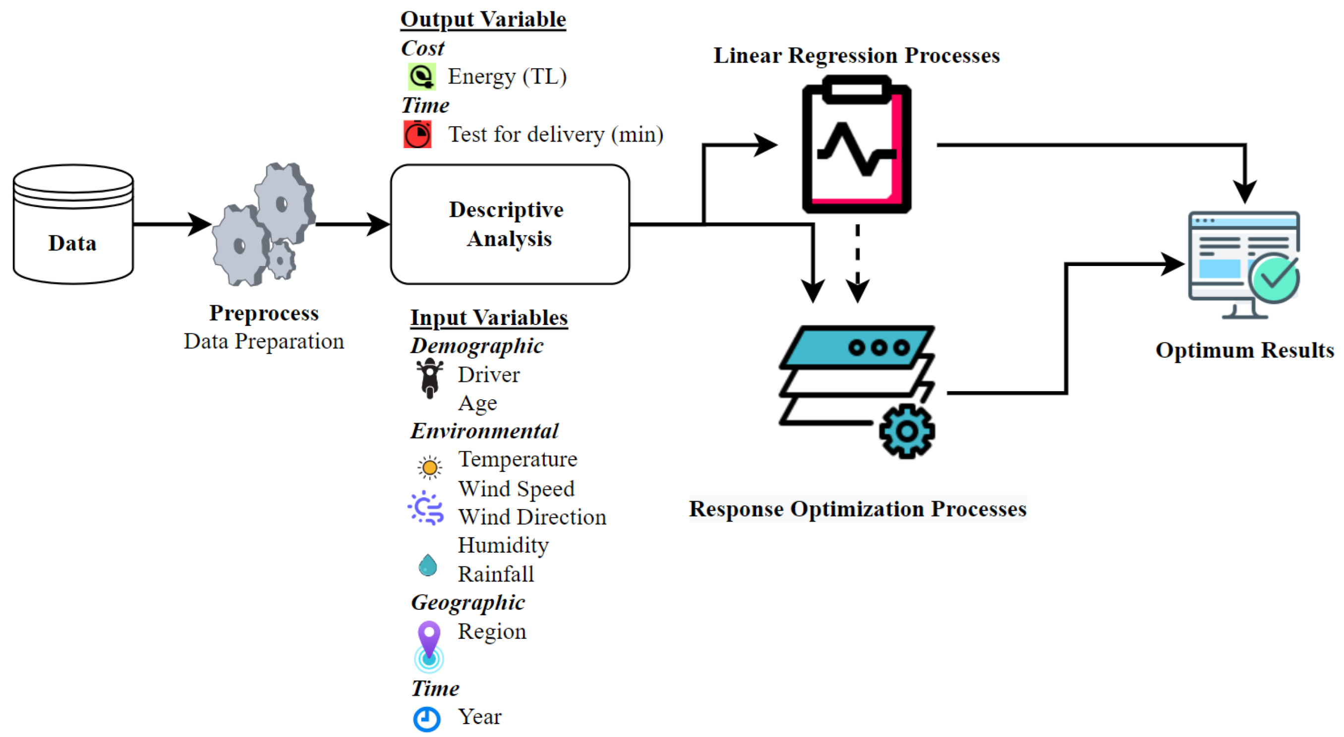
The actual data from e-scooter trial applications conducted by the Turkish Postal Service in 12 different cities of Turkey were used in this study. Among the pilot cities chosen for e-scooter vehicles for mail or package delivery, Istanbul was represented as two regions: the Anatolian and European sides. The total population of these cities is approximately 37.6 million. The people of these regions constitute 44.48% of the total population of Turkey in general. In some districts of Istanbul, mail and package delivery are carried out with e-scooter vehicles by the PTT (Turkish Post Office), the official organization of Turkey [39]. The driving tests were carried out with e-scooter vehicles for more than 20 months to spread this application to different regions in Turkey. E-scooter vehicles, when used as electrically powered delivery vehicles, were planned so that their mail or package weight could not exceed approximately 2 kg. The input and output parameters, including the driver, environment, weather, energy, and time information of 6213 e-scooter test drives, were considered. Many criteria, such as the purpose of use, user age, travel route, used region, daily usage time, travel party size, and tour mode restriction, which are important for e-scooter vehicles, have been researched subjects [21]. Before statistical analysis and optimization calculation, data processing, cleaning, and missing and outlier data were removed from the primary data set, and 1558 raw data were processed. A total of nine independent and two dependent variables were considered in this study. Detailed information, including a flowchart of the methodology and the input and output parameters, of the study is given in Figure 1.
Descriptive statistics including the sample size, mean, standard deviation, minimum value, maximum value, kurtosis, and skewness of the input and output variables are provided in Table 1. Detailed descriptive statistics based on the wind direction as a categorical variable and correlations of objective variables and input parameters are shared in Appendix A.
2.2. Linear Regression for Multiple Input and Response Variables
In simple linear regression statistical analysis, a linear equation is formed that provides an estimation of data according to the independent variable and the dependent variable by measuring the effect of the independent variable on the dependent variable. Generally, a regression equation with one dependent and independent variable is formulated as follows [40]:
where represents the dependent variable, and only one regressor variable is denoted as . The regressor variable’s coefficient and the regression equation’s constant value are symbolized as and . The error (or deviation) of the actual and predicted values of the dependent variable is represented by . However, in this study, since there was more than one regressor variable and dependent variable, the regression equation of the generalized regression model was formed as follows:
where the sum of the squares of the deviations of the observation data set from the real regression line is represented by . Minimizing the function according to the values of the constants as , , …, is necessary. In that case,
and
The normalization of the least-squares equation and the regression equation with multiple independent variables were formed as follows:
For an unknown regression coefficient, equations must be created [41]. This study discusses three different regression equations covering the number of tests, energy cost, and test time objectives required for a test with an e-scooter tool (which should be considered as the number of mail or package deliveries).
2.3. Desirability Functions
The desirability value is used to verify the validity of the optimum results of linear and nonlinear regression models. Optimum values of optimization models are obtained by obtaining individual or composite values for desirability data for a single or more than one dependent variable (objective functions). This evaluates how well the responses of the combinations of independent variables meet the defined objectives. Desirability data has a range of zero to one. It is generally accepted that optimum values are obtained when the degree of desirability approaches one, which is the ideal value. Desirability values () were computed according to the following formulation [42,43]:
If the aim is to maximize the independent variable, is constructed by the following equation:
If the aim is to minimize the independent variable, is constructed by the following equation:
If the objective function is computed for a target value, is constructed by the following equation:
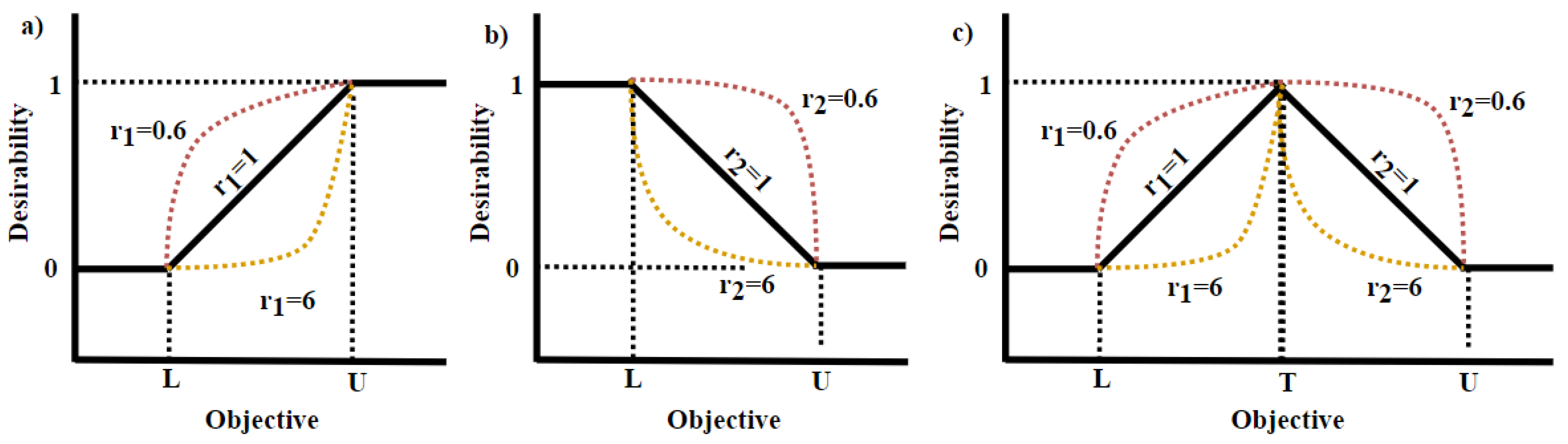
where and are the upper and lower limit values of the desired objective function equation, respectively. The parameters and express the importance of the objective function equations being close to the desired data [44]. Individual or composite desirability is calculated using a desirability function or utility transfer function to approximate the objectives of the responses. A weight value is preferred to determine how much emphasis should be placed on the dependent variable or objective function to reach its target value. The composite desirability data are calculated using the weighted geometric mean of individual desires for the dependent variables [45]. The degree of desirability of the optimization models containing different objectives of the independent variables and the variation of their and values are shown in Figure 2. An increase in and values causes the desirability degrees to be shallow unless they approach the target of the objective function [46].
Optimal settings for the independent variables were determined by maximizing the degree of compound desirability. Optimization models have been developed considering the limits of input variables for the plot regions where the e-scooter application is planned with linear response regression models. The mathematical equations of multi-objective optimization models are discussed later in this section.
2.4. Optimization Models
Generally, optimization models are defined as the expression of real-life problems in a mathematical form. There is at least one decision variable in each optimization model. These decision variables are expressed with the term . The objective function equation of a mathematical optimization model given the decision variable as is formed as follows [47]:
where denotes the coefficient of the decision variables with [48]. If the term is a cost, it tries to minimize the objective function; otherwise, if the term is a revenue, it tries to maximize the objective function. Each optimization model has a boundary of decision variables [49]. These restrictions are defined as constraints in any optimization model. In a mathematical model, constraint equations are usually created as follows [50]:
where indicates the coefficient of the input variables (or decision variables) in the constraint’s equations. The values that form the boundaries of the constraint equations are also expressed on the right-hand side. If there is no interaction between the decision variables in optimization models, and if the decision variable types (integer, rational number, binary) cannot be expressed, the equations of these models generally behave linearly. The mathematical form of the general linear optimization model is created as follows [44]:
Since some decision variables in this study were integers, the mathematical models created in this study were required to behave like mixed integer optimization models. The hybrid (mixed) integer optimization model was built as follows [51]:
The optimization models also represent an example of a TSP (traveling salesman problem) mathematical model, since the main parameter of the decision variables in the optimization models of this study was the distributors. Solving TPSs in many regions may require a lot of time to obtain the solution while using branch and bound methods so that the optimal results of the decision variables are integers. Sometimes, the optimal solution may not be obtained. For this reason, for a TSP mathematical model to quickly find a solution the answer is not optimal, or heuristics that lead to the best solution are applied. A heuristic TSP mathematical model occurs as follows [52]:
where uij is used to sort the order in which nodes appear in drivers’ travel tours [53]. The decision variable in the above mathematical model must comply with the following criteria:
The objective function of the mathematical model of the present research comprised the equation obtained from the linear response regression statistical model. Independent variables were defined as decision variables affecting the objective functions. The TSP and mixed integer optimization model were as follows [43]:
where represents the type of input variables and includes the values of the input or independent variables. These mathematical models are also referred to as multi-objective optimization models using the same independent variables of three different objective functions and the same limit values of these variables. This study’s mathematical and statistical analysis was performed with the statistical program Minitab version 19.
3. Results
In this study, the response regression optimization technique was used to obtain numerical results of the statistical and optimization models of dependent and independent variables. Numeric results of dependent variables and mathematical models are discussed in the subsections of this section.
3.1. Energy Cost
Currently, many types of vehicles are used for post or mail delivery. Authorized institutions generally assign these vehicle types’ physical and technological characteristics according to the package type distributed or city planning. However, the most significant expense of traditional delivery vehicles used in mail or package delivery is determined as energy consumption. This study considered the energy costs of e-scooter vehicles that use electrical energy, unlike traditional delivery vehicles. Postal service organizations for mail or package delivery with a particular physical feature prefer e-scooter delivery vehicles. E-scooter delivery vehicles, which carry out their operations using electrical energy, operate at three times less cost than traditional vehicles [39]. However, some factors, such as wind speed and temperature, were not considered in the energy consumption costs for other vehicles. In this study, the energy consumption costs of e-scooter vehicles were calculated by increasing the number of factors included. Table 2 shows the statistical results of the independent factors that affect the energy costs of e-scooter vehicles used for package or mail delivery.
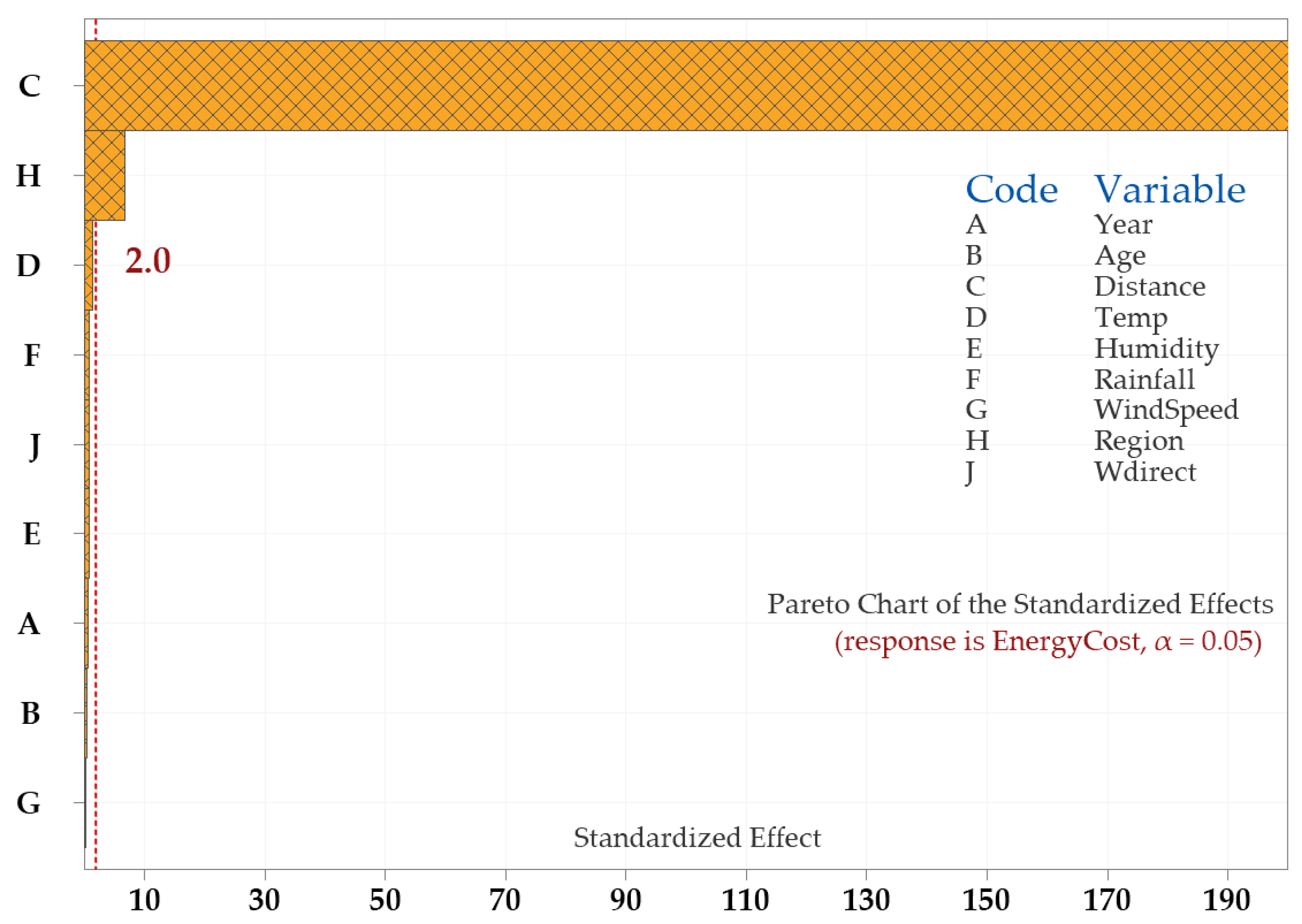
From the independent variables, the distance of the delivery address, regions where the delivery addresses were located, and wind direction were directly influential on the energy consumption of e-scooter vehicles. Statistically significant variables included degrees of time zone, distance, temperature, rainfall, and region factors were calculated with p-values of 0.053, 0.001, 0.0033, 0.044, and 0.042, respectively. Parameters such as driver age, humidity, and wind direction indirectly affected energy consumption by taking into account 10% margins of error. A standardized effect graph of the parameters that directly or indirectly affected energy consumption is shown in Figure 3.
A Pareto chart (standardized effect) was preferred to determine the magnitude and importance of the impact of independent variables. Bars crossing the baseline (baseline value calculated as 2 for this study) in this graph were considered statistically significant. Bars representing factors C (distance), H (region), and D (temperature) in this study crossed the reference line at 2.0. These factors were statistically significant at the p < 0.05 level in the current model and had an effect on the dependent variable. The effect of variable C (distance), one of the independent variables that had an indirect or direct impact on the energy cost, appeared to be very large compared to the other factors.
3.2. Test Time for Delivery of Packages or Mail
The time factor, another independent variable in the data set of this study, was taken into account and measured in minutes. The term time is expressed as the completion time of the delivery process of a package or post item made by an e-scooter under different values of different factors. In this study, the effects of eight other independent variables on the delivery time of the preferred e-scooter vehicle for mail or package delivery are explained in Table 3.
Five of the nine independent factors directly influenced the delivery time of e-scooter vehicles. Statistical impact power values of driver age, distance, time of datasets, wind speed, and test regions were calculated with p-values of 0.02, 0.001, 0.001, 0.043, and 0.001, respectively. The wind direction factor was partially but strongly influential on delivery time, while the N (p; 0.042), NE (p; 0.030), and W (p; 0.057) wind directions directly influenced the delivery time, but the other direction types indirectly affected the delivery time. The standardized effect graph on the time parameter required for deliveries with the e-scooter vehicle of the independent variables is shown in Figure 4. A standardized effect graph (Pareto graph), expressing the absolute values of the effects of the independent variables, determines which independent variables have the most significant and potent effects. However, the direction of the impact of the independent variables on the dependent variable, and whether it increases or decreases the value of the independent variable, was not determined. For this reason, coefficient data were examined to examine the magnitude and direction of the effects of independent variables.
Based on the standardized effect graph, factors A (year), B (age), C (distance), H (region), and G (wind speed) affected the delivery time. The cross-reference line was calculated as 2.0 for this dependent variable. The year (Coeff.; −0.913), age (Coeff; −0.02061), temperature (Coeff.; −0.0038), wind speed (Coeff.; −0.210), and humidity (Coeff.; −0.00884) parameters had the opposite effect on the dependent variable among these factors. Other factors had a directly proportional impact on the dependent variable. For example, it was observed that the delivery time increased as the driver’s age increased and the delivery time decreased as the wind speed increased.
3.3. Optimization Outputs Based on the Desirability Value
The objective functions of the optimization models of this study were determined as the energy cost and delivery time required for delivery with e-scooter vehicles. However, the test times that limited these two parameters were made with the e-scooter tool and are expressed as distributed packages or mail. Since the test drives did not include any packages or mail, the number of test drives was handled indirectly, not directly, as it only affected the other two parameters. For this reason, while the direction of cost and time parameters was the minimum in mathematical modeling, the number of test drives was considered the maximum. The value ranges and settings in the mathematical modeling of objective functions are shown in Table 4.
Using the same independent variables of three different objective functions and the same limit values of these variables, the optimum values of these mathematical models were measured using their degree of desirability. While the direction of two of the three objectives was the minimum, one was the maximum; it was, therefore, difficult to obtain optimum results with the same limit values of the same independent variables. This was because the linear objective function and constraint equations acted as a nonlinear optimization model for three different purposes. The single optimum values of decision variables of the optimization models (multiple response prediction) that carried out all three objectives are shared in Table 5.
The optimum values of three different objective functions that used the same independent or decision variables are given in Table 6. The optimum values in the feasible solution set were obtained as the number of tests (3.703~4), the delivery time of products was 3.747 min, and the energy cost required for a product was TRY 0.0197.
SE Fit, CI, and PI values were also calculated to verify the validity of the optimum results of the objective functions. SE Fit values for the trial ride number, time, and energy cost parameters were calculated as 0.183, 0.650, and 0.00146, respectively. The CI values of these three objectives were analyzed as 3.344–4.063, 2.473–5.021, 0.0246, and 0.0819, respectively. PI data were expressed as a feasible solution set containing the optimum values of the dependent variables. In other words, the optimum values of the independent variables could take any value in the PI set. Generally, the data range of the PI solution set was larger than the CI data range. The reason for this was that if an optimization model contains more than one objective function, it is inevitable that the data ranges of the PI solution set will expand.
The validity of the optimum results obtained using the same independent variables of all three objectives was measured using the degree of desirability and the PI and CI intervals. This performance value varied between 0 and 1, with the best results of the mathematical modeling obtained in terms of the direction of the objective functions as the degree of desirability approaches 1. The optimum values of the 50 best results according to the desirability degrees of the mathematical models developed in this study are explained in Table A3 in Appendix A.
The averages of the optimum values of the objective functions were calculated as 2.83 (rounded to 3) for the number of tests, 2.87 (number of tests must be an integer; rounded the test number to 3) for the delivery time, and 0.0208 for the energy cost required for delivery. The energy cost of a distance of approximately 100 m (or per minute) was calculated as approximately TRY 0.021. In another study, the total cost required for delivering a package or a mail was expressed as TRY 0.51 without specifying the distance rate [39]. The approximate charging fee for one trip was USD 2.5, provided an e-scooter was rented for five trips without limiting any other working distance and time in a study [54]. In another study, electric micro-mobility vehicles used only for staff travel costed approximately USD 0.39 per minute, including energy, maintenance, and operating processes [55]. The power consumed, tariff rate, and service charges were calculated by the e-scooter supplier as a total of INR 13 (approximately USD 0.16) [56]. In another study, the researchers emphasized that the energy cost per km in test drives with e-bikes varies was between 0.036 and EUR 0.194 [23]. The optimum energy cost of Turkish postal service unit e-scooter vehicles for parcel or mail delivery was approximately TRY 10.08 for a distance of 48 km with 8 h of work per day. For the first 50 feasible results, only the Konya, Kayseri, Uşak, Trabzon, and Kocaeli regions with 12 different cities were included. These regions are essential in representing other regions in the geography of Turkey, as the cities are located in five of Turkey’s seven central regions (inner Anatolia, eastern Anatolia). As a result of the optimum results of the independent variables, the city where the desirability level was maximum was Trabzon.
4. Discussion
E-scooter test drives were carried out in different regions to popularize the use of e-scooters in the post or mail delivery sector by the Turkish postal service unit. In this study, time and energy costs, two of the most important factors taken into account in the mail or package delivery sector, were calculated using data from these test drives. The data for these two factors were obtained by considering the trial driving numbers to gain statistical significance and the independent variables. The effects of both the number of trial runs and the energy and time parameters according to the desirability degrees of the optimization models of the optimum results obtained are shown in Figure 5.
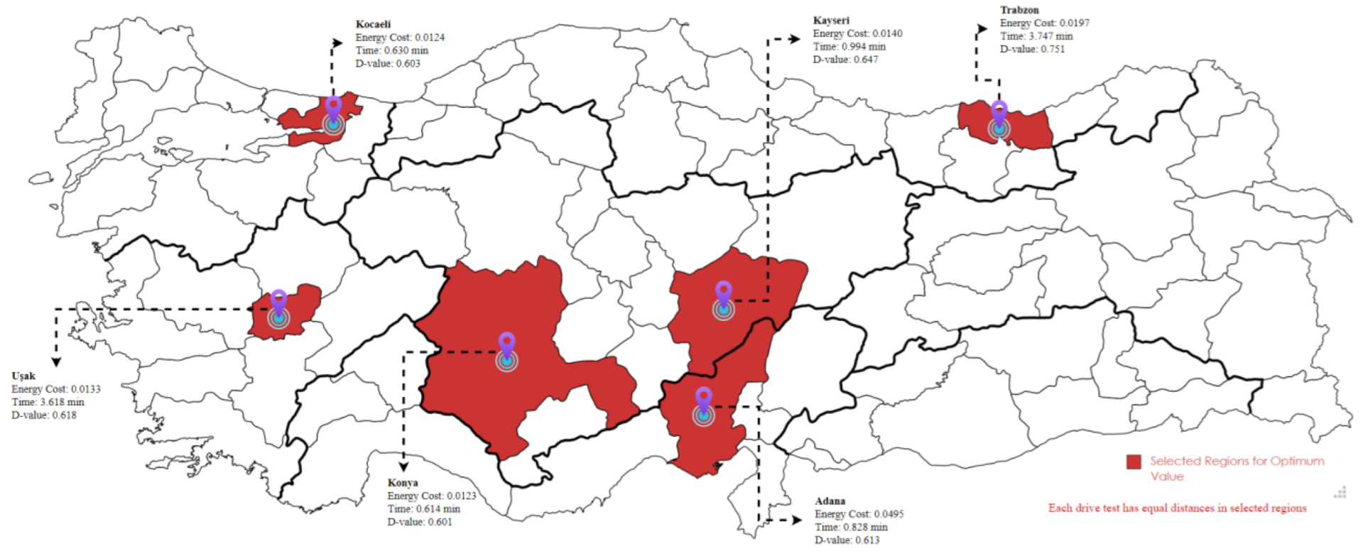
Considering the effects of independent variables, the best performance values of the optimum results obtained according to the desirability levels of the optimization models stood out in six different provinces. The data from the cities with optimum values are shown in Figure 6 (the graphic design of this map was retrieved from https://www.mapchart.net (accessed on 19 December 2022) [57]). According to the degree of desirability, the best results were obtained in the city of Trabzon, with a value of 0.71. The city of Trabzon is located in the northeast of Turkey. The most important feature of this region is that roads and settlements have more obstacles than other cities (for the areas considered in this study). Nine different drivers in this city made a total of 265 attempts. A driver made 13 trials with the e-scooter vehicle in one day at most out of 60 test runs on different days.
The desirability degrees of the Adana, Kayseri, Kocaeli, Konya, and Uşak regions, among the other provinces with high desirability degrees, were calculated as 0.613, 0.647, 0.603, 0.614, and 0.618, respectively. The minimum energy cost required for package delivery in these provinces was TRY 0.0123, which belonged to the Izmir region. Other parameters were calculated as the distance traveled by e-scooter vehicles in the areas where the optimum values were obtained. While the minimum value of the delivery time of the e-scooter vehicle used for delivering a package or mail belonged to the Kocaeli region, the delivery time taken to cover 0.098 m was calculated as 0.63 min. One study emphasized that e-scooter vehicles used for transportation can cover 0.77 miles in 7.55 min. This study revealed that it would take 5.97 min to cover 1 km with an e-scooter [58]. The city of Konya is located in the central region of Turkey. Unlike Trabzon, the layout and roads are more regular and have fewer slopes, unlike the city of Trabzon.
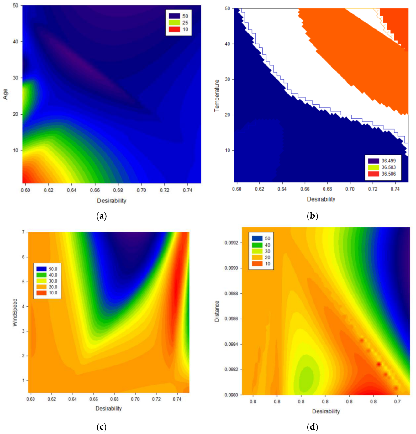
Counterplots of decision (independent) variables are shown in Figure 7, together with the statistical analyses performed to measure the effect of independent variables (without interactions of factors) on dependent variables. These plots dealt with the impact of independent variables on energy and time parameters. Counterplots showing the effects of independent factors on the degree of desirability resulting from interactions with each other are shared in Appendix A.
The age factor, expressed as the independent demographic variable of e-scooter drivers, directly affected the degree of desirability. According to the counterplot, it can be observed that there was an increase in the degree of desirability with the rise of age above a certain level. This proportionality was not observed between the temperature factor and the degree of desirability. There was a discrete distribution in the results obtained in the interaction between temperature and desirability. There was a nonlinear relationship between wind speed and desirability degrees. While the continuous increase in wind speed increased the desirability levels to a certain level, an excessive increase in wind speed caused a decrease in the desirability level. The fluctuations between such results have a significant effect on obtaining optimum results. The situation created by the impact of wind speed on the degree of desirability was also observed in the distance factor.
5. Conclusions
Many factors, such as the spread of e-commerce, formation of complex logistics networks, space of complex constructions, and changes in the physical structure of roads, directly or indirectly affect mail or package delivery services. The postal service has to implement changes in its internal dynamics to find ways to eliminate the effects of such factors. Today, in postal or package delivery services, most products are delivered to customers using traditional vehicles such as trucks, vans, pickups, motorcycles, etc. Postal delivery companies tend to reduce their vehicle sizes and turn to micro-mobility vehicles that are faster and more cost-effective to overcome the abovementioned problems, especially over short distances and in dense urban centers.
There are two crucial problems postal delivery companies face in delivering the products to the customer: the energy cost and delivery time. Delivery companies aim to shorten the delivery time and save energy costs with vehicles that require small batteries, such as e-scooters and e-bikes, which are micro-mobility vehicles. In addition, environmental sensitivity analyses of traditional vehicles used for package or mail delivery show a negative trend compared to micro-mobility delivery vehicles. In the analysis of some studies, micro-mobility vehicles, which provide many benefits in terms of the environment, economy, and energy use, also contribute to reducing traffic density. Daily traffic congestion in residential areas significantly increases the fuel consumption and carbon emissions of distribution vehicles and causes delays in the delivery of products to customers [59].
This study analyzed the cost, energy use, and environmental contributions of e-scooter vehicles for postal or package delivery by the PTT, an official institution of Turkey. In this study, nine independent factors were examined, and the effects of these factors on e-scooter vehicle use, package or mail delivery time, and energy cost were examined. To popularize the use of e-scooters, in this study, a response optimization regression method was developed using data from test drives in 12 cities. This study concluded using a statistical analysis that driver age (p; 0.002), time zone (p; 0.001), distance (p; 0.001), wind speed (p; 0.043), and delivery region (p; 0.001) had a direct effect on delivery time, while time zone (p;0.053), distance (p; 0.001), area (or region) (p; 0.001), temperature (p; 0.0033), and rainfall (p;0.044) factors had a direct effect on the energy cost.
Based on the statistical analysis results of the study, the factors of year, age, distance, region, and wind speed directly affected the delivery time. Considering the cross-reference line of 2.0 for the delivery time, which was defined as the dependent variable, year (Coeff; −0.913), age (Coeff; −0.02061), temperature (Coeff; −0.0038), wind speed (Coeff; −0.210) and humidity (Coeff; −0.00884) parameters had a negative effect on the dependent variable. It was determined that the delivery time increased as the driver’s age increased and the delivery time decreased as the wind speed increased, with a directly proportional effect of other factors on the dependent variable. The other dependent variable, the energy cost, was positively affected by the year, distance, temperature, humidity, precipitation, and wind speed. The cross-reference line for this dependent variable was considered as 2.0. The parameters of year (Coeff; 0.000385), distance (Kats; 0.054207), temperature (Coeff; 0.000068), humidity (Coeff; 0.000022), precipitation (Coeff; 0.000038), and wind speed (Coeff; 0.000121) positively affected the dependent variable. Only the age (Coeff; −0.000015) and region (Coeff; −0.013091) parameters had a negative impact on the energy cost required for delivery.
By calculating the optimum data for the dependent and independent variables, the effects of the interactions of the variables on the energy cost and delivery time could be discussed. The optimal results were tested using desirability degrees to verify the validity of the optimum results of the mathematical models. The data concerning the optimum values of the objective functions in the mathematical models were calculated as 2.83 (rounded up to 3) for the number of tests, 2.87 for the delivery time, and 0.0208 for the energy cost required. The optimum energy cost for a distance of approximately 100 m (or per minute) was calculated as approximately TRY 0.021.
This study had some limitations and prerequisites. Although the data on the batteries of the e-scooter vehicles were not taken into account, batteries were full during the test drives. The charging time of the batteries was not taken into account in the trial runs. Another limit was the slope information of the roads used by e-scooter vehicles for testing in the regions considered in the study. The effects of these data on driving times and energy consumption could not be measured. The third limitation was that data on physical structures, such as the weight and height of e-scooter drivers, were not used in this research. A final limitation of this study was the absence of legal regulations regarding e-scooter transportation. For this reason, the safety of e-scooter drivers was not discussed in this study. There is a need for studies that argue that this problem is essential for drivers using electric vehicles, such as e-scooters, for negative situations that they may encounter during travel [60].
As a result, in terms of the environment, economy, and energy consumption, using micro-mobility vehicles, such as e-scooters, provides significant advantages in the package and postal transportation sector in densely populated areas. This study concluded that micro-mobility vehicles would contribute in many areas due to test applications in 12 cities in terms of both delivery time and energy cost of the e-scooter vehicle in mail or package transportation.
Funding
This research received no external funding.
Institutional Review Board Statement
Not applicable.
Informed Consent Statement
Not applicable.
Data Availability Statement
Not applicable.
Conflicts of Interest
The author declares no conflict of interest.
Appendix A
The correlation values of the dependent and independent variables in the preference of using e-scooter vehicles in the mail or package delivery are given in Table A1. The correlation values between the variables were analyzed by evaluating the correlation values in three different categories. If the correlation value between variables was between 0.1 and 0.3 it was considered a weak correlation; between 0.3 and 0.5 was a moderate correlation, and between 0.5–0.9 was a strong correlation [61].

Table A1.
The values of correlations based on the pairwise Pearson correlation test.
| Sample 1 | Sample 2 | Sample Size | Correlation | 95% CI for ρ | p-Value | Status |
|---|---|---|---|---|---|---|
| Age | Year | 1578 | 0.70 | (0.021, 0.119) | 0.005 | Strong |
| Distance | Year | 1578 | 0.38 | (−0.012, 0.087) | 0.136 | Moderate |
| Temperature | Year | 1578 | 0.27 | (0.229, 0.321) | 0.000 | Weak |
| Humidity | Year | 1578 | −0.17 | (−0.225, −0.129) | 0.000 | Weak |
| Rainfall | Year | 1578 | −0.27 | (−0.077, 0.022) | 0.276 | Weak |
| WindSpeed | Year | 1578 | −0.14 | (−0.153, −0.055) | 0.000 | Weak |
| Test | Year | 1578 | 0.19 | (−0.030, 0.068) | 0.449 | Weak |
| EnergyCost | Year | 1578 | 0.42 | (−0.007, 0.091) | 0.095 | Moderate |
| DeliveryTime | Year | 1578 | −0.20 | (−0.052, 0.047) | 0.925 | Weak |
| Distance | Age | 1578 | 0.11 | (0.061, 0.158) | 0.000 | Weak |
| Temperature | Age | 1578 | 0.15 | (0.106, 0.202) | 0.000 | Weak |
| Humidity | Age | 1578 | 0.30 | (−0.019, 0.080) | 0.228 | Moderate |
| Rainfall | Age | 1578 | 0.23 | (−0.027, 0.072) | 0.369 | Weak |
| WindSpeed | Age | 1578 | 0.32 | (−0.017, 0.082) | 0.198 | Moderate |
| Test | Age | 1578 | 0.16 | (−0.033, 0.066) | 0.520 | Weak |
| EnergyCost | Age | 1578 | 0.11 | (0.061, 0.159) | 0.000 | Weak |
| DeliveryTime | Age | 1578 | 0.55 | (0.006, 0.104) | 0.028 | Moderate |
| Temperature | Distance | 1578 | 0.16 | (0.120, 0.216) | 0.000 | Weak |
| Humidity | Distance | 1578 | −0.64 | (−0.113, −0.014) | 0.012 | Strong |
| Rainfall | Distance | 1578 | −0.22 | (−0.072, 0.027) | 0.376 | Weak |
| WindSpeed | Distance | 1578 | −0.49 | (−0.098, 0.000) | 0.052 | Moderate |
| Test | Distance | 1578 | 0.22 | (−0.027, 0.071) | 0.378 | Weak |
| EnergyCost | Distance | 1578 | 0.99 | (0.991, 0.993) | 0.000 | Strong |
| DeliveryTime | Distance | 1578 | 0.92 | (0.912, 0.928) | 0.000 | Strong |
| Humidity | Temperature | 1578 | −0.27 | (−0.264, −0.170) | 0.000 | Weak |
| Rainfall | Temperature | 1578 | 0.27 | (−0.022, 0.076) | 0.280 | Weak |
| WindSpeed | Temperature | 1578 | 0.19 | (−0.030, 0.069) | 0.441 | Weak |
| Test | Temperature | 1578 | 0.59 | (0.110, 0.207) | 0.000 | Moderate |
| EnergyCost | Temperature | 1578 | 0.77 | (0.129, 0.225) | 0.000 | Strong |
| DeliveryTime | Temperature | 1578 | 0.57 | (0.109, 0.205) | 0.000 | Moderate |
| Rainfall | Humidity | 1578 | 0.81 | (0.031, 0.129) | 0.001 | Strong |
| WindSpeed | Humidity | 1578 | 0.52 | (0.002, 0.101) | 0.040 | Moderate |
| Test | Humidity | 1578 | 0.07 | (−0.042, 0.056) | 0.783 | Weak |
| EnergyCost | Humidity | 1578 | −0.61 | (−0.110, −0.012) | 0.015 | Strong |
| DeliveryTime | Humidity | 1578 | −0.98 | (−0.146, −0.049) | 0.000 | Strong |
| WindSpeed | Rainfall | 1578 | −0.51 | (−0.100, −0.001) | 0.044 | Moderate |
| Test | Rainfall | 1578 | −0.20 | (−0.069, 0.029) | 0.425 | Weak |
| EnergyCost | Rainfall | 1578 | −0.13 | (−0.063, 0.036) | 0.593 | Weak |
| DeliveryTime | Rainfall | 1578 | −0.19 | (−0.068, 0.030) | 0.451 | Weak |
| Test | Wind Speed | 1578 | 0.76 | (0.027, 0.125) | 0.002 | Strong |
| EnergyCost | Wind Speed | 1578 | −0.49 | (−0.098, 0.000) | 0.052 | Moderate |
| DeliveryTime | Wind Speed | 1578 | −0.25 | (−0.075, 0.024) | 0.314 | Weak |
| EnergyCost | Test | 1578 | 0.28 | (−0.021, 0.077) | 0.262 | Weak |
| DeliveryTime | Test | 1578 | 0.66 | (0.017, 0.115) | 0.008 | Strong |
| DeliveryTime | EnergyCost | 1578 | 0.91 | (0.909, 0.925) | 0.000 | Strong |
Abbreviation: CI, confidence interval; ρ, correlation coefficient.
Descriptive statistical data of the influential factors in terms of time and energy costs of e-scooter vehicles in the mail or package delivery were analyzed. The sample size, mean, standard error, standard deviation, minimum value, maximum value, kurtosis, and skewness of other variables were calculated according to the wind direction parameters, which were categorical variables from the independent factors. The region factor was not included in the descriptive statistical analysis among the independent variables. The independent variable data according to the wind direction are shared in Table A2.
Table A2.
The descriptive statistics based on the wind direction variable as a categorical input factor.
Table A2.
The descriptive statistics based on the wind direction variable as a categorical input factor.
| Variable | Wdirect | TCS | Mean | SE Mean | StDev | Min | Max | Skewness | Kurtosis |
|---|---|---|---|---|---|---|---|---|---|
| Year | E | 144 | 2021 | 0.044 | 0.522 | 2020 | 2022 | −1.060 | 0.020 |
| (Test time) | N | 88 | 2021 | 0.056 | 0.529 | 2020 | 2022 | −1.610 | 1.740 |
| NE | 422 | 2021 | 0.026 | 0.535 | 2020 | 2022 | −1.610 | 1.670 | |
| NW | 430 | 2021 | 0.024 | 0.488 | 2020 | 2022 | −1.000 | −0.420 | |
| S | 139 | 2021 | 0.044 | 0.519 | 2020 | 2022 | −1.160 | 0.280 | |
| SE | 99 | 2021 | 0.063 | 0.623 | 2020 | 2022 | −1.240 | 0.460 | |
| SW | 101 | 2021 | 0.046 | 0.467 | 2020 | 2022 | −1.360 | 0.620 | |
| W | 155 | 2021 | 0.044 | 0.543 | 2020 | 2022 | −1.220 | 0.510 | |
| Age of | E | 144 | 29.583 | 0.962 | 11.548 | 18.000 | 56.000 | 1.150 | −0.080 |
| Drivers | N | 88 | 30.580 | 1.460 | 13.710 | 19.000 | 56.000 | 1.060 | −0.600 |
| NE | 422 | 30.611 | 0.612 | 12.580 | 18.000 | 56.000 | 0.880 | −0.740 | |
| NW | 430 | 28.160 | 0.510 | 10.582 | 18.000 | 56.000 | 1.490 | 1.020 | |
| S | 139 | 27.281 | 0.889 | 10.481 | 18.000 | 56.000 | 1.250 | 0.030 | |
| SE | 99 | 28.040 | 1.080 | 10.790 | 18.000 | 56.000 | 1.300 | 0.480 | |
| SW | 101 | 28.450 | 1.150 | 11.560 | 18.000 | 56.000 | 1.440 | 0.660 | |
| W | 155 | 26.981 | 0.775 | 9.644 | 18.000 | 56.000 | 1.810 | 2.340 | |
| Distance | E | 144 | 2.321 | 0.150 | 1.797 | 0.181 | 9.682 | 1.490 | 2.460 |
| (km) | N | 88 | 1.866 | 0.173 | 1.618 | 0.182 | 9.492 | 1.910 | 5.230 |
| NE | 422 | 1.979 | 0.080 | 1.648 | 0.098 | 9.392 | 1.630 | 3.140 | |
| NW | 430 | 1.873 | 0.067 | 1.384 | 0.136 | 8.827 | 1.530 | 3.290 | |
| S | 139 | 1.836 | 0.129 | 1.526 | 0.181 | 7.960 | 1.830 | 3.730 | |
| SE | 99 | 1.688 | 0.136 | 1.358 | 0.190 | 8.171 | 2.450 | 7.840 | |
| SW | 101 | 2.234 | 0.190 | 1.905 | 0.208 | 8.703 | 1.610 | 2.280 | |
| W | 155 | 2.079 | 0.130 | 1.613 | 0.130 | 9.883 | 1.490 | 3.280 | |
| Temperature | E | 144 | 18.623 | 0.494 | 5.931 | 5.500 | 30.100 | −0.430 | −0.330 |
| (Average) | N | 88 | 18.261 | 0.774 | 7.263 | −0.750 | 28.750 | −0.610 | −0.420 |
| NE | 422 | 20.203 | 0.305 | 6.270 | 1.600 | 36.500 | −0.670 | −0.270 | |
| NW | 430 | 17.642 | 0.361 | 7.490 | 1.500 | 34.000 | −0.410 | −0.960 | |
| S | 139 | 20.434 | 0.743 | 8.763 | 2.100 | 32.000 | −0.540 | −1.200 | |
| SE | 99 | 18.236 | 0.695 | 6.916 | 0.300 | 29.950 | −0.190 | −0.840 | |
| SW | 101 | 17.502 | 0.771 | 7.744 | 5.200 | 30.100 | −0.330 | −1.190 | |
| W | 155 | 17.917 | 0.604 | 7.519 | 3.700 | 27.600 | −0.270 | −1.370 | |
| Humidity | E | 144 | 66.890 | 1.060 | 12.710 | 23.500 | 90.700 | −0.990 | 1.730 |
| N | 88 | 70.390 | 1.200 | 11.280 | 45.300 | 94.200 | −0.130 | −0.250 | |
| NE | 422 | 68.267 | 0.599 | 12.299 | 28.600 | 99.000 | −0.470 | 0.480 | |
| NW | 430 | 64.568 | 0.628 | 13.023 | 27.800 | 96.700 | −0.190 | 0.120 | |
| S | 139 | 69.281 | 0.951 | 11.214 | 32.400 | 92.500 | −0.670 | 0.350 | |
| SE | 99 | 68.400 | 1.080 | 10.760 | 35.200 | 92.200 | −0.410 | 0.400 | |
| SW | 101 | 67.050 | 1.150 | 11.600 | 31.900 | 88.800 | −0.730 | 0.770 | |
| W | 155 | 62.630 | 1.010 | 12.590 | 31.300 | 87.300 | 0.020 | −0.620 | |
| Rainfall | E | 144 | 4.374 | 0.617 | 7.399 | 0.100 | 33.800 | 2.670 | 6.980 |
| N | 88 | 4.897 | 0.807 | 7.571 | 0.100 | 30.300 | 2.390 | 5.200 | |
| NE | 422 | 3.391 | 0.282 | 5.801 | 0.100 | 40.200 | 3.200 | 11.620 | |
| NW | 430 | 3.003 | 0.203 | 4.214 | 0.100 | 42.800 | 3.630 | 22.810 | |
| S | 139 | 6.405 | 0.860 | 10.143 | 0.100 | 56.800 | 3.240 | 12.440 | |
| SE | 99 | 5.565 | 0.855 | 8.506 | 0.100 | 53.900 | 2.730 | 10.430 | |
| SW | 101 | 6.121 | 0.896 | 9.003 | 0.100 | 34.200 | 1.970 | 3.270 | |
| W | 155 | 6.395 | 0.589 | 7.336 | 0.100 | 33.200 | 2.280 | 5.780 | |
| Wind Speed | E | 144 | 1.523 | 0.044 | 0.523 | 0.700 | 3.300 | 0.650 | 0.660 |
| (Average) | N | 88 | 1.498 | 0.065 | 0.609 | 0.800 | 4.300 | 2.250 | 7.540 |
| NE | 422 | 1.666 | 0.037 | 0.758 | 0.500 | 6.100 | 2.310 | 8.860 | |
| NW | 430 | 1.571 | 0.044 | 0.908 | 0.600 | 7.000 | 2.150 | 6.410 | |
| S | 139 | 1.780 | 0.072 | 0.843 | 0.600 | 6.200 | 1.490 | 4.580 | |
| SE | 99 | 1.528 | 0.081 | 0.806 | 0.800 | 6.500 | 3.530 | 17.210 | |
| SW | 101 | 1.415 | 0.047 | 0.471 | 0.700 | 3.300 | 0.870 | 1.590 | |
| W | 155 | 1.444 | 0.059 | 0.729 | 0.700 | 5.700 | 3.010 | 14.020 | |
| Test | E | 144 | 1.875 | 0.085 | 1.023 | 1.000 | 5.000 | 1.010 | 0.200 |
| Drive | N | 88 | 1.841 | 0.111 | 1.038 | 1.000 | 5.000 | 1.080 | 0.240 |
| NE | 422 | 1.912 | 0.054 | 1.100 | 1.000 | 5.000 | 1.140 | 0.560 | |
| NW | 430 | 1.830 | 0.052 | 1.078 | 1.000 | 5.000 | 1.230 | 0.710 | |
| S | 139 | 2.281 | 0.131 | 1.547 | 1.000 | 7.000 | 1.280 | 1.140 | |
| SE | 99 | 1.909 | 0.113 | 1.126 | 1.000 | 5.000 | 1.010 | −0.090 | |
| SW | 101 | 1.634 | 0.094 | 0.946 | 1.000 | 5.000 | 1.520 | 1.660 | |
| W | 155 | 1.819 | 0.079 | 0.977 | 1.000 | 5.000 | 1.130 | 0.850 | |
| Energy | E | 144 | 0.127 | 0.008 | 0.098 | 0.010 | 0.525 | 1.450 | 2.290 |
| Cost | N | 88 | 0.102 | 0.009 | 0.088 | 0.010 | 0.515 | 1.920 | 5.290 |
| NE | 422 | 0.108 | 0.004 | 0.089 | 0.005 | 0.510 | 1.610 | 3.100 | |
| NW | 430 | 0.103 | 0.004 | 0.075 | 0.007 | 0.479 | 1.500 | 3.150 | |
| S | 139 | 0.105 | 0.008 | 0.089 | 0.004 | 0.432 | 1.620 | 2.490 | |
| SE | 99 | 0.091 | 0.007 | 0.073 | 0.010 | 0.430 | 2.400 | 7.410 | |
| SW | 101 | 0.122 | 0.010 | 0.105 | 0.011 | 0.472 | 1.620 | 2.280 | |
| W | 155 | 0.113 | 0.007 | 0.087 | 0.007 | 0.536 | 1.480 | 3.260 | |
| Time | E | 144 | 11.281 | 0.674 | 8.085 | 1.000 | 47.000 | 1.630 | 3.190 |
| (min) | N | 88 | 9.622 | 0.754 | 7.073 | 2.000 | 46.270 | 2.300 | 8.030 |
| NE | 422 | 10.021 | 0.356 | 7.317 | 1.000 | 43.000 | 1.500 | 2.550 | |
| NW | 430 | 9.853 | 0.312 | 6.461 | 1.000 | 41.200 | 1.460 | 2.920 | |
| S | 139 | 10.098 | 0.539 | 6.358 | 2.000 | 36.610 | 1.660 | 3.580 | |
| SE | 99 | 8.406 | 0.628 | 6.253 | 1.000 | 38.810 | 2.540 | 8.910 | |
| SW | 101 | 11.040 | 0.851 | 8.554 | 1.000 | 37.000 | 1.360 | 1.210 | |
| W | 155 | 10.990 | 0.631 | 7.853 | 1.000 | 49.760 | 1.630 | 3.700 |
Abbreviations: TCS, total count of the sample set; SE, standard error; Std, standard deviation; Min, minimum value; Max, maximum value; Wdirect, wind direction; N, north; NE, northeast; NW, northwest; S, south; SE, southeast; SW, southwest; W, west; min, minute.
The optimum values of the objective function and decision variables in the mathematical models developed in this study are explained in Table A3 and were calculated using the best 50 results according to the desirability levels of the optimization model.
Table A3.
The optimum values of objective functions and decision variables based on the desirability values.
Table A3.
The optimum values of objective functions and decision variables based on the desirability values.
| Fit | Temp | Age | Region | Year | Distance | Wind Speed | Test | Time | Energy Cost | Desirability |
|---|---|---|---|---|---|---|---|---|---|---|
| 1 | 36.50 | 56.00 | Trabzon | 2022 | 0.098 | 7.000 | 3.703 | 3.747 | 0.0197 | 0.751 |
| 2 | 36.50 | 56.00 | Trabzon | 2022 | 0.098 | 7.000 | 3.703 | 3.747 | 0.0197 | 0.751 |
| 3 | 36.50 | 56.00 | Trabzon | 2022 | 0.098 | 7.000 | 3.703 | 3.747 | 0.0197 | 0.751 |
| 4 | 36.50 | 56.00 | Trabzon | 2022 | 0.098 | 7.000 | 3.703 | 3.748 | 0.0197 | 0.751 |
| 5 | 36.50 | 56.00 | Trabzon | 2022 | 0.098 | 7.000 | 3.703 | 3.749 | 0.0197 | 0.751 |
| 6 | 36.50 | 56.00 | Trabzon | 2022 | 0.098 | 7.000 | 3.703 | 3.749 | 0.0197 | 0.751 |
| 7 | 36.50 | 56.00 | Trabzon | 2022 | 0.098 | 1.013 | 3.703 | 5.027 | 0.0197 | 0.744 |
| 8 | 36.50 | 56.00 | Trabzon | 2022 | 0.098 | 0.507 | 3.703 | 5.135 | 0.0197 | 0.744 |
| 9 | 36.50 | 24.69 | Trabzon | 2022 | 0.098 | 7.000 | 3.637 | 4.364 | 0.0194 | 0.742 |
| 10 | 36.50 | 24.69 | Trabzon | 2022 | 0.098 | 7.000 | 3.637 | 4.364 | 0.0194 | 0.742 |
| 11 | 36.50 | 24.69 | Trabzon | 2022 | 0.098 | 7.000 | 3.637 | 4.365 | 0.0194 | 0.742 |
| 12 | 36.50 | 24.70 | Trabzon | 2022 | 0.098 | 7.000 | 3.637 | 4.366 | 0.0194 | 0.742 |
| 13 | 36.50 | 18.13 | Trabzon | 2022 | 0.098 | 7.000 | 3.623 | 4.494 | 0.0193 | 0.740 |
| 14 | 36.50 | 18.00 | Trabzon | 2022 | 0.098 | 7.000 | 3.622 | 4.496 | 0.0193 | 0.740 |
| 15 | 36.50 | 18.13 | Trabzon | 2022 | 0.098 | 1.012 | 3.623 | 5.775 | 0.0193 | 0.733 |
| 16 | 36.50 | 18.00 | Trabzon | 2022 | 0.098 | 0.507 | 3.622 | 5.883 | 0.0193 | 0.732 |
| 17 | 36.50 | 56.00 | Kayseri | 2022 | 0.098 | 7.000 | 2.631 | 0.994 | 0.0140 | 0.647 |
| 18 | 36.50 | 56.00 | Kayseri | 2022 | 0.099 | 7.000 | 2.631 | 1.000 | 0.0142 | 0.647 |
| 19 | 36.50 | 56.00 | Kayseri | 2022 | 0.098 | 7.000 | 2.631 | 1.011 | 0.0140 | 0.647 |
| 20 | 36.50 | 56.00 | Kayseri | 2022 | 0.098 | 1.012 | 2.631 | 2.275 | 0.0140 | 0.641 |
| 21 | 36.50 | 56.00 | Kayseri | 2022 | 0.098 | 0.507 | 2.631 | 2.382 | 0.0140 | 0.641 |
| 22 | 36.50 | 18.20 | Kayseri | 2022 | 0.098 | 7.000 | 2.551 | 1.741 | 0.0136 | 0.633 |
| 23 | 36.50 | 18.00 | Kayseri | 2022 | 0.098 | 7.000 | 2.550 | 1.743 | 0.0136 | 0.633 |
| 24 | 36.50 | 18.20 | Kayseri | 2022 | 0.098 | 1.013 | 2.551 | 3.019 | 0.0136 | 0.627 |
| 25 | 36.50 | 18.00 | Kayseri | 2022 | 0.098 | 0.507 | 2.550 | 3.131 | 0.0136 | 0.627 |
| 26 | 36.50 | 56.00 | Uşak | 2022 | 0.098 | 7.000 | 2.504 | 3.618 | 0.0133 | 0.618 |
| 27 | 36.50 | 56.00 | Uşak | 2022 | 0.098 | 7.000 | 2.504 | 3.620 | 0.0133 | 0.618 |
| 28 | 36.50 | 56.00 | Adana | 2022 | 0.098 | 7.000 | 2.424 | 0.828 | 0.0495 | 0.613 |
| 29 | 36.50 | 56.00 | Uşak | 2022 | 0.098 | 1.013 | 2.504 | 4.898 | 0.0133 | 0.613 |
| 30 | 36.50 | 56.00 | Adana | 2021 | 0.098 | 7.000 | 2.424 | 1.011 | 0.0495 | 0.613 |
| 31 | 36.50 | 56.00 | Uşak | 2022 | 0.098 | 0.507 | 2.504 | 5.006 | 0.0133 | 0.612 |
| 32 | 36.50 | 56.00 | Adana | 2022 | 0.098 | 3.382 | 2.424 | 1.205 | 0.0495 | 0.612 |
| 33 | 36.50 | 56.00 | Adana | 2022 | 0.098 | 3.366 | 2.424 | 1.205 | 0.0495 | 0.612 |
| 34 | 20.66 | 56.00 | Kayseri | 2022 | 0.098 | 6.875 | 2.355 | 1.021 | 0.0125 | 0.608 |
| 35 | 36.50 | 18.21 | Uşak | 2022 | 0.098 | 7.000 | 2.423 | 4.364 | 0.0129 | 0.604 |
| 36 | 36.50 | 18.00 | Uşak | 2022 | 0.098 | 7.000 | 2.423 | 4.367 | 0.0129 | 0.604 |
| 37 | 36.50 | 56.00 | Kocaeli | 2022 | 0.098 | 7.000 | 2.323 | 0.630 | 0.0124 | 0.603 |
| 38 | 36.50 | 56.00 | Kocaeli | 2021 | 0.098 | 7.000 | 2.323 | 1.011 | 0.0124 | 0.603 |
| 39 | 36.50 | 56.00 | Kocaeli | 2022 | 0.098 | 1.012 | 2.323 | 1.344 | 0.0124 | 0.602 |
| 40 | 36.50 | 56.00 | Kocaeli | 2022 | 0.098 | 0.506 | 2.323 | 1.450 | 0.0124 | 0.602 |
| 41 | 36.50 | 56.00 | Konya | 2022 | 0.098 | 7.000 | 2.309 | 0.614 | 0.0123 | 0.601 |
| 42 | 36.50 | 56.00 | Konya | 2021 | 0.098 | 7.000 | 2.309 | 1.011 | 0.0123 | 0.601 |
| 43 | 36.50 | 20.79 | Adana | 2022 | 0.098 | 6.759 | 2.349 | 1.174 | 0.0479 | 0.601 |
| 44 | 36.50 | 20.79 | Adana | 2022 | 0.098 | 6.760 | 2.349 | 1.174 | 0.0479 | 0.601 |
| 45 | 36.50 | 18.23 | Adana | 2022 | 0.098 | 7.000 | 2.344 | 1.173 | 0.0478 | 0.600 |
| 46 | 36.50 | 18.00 | Adana | 2022 | 0.098 | 7.000 | 2.343 | 1.177 | 0.0478 | 0.600 |
| 47 | 36.50 | 56.00 | Konya | 2022 | 0.098 | 1.012 | 2.309 | 1.694 | 0.0123 | 0.599 |
| 48 | 36.50 | 18.20 | Uşak | 2022 | 0.098 | 1.012 | 2.423 | 5.644 | 0.0129 | 0.598 |
| 49 | 36.50 | 56.00 | Konya | 2022 | 0.098 | 0.507 | 2.309 | 1.801 | 0.0123 | 0.598 |
| 50 | 36.50 | 18.00 | Uşak | 2022 | 0.098 | 0.507 | 2.423 | 5.755 | 0.0129 | 0.598 |
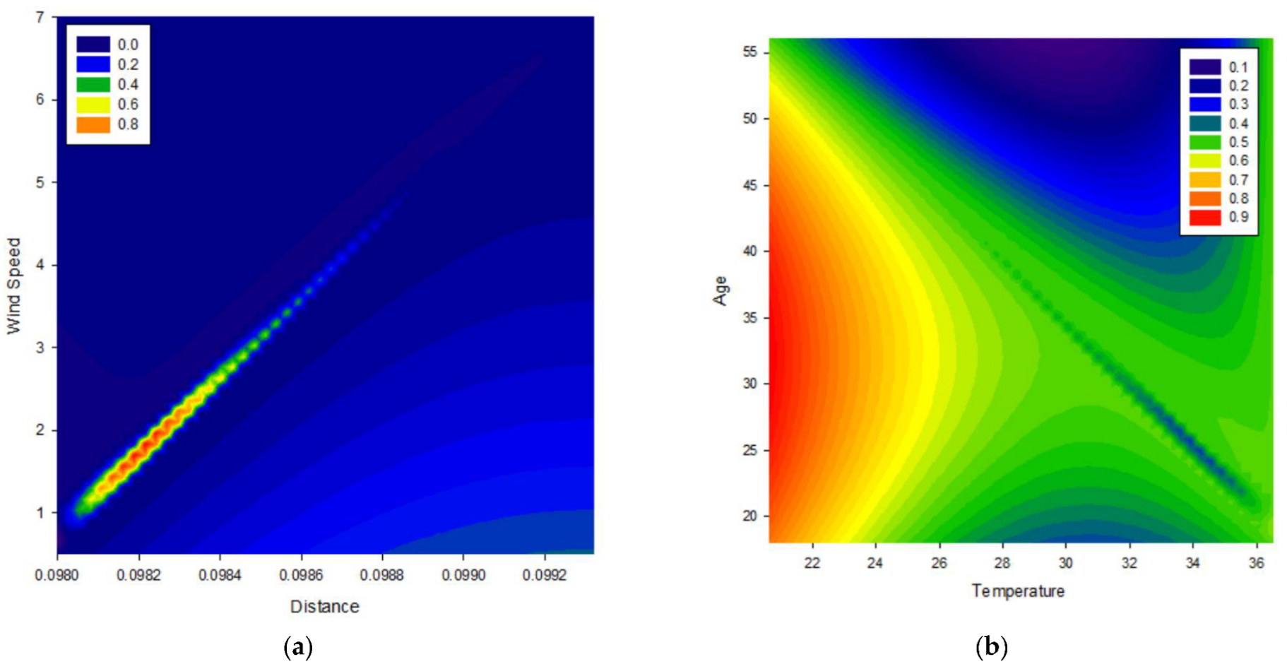
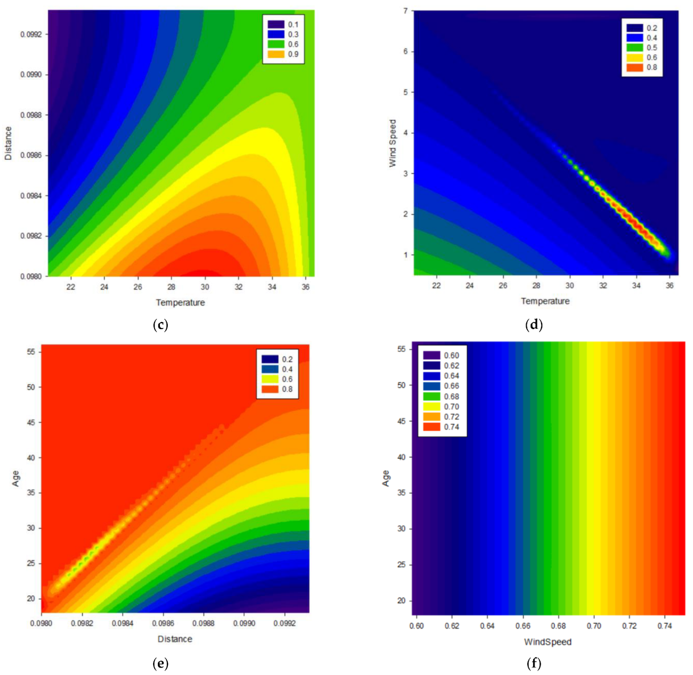
The interactions of the distance, age, temperature, and wind speed factors that do not have categorical data from the independent variables according to the desirability degree of mathematical modeling are discussed in the counterplot images in Figure A1. It was concluded that as the colors became darker in counterplot shapes, the degree of desirability increased, and the independent variables reached optimum values.
Figure A1.
The effects of independent factors (interactions of factors) on the degree of desirability: (a) windspeed–distance, (b) age–temperature (c), distance–temperature, (d) windspeed–temperature, (e) age–distance, (f) age–windspeed.
Figure A1.
The effects of independent factors (interactions of factors) on the degree of desirability: (a) windspeed–distance, (b) age–temperature (c), distance–temperature, (d) windspeed–temperature, (e) age–distance, (f) age–windspeed.


References
- de Mello Bandeira, R.A.; Goes, G.V.; Schmitz Gonçalves, D.N.; de Almeida D’Agosto, M.; de Oliveira, C.M. Electric vehicles in the last mile of urban freight transportation: A sustainability assessment of postal deliveries in Rio de Janeiro-Brazil. Transp. Res. Part D Transp. Environ. 2019, 67, 491–502. [Google Scholar] [CrossRef]
- Inac, H.; Oztemel, E. An Assessment Framework for the Transformation of Mobility 4.0 in Smart Cities. Systems 2021, 10, 1. [Google Scholar] [CrossRef]
- Hesse, M. Shipping news: The implications of electronic commerce for logistics and freight transport. Resour. Conserv. Recycl. 2002, 36, 211–240. [Google Scholar] [CrossRef]
- Tanyaş, M.; Sıcakyüz, A. İstanbul lojistik sektör analizi raporu. Müstakil Sanayici ve İşadamları Derneği Loder Derg. 2014. Available online: https://musiad.org.tr/uploads/yayinlar/arastirma-raporlari/pdf/lojistik_sektor_analizi_1_1.pdf (accessed on 19 December 2022).
- Colmenar-Santos, A.; Reino-Rio, C.; Borge-Diez, D.; Collado-Fernández, E. Distributed generation: A review of factors that can contribute most to achieve a scenario of DG units embedded in the new distribution networks. Renew. Sustain. Energy Rev. 2016, 59, 1130–1148. [Google Scholar] [CrossRef]
- Song, M.; Wu, N.; Wu, K. Energy consumption and energy efficiency of the transportation sector in Shanghai. Sustainability 2014, 6, 702–717. [Google Scholar] [CrossRef] [Green Version]
- Madlenak, R.; Madlenakova, L.; Stefunko, J. The variant approach to the optimization of the postal transportation network in the conditions of the Slovak Republic. Transp. Telecommun. J. 2015, 16, 237–245. [Google Scholar]
- Moreno, M.A.; Ortega, J.F.; Córcoles, J.I.; Martínez, A.; Tarjuelo, J.M. Energy analysis of irrigation delivery systems: Monitoring and evaluation of proposed measures for improving energy efficiency. Irrig. Sci. 2010, 28, 445–460. [Google Scholar] [CrossRef]
- Dong, H.; Fu, J.; Zhao, Z.; Liu, Q.; Li, Y.; Liu, J. A comparative study on the energy flow of a conventional gasoline-powered vehicle and a new dual clutch parallel-series plug-in hybrid electric vehicle under NEDC. Energy Convers. Manag. 2020, 218, 113019. [Google Scholar] [CrossRef]
- İnaç, H. İstanbulun kentsel lojistik analizi ve çözüm önerilerinin analitik hiyerarşi prosesi (AHP) ile değerlendirilmesi. Master’s thesis, Fen Bilimleri Enstitüsü, Ankara, Türkiye, 2012. [Google Scholar]
- Lee, M.; Chow, J.Y.J.; Yoon, G.; He, B.Y. Forecasting e-scooter substitution of direct and access trips by mode and distance. Transp. Res. Part D Transp. Environ. 2021, 96, 102892. [Google Scholar] [CrossRef]
- Liu, M.; Seeder, S.; Li, H. Analysis of e-scooter trips and their temporal usage patterns. Inst. Transp. Eng. ITE J. 2019, 89, 44–49. [Google Scholar]
- Dias, G.; Arsenio, E.; Ribeiro, P. The Role of Shared E-Scooter Systems in Urban Sustainability and Resilience during the Covid-19 Mobility Restrictions. Sustainability 2021, 13, 7084. [Google Scholar] [CrossRef]
- Javadinasr, M.; Asgharpour, S.; Rahimi, E.; Mohammadian, A.; Auld, J. Understanding Long-Term Intention for Micromobility: Insight from Shared E-Scooters in Chicago. In Proceedings of the International Conference on Transportation and Development 2022, Seattle, WA, USA, 31 May–3 June 2022; American Society of Civil Engineers: Reston, VA, USA, 2022; pp. 13–23. [Google Scholar]
- Ringhand, M.; Anke, J.; Petzoldt, T.; Gehlert, T. Verkehrssicherheit von E-Scootern; Gesamtverband der Deutschen Versicherungswirtschaft: Berlin, Germany, 2021; ISBN 3948917051. [Google Scholar]
- Useche, S.A.; Gonzalez-Marin, A.; Faus, M.; Alonso, F. Environmentally friendly, but behaviorally complex? A systematic review of e-scooter riders’ psychosocial risk features. PLoS ONE 2022, 17, e0268960. [Google Scholar] [CrossRef]
- Buehler, R.; Broaddus, A.; White, E.; Sweeney, T.; Evans, C. An Exploration of the Decline in E-Scooter Ridership after the Introduction of Mandatory E-Scooter Parking Corrals on Virginia Tech’s Campus in Blacksburg, VA. Sustainability 2022, 15, 226. [Google Scholar] [CrossRef]
- Campisi, T.; Akgün-Tanbay, N.; Md Nahiduzzaman, K.; Dissanayake, D. Uptake of e-Scooters in Palermo, Italy: Do the Road Users Tend to Rent, Buy or Share? In Computational Science and Its Applications; Springer: Berlin/Heidelberg, Germany, 2021; pp. 669–682. Available online: https://dl.acm.org/doi/abs/10.1007/978-3-030-86976-2_46 (accessed on 19 December 2022).
- Stolaroff, J.K.; Samaras, C.; O’Neill, E.R.; Lubers, A.; Mitchell, A.S.; Ceperley, D. Energy use and life cycle greenhouse gas emissions of drones for commercial package delivery. Nat. Commun. 2018, 9, 409. [Google Scholar] [CrossRef] [Green Version]
- Floreano, D.; Wood, R.J. Science, technology and the future of small autonomous drones. Nature 2015, 521, 460–466. [Google Scholar] [CrossRef] [Green Version]
- Sun, B.; Garikapati, V.; Wilson, A.; Duvall, A. Estimating energy bounds for adoption of shared micromobility. Transp. Res. Part D Transp. Environ. 2021, 100, 103012. [Google Scholar] [CrossRef]
- Leurent, F. What is the value of swappable batteries for a shared e-scooter service? Res. Transp. Bus. Manag. 2022, 45, 100843. [Google Scholar] [CrossRef]
- Nocerino, R.; Colorni, A.; Lia, F.; Luè, A. E-bikes and E-scooters for Smart Logistics: Environmental and Economic Sustainability in Pro-E-bike Italian Pilots. Transp. Res. Procedia 2016, 14, 2362–2371. [Google Scholar] [CrossRef] [Green Version]
- Balacco, G.; Binetti, M.; Caggiani, L.; Ottomanelli, M. A Novel Distributed System of e-Vehicle Charging Stations Based on Pumps as Turbine to Support Sustainable Micromobility. Sustainability 2021, 13, 1847. [Google Scholar] [CrossRef]
- Weber, C.L.; Matthews, H.S. Food-miles and the relative climate impacts of food choices in the United States. Environ. Sci. Technol. 2008, 42, 3508–3513. [Google Scholar] [CrossRef] [Green Version]
- Severengiz, S.; Finke, S.; Schelte, N.; Wendt, N. Life Cycle Assessment on the Mobility Service E-Scooter Sharing. In Proceedings of the 2020 IEEE European Technology and Engineering Management Summit (E-TEMS), Dortmund, Germany, 5–7 March 2020; IEEE: Piscataway, NJ, USA, 2020; pp. 1–6. [Google Scholar]
- Baptista, P.; Melo, S.; Rolim, C. Energy, environmental and mobility impacts of car-sharing systems. Empirical results from Lisbon, Portugal. Procedia-Social Behav. Sci. 2014, 111, 28–37. [Google Scholar] [CrossRef] [Green Version]
- İnaç, H.; Oztemel, E.; Aydın, M.E. Smartness and Strategic Priority Assessment in Transition to Mobility 4.0 for Smart Cities. J. Intell. Syst. Theory Appl. 2021, 4, 113–126. [Google Scholar] [CrossRef]
- MDS Transmodal Limited. DG MOVE European Commission: Study on Urban Freight Transport; Final Report; MDS Transmodal Limited: Chester, UK, 2012. [Google Scholar]
- Schoemaker, J.; Allen, J.; Huschebeck, M.; Monigl, J. Quantification of Urban Freight Transport Effects I, Deliverable D5. 1. 2005. Available online: https://westminsterresearch.westminster.ac.uk/item/92y3z/quantification-of-urban-freight-transport-effects-i-deliverable-d5-1 (accessed on 19 December 2022).
- Lia, F.; Nocerino, R.; Bresciani, C.; Colorni Vitale, A.; Luè, A. Promotion of E-bikes for delivery of goods in European urban areas: An Italian case study. In Proceedings of the Transport Research Arena (TRA) 5th Conference: Transport Solutions from Research to Deployment, Paris, France, 14–17 April 2014; pp. 1–10. [Google Scholar]
- Hosseinzadeh, A.; Algomaiah, M.; Kluger, R.; Li, Z. Spatial analysis of shared e-scooter trips. J. Transp. Geogr. 2021, 92, 103016. [Google Scholar] [CrossRef]
- Babetto, C.; Bianchi, N.; Benedetti, G. Design and Optimization of a PMASR Motor for Low-Voltage E-Scooter Applications. In Proceedings of the 2019 IEEE International Electric Machines & Drives Conference (IEMDC), San Diego, CA, USA, 12–15 May 2019; IEEE: Piscataway, NJ, USA, 2019; pp. 1016–1023. [Google Scholar]
- Ayyildiz, E. A novel pythagorean fuzzy multi-criteria decision-making methodology for e-scooter charging station location-selection. Transp. Res. Part D Transp. Environ. 2022, 111, 103459. [Google Scholar] [CrossRef]
- Ciociola, A.; Cocca, M.; Giordano, D.; Vassio, L.; Mellia, M. E-Scooter Sharing: Leveraging Open Data for System Design. In Proceedings of the 2020 IEEE/ACM 24th International Symposium on Distributed Simulation and Real Time Applications (DS-RT), Prague, Czech Republic, 14–16 September 2020; IEEE: Piscataway, NJ, USA, 2020; pp. 1–8. [Google Scholar]
- Korzilius, O.; Borsboom, O.; Hofman, T.; Salazar, M. Optimal Design of Electric Micromobility Vehicles. In Proceedings of the 2021 IEEE International Intelligent Transportation Systems Conference (ITSC), Indianapolis, IN, USA, 19–22 September 2021; IEEE: Piscataway, NJ, USA, 2021; pp. 1677–1684. [Google Scholar]
- Hollingsworth, J.; Copeland, B.; Johnson, J.X. Are e-scooters polluters? The environmental impacts of shared dockless electric scooters. Environ. Res. Lett. 2019, 14, 084031. [Google Scholar] [CrossRef]
- Bai, S.; Jiao, J. Dockless E-scooter usage patterns and urban built Environments: A comparison study of Austin, TX, and Minneapolis, MN. Travel Behav. Soc. 2020, 20, 264–272. [Google Scholar] [CrossRef]
- Ayözen, Y.E.; İnaç, H.; Atalan, A.; Dönmez, C.Ç. E-Scooter Micro-Mobility Application for Postal Service: The Case of Turkey for Energy, Environment, and Economy Perspectives. Energies 2022, 15, 7587. [Google Scholar] [CrossRef]
- Montgomery, D.C. Introduction to Statistical Quality Control, 6th ed.; Wiley: Hoboken, NJ, USA, 2009. [Google Scholar]
- Montgomery, D.C.; Runger, G.C.; Hubele, N.F. Engineering Statistics; Wiley: Hoboken, NJ, USA, 2010; ISBN 978-0-470-63147-8. [Google Scholar]
- Dönmez, C.Ç.; Atalan, A. Developing Statistical Optimization Models for Urban Competitiveness Index: Under the Boundaries of Econophysics Approach. Complexity 2019, 2019, 4053970. [Google Scholar] [CrossRef] [Green Version]
- Ayaz Atalan, Y.; Tayanç, M.; Erkan, K.; Atalan, A. Development of Nonlinear Optimization Models for Wind Power Plants Using Box-Behnken Design of Experiment: A Case Study for Turkey. Sustainability 2020, 12, 6017. [Google Scholar] [CrossRef]
- Atalan, A. Desirability Optimization Based on the Poisson Regression Model: Estimation of the Optimum Dental Workforce Planning. Int. J. Heal. Manag. Tour. 2022, 7, 200–216. [Google Scholar] [CrossRef]
- Atalan, A. Central Composite Design Optimization Using Computer Simulation Approach. Flexsim Q. Publ. 2014, 5–19. Available online: https://www.researchgate.net/publication/321748315_Central_Composite_Design_Optimization_Using_Computer_Simulation_Approach (accessed on 20 November 2022).
- Vera Candioti, L.; De Zan, M.M.; Cámara, M.S.; Goicoechea, H.C. Experimental design and multiple response optimization. Using the desirability function in analytical methods development. Talanta 2014, 124, 123–138. [Google Scholar] [CrossRef]
- Hamdy, T.A. Operations Research: An Introduction, 9th ed.; Pearson: London, UK, 2010. [Google Scholar]
- Atalan, A. Forecasting drinking milk price based on economic, social, and environmental factors using machine learning algorithms. Agribusiness 2023, 39, 214–241. [Google Scholar] [CrossRef]
- Atalan, A.; Şahin, H.; Atalan, Y.A. Integration of Machine Learning Algorithms and Discrete-Event Simulation for the Cost of Healthcare Resources. Healthcare 2022, 10, 1920. [Google Scholar] [CrossRef]
- Dönmez, N.F.K.; Atalan, A.; Dönmez, C.Ç. Desirability Optimization Models to Create the Global Healthcare Competitiveness Index. Arab. J. Sci. Eng. 2020, 45, 7065–7076. [Google Scholar] [CrossRef]
- Mistry, M.; Letsios, D.; Krennrich, G.; Lee, R.M.; Misener, R. Mixed-Integer Convex Nonlinear Optimization with Gradient-Boosted Trees Embedded. arXiv 2018, arXiv:1803.00952. [Google Scholar] [CrossRef]
- Winston, W.L.; Venkataramanan, M. Introduction to Mathematical Programming, 4th ed.; Thomson Learning: Belmont, CA, USA, 2002. [Google Scholar]
- Velednitsky, M. Short combinatorial proof that the DFJ polytope is contained in the MTZ polytope for the Asymmetric Traveling Salesman Problem. arXiv 2018, arXiv:1805.06997. [Google Scholar] [CrossRef] [Green Version]
- Button, K.; Frye, H.; Reaves, D. Economic regulation and E-scooter networks in the USA. Res. Transp. Econ. 2020, 84, 100973. [Google Scholar] [CrossRef]
- Rose, J.; Schellong, D.; Schaetzberger, C.; Hill, J. How E-Scooters Can Win a Place in Urban Transport. BCG Glob. 2020. Available online: https//www.bcg.com/publications/2020/e-scooters-can-win-place-in-urban-transport (accessed on 1 March 2021).
- Farade, R.A.; Talha, M.; Taha, I.; Waghambre, H.; Afaan, S.; Zaki, A. Battery Charger for E-Scooter with Flexible Output and Billing Service. In Proceedings of the 2022 Third International Conference on Intelligent Computing Instrumentation and Control Technologies (ICICICT), Kannur, India, 11–12 August 2022; IEEE: Piscataway, NJ, USA, 2022; pp. 241–244. [Google Scholar]
- MapChart, “Türkiye Map”. 2023. Available online: https://www.mapchart.net/turkiye.html# (accessed on 16 January 2023).
- Jiao, J.; Bai, S. Understanding the Shared E-scooter Travels in Austin, TX. ISPRS Int. J. Geo-Inf. 2020, 9, 135. [Google Scholar] [CrossRef] [Green Version]
- Liu, C.; Kou, G.; Zhou, X.; Peng, Y.; Sheng, H.; Alsaadi, F.E. Time-dependent vehicle routing problem with time windows of city logistics with a congestion avoidance approach. Knowl.-Based Syst. 2020, 188, 104813. [Google Scholar] [CrossRef]
- Huemer, A.K.; Banach, E.; Bolten, N.; Helweg, S.; Koch, A.; Martin, T. Secondary task engagement, risk-taking, and safety-related equipment use in German bicycle and e-scooter riders–An observation. Accid. Anal. Prev. 2022, 172, 106685. [Google Scholar] [CrossRef] [PubMed]
- Cohen, J. Statistical Power Analysis for the Behavioral Sciences, 2nd. ed.; Erlbaum: Hillsdale, MI, USA, 1988; ISBN 0-8058-0283-5. [Google Scholar]
Figure 1.
The flowchart of the methodology.

Figure 2.
Graphical representation of desirability functions for different optimization targets of independent response variables: (a) maximization of response variables, (b) minimization of response variables, (c) target values of the response variables.
Figure 2.
Graphical representation of desirability functions for different optimization targets of independent response variables: (a) maximization of response variables, (b) minimization of response variables, (c) target values of the response variables.

Figure 3.
The standardized effect graph of energy cost.

Figure 4.
The standardized effect graph of test time for a package or mail delivery.

Figure 5.
Counterplots of the optimum results based on the degree of desirability: (a) the number of trial runs, (b) time and energy parameters, (c) energy cost based on the desirability value, (d) time based on the desirability value.
Figure 5.
Counterplots of the optimum results based on the degree of desirability: (a) the number of trial runs, (b) time and energy parameters, (c) energy cost based on the desirability value, (d) time based on the desirability value.

Figure 6.
Regions within the optimum solution set that provided the best results.

Figure 7.
The effects of independent factors on the degree of desirability based on the number of solution iterations: (a) age–desirability, (b) temperature–desirability, (c) wind speed–desirability, (d) distance–desirability.
Figure 7.
The effects of independent factors on the degree of desirability based on the number of solution iterations: (a) age–desirability, (b) temperature–desirability, (c) wind speed–desirability, (d) distance–desirability.

Table 1.
The values of descriptive statistics of independent and dependent variables without region and wind speed direction factors.
Table 1.
The values of descriptive statistics of independent and dependent variables without region and wind speed direction factors.
| Variable | Units | N | Mean | SE Mean | StDev | Min | Max | Skewness | Kurtosis |
|---|---|---|---|---|---|---|---|---|---|
| Year | Time | 1578 | 2021.7 | 0.0131 | 0.522 | 2020.0 | 2022.0 | −1.30 | 0.70 |
| Age | Time | 1578 | 28.898 | 0.289 | 11.461 | 18.000 | 56.000 | 1.24 | 0.15 |
| Distance | Meter (m) | 1578 | 1.9704 | 0.0399 | 1.5850 | 0.0980 | 9.8825 | 1.68 | 3.50 |
| Temperature | Celsius (°C) | 1578 | 18.752 | 0.182 | 7.226 | −0.750 | 36.500 | −0.47 | −0.81 |
| Humidity | Percentage (%) | 1578 | 66.718 | 0.314 | 12.468 | 23.500 | 99.000 | −0.42 | 0.26 |
| Rainfall | Millimeters (mm) | 1578 | 4.331 | 0.174 | 6.904 | 0.100 | 56.800 | 3.22 | 13.51 |
| Wind Speed | Meters per second (m/s) | 1578 | 1.5814 | 0.0195 | 0.7753 | 0.5000 | 7.0000 | 2.30 | 8.68 |
| Test | Number | 1578 | 1.8878 | 0.0282 | 1.1186 | 1.0000 | 7.0000 | 1.30 | 1.35 |
| Energy Cost | Turkish Currency (TRY) | 1578 | 0.10803 | 0.0218 | 0.8665 | 0.0382 | 0.53613 | 1.65 | 3.31 |
| Delivery Time | Minute (min) | 1578 | 10.134 | 0.181 | 7.172 | 1.000 | 49.760 | 1.64 | 3.42 |
Abbreviation: N, the total count of the sample set; SE, standard error; StDev, standard deviation; Min, the minimum value; Max, the maximum value.
Table 2.
Statistical values of the effects of independent variables on energy cost.
| Term | Coef. | SE Coef. | t-Value | p-Value | VIF |
|---|---|---|---|---|---|
| Constant | −0.770000 | 1.28 | −0.60 | 0.050 | |
| Year | 0.000385 | 0.000632 | 0.61 | 0.053 | 1.59 |
| Age | −0.000015 | 0.000027 | −0.54 | 0.087 | 1.41 |
| Distance | 0.054207 | 0.000174 | 310.86 | 0.001 | 1.11 |
| Temperature | 0.000068 | 0.000047 | 1.46 | 0.044 | 1.67 |
| Humidity | 0.000022 | 0.000027 | 0.82 | 0.111 | 1.62 |
| Rainfall | 0.000038 | 0.000040 | 0.95 | 0.042 | 1.09 |
| Wind Speed | 0.000121 | 0.000415 | 0.29 | 0.071 | 1.51 |
| Region | |||||
| Antalya | −0.01260 | 0.00248 | −5.08 | 0.000 | 1.57 |
| Bursa | −0.00711 | 0.00245 | −2.90 | 0.004 | 1.68 |
| İstanbul Anadolu | −0.01233 | 0.00175 | −7.03 | 0.000 | 5.61 |
| İstanbul Avrupa | −0.01296 | 0.00174 | −7.45 | 0.000 | 9.65 |
| İzmir | −0.01398 | 0.00273 | −5.12 | 0.000 | 1.43 |
| Kayseri | −0.01345 | 0.00273 | −4.92 | 0.000 | 1.56 |
| Kocaeli | −0.01380 | 0.00215 | −6.42 | 0.000 | 1.99 |
| Konya | −0.01363 | 0.00195 | −6.99 | 0.000 | 2.77 |
| Sakarya | −0.01406 | 0.00193 | −7.29 | 0.000 | 2.73 |
| Samsun | −0.01386 | 0.00159 | −8.72 | 0.000 | 6.14 |
| Trabzon | −0.01547 | 0.00206 | −7.51 | 0.000 | 1.97 |
| Uşak | −0.01384 | 0.00202 | −6.86 | 0.000 | 2.62 |
| Wdirect | |||||
| N | −0.00087 | 0.00145 | −0.60 | 0.550 | 1.61 |
| NE | −0.00100 | 0.00103 | −0.96 | 0.335 | 3.05 |
| NW | −0.00017 | 0.00102 | −0.17 | 0.865 | 3.03 |
| S | 0.00101 | 0.00134 | 0.75 | 0.453 | 2.11 |
| SE | −0.00253 | 0.00140 | −1.80 | 0.017 | 1.69 |
| SW | −0.00049 | 0.00138 | −0.36 | 0.721 | 1.66 |
| W | −0.00059 | 0.00122 | −0.48 | 0.632 | 1.94 |
Abbreviation: Coef., coefficient; SE Coeff., standard error coefficient; t-value and p-value, a measure of the power of influence in the data; VIF, variance inflation factor; Wdirect: wind direction; N, north; NE, northeast; NW, northwest; S, south; SE, southeast; SW, southwest; W, west.
Table 3.
Statistical values of the effects of independent variables on test time.
| Term | Coef. | SE Coef. | T-Value | p-Value | VIF |
|---|---|---|---|---|---|
| Constant | 1850.0 | 320 | 5.77 | 0.000 | |
| Year | −0.913 | 0.158 | −5.77 | 0.001 | 1.59 |
| Age | −0.02061 | 0.00679 | −3.03 | 0.002 | 1.41 |
| Distance | 4.1951 | 0.0437 | 96.07 | 0.001 | 1.11 |
| Temperature | −0.0038 | 0.0117 | −0.33 | 0.744 | 1.67 |
| Humidity | −0.00884 | 0.00669 | −1.32 | 0.186 | 1.62 |
| Rainfall | 0.01167 | 0.00992 | 1.18 | 0.240 | 1.09 |
| Wind Speed | −0.210 | 0.104 | −2.02 | 0.043 | 1.51 |
| Region | |||||
| Antalya | −1.039 | 0.621 | −1.67 | 0.095 | 1.57 |
| Bursa | 0.903 | 0.613 | 1.47 | 0.141 | 1.68 |
| İstanbul Anadolu | −0.848 | 0.439 | −1.93 | 0.054 | 5.61 |
| İstanbul Avrupa | −0.393 | 0.436 | −0.90 | 0.367 | 9.65 |
| İzmir | −0.140 | 0.684 | −0.20 | 0.838 | 1.43 |
| Kayseri | 0.333 | 0.684 | 0.49 | 0.627 | 1.56 |
| Kocaeli | −0.436 | 0.538 | −0.81 | 0.418 | 1.99 |
| Konya | −0.207 | 0.489 | −0.42 | 0.672 | 2.77 |
| Sakarya | −0.778 | 0.483 | −1.61 | 0.107 | 2.73 |
| Samsun | −0.793 | 0.398 | −1.99 | 0.047 | 6.14 |
| Trabzon | 3.320 | 0.516 | 6.44 | 0.000 | 1.97 |
| Uşak | 2.993 | 0.505 | 5.92 | 0.000 | 2.62 |
| Wdirect | |||||
| N | 0.737 | 0.363 | 2.03 | 0.042 | 1.61 |
| NE | 0.562 | 0.259 | 2.17 | 0.030 | 3.05 |
| NW | 0.441 | 0.256 | 1.72 | 0.085 | 3.03 |
| S | 0.349 | 0.336 | 1.04 | 0.300 | 2.11 |
| SE | −0.009 | 0.351 | −0.03 | 0.979 | 1.69 |
| SW | 0.442 | 0.345 | 1.28 | 0.200 | 1.66 |
| W | 0.541 | 0.306 | 1.77 | 0.057 | 1.94 |
Abbreviation: Coef., coefficient; SE Coeff., standard error coefficient; t-value and p-value, a measure of the power of influence in the data; VIF, Variance inflation factor; Wdirect: wind direction; N, north; NE, northeast; NW, northwest; S, south; SE, southeast; SW, southwest; W, west.
Table 4.
The settings and value ranges of objective functions.
| Response | Goal | Lower | Target | Upper | Weight | Importance |
|---|---|---|---|---|---|---|
| Test | Maximum | 1 | 7.00000 | 1 | 1 | |
| Time | Minimum | 1.00000 | 49.7600 | 1 | 1 | |
| Energy Cost | Minimum | 0.00382 | 0.05361 | 1 | 1 |
Table 5.
The optimum values of decision variables.
| Variable | Setting |
|---|---|
| Temp | 36.5 |
| Age | 56 |
| Region | Trabzon |
| Year | 2022 |
| Distance | 0.098 |
| Wind Speed | 7 |
Table 6.
The optimum values of objective functions.
| Response | Fit | SE Fit | 95% CI | 95% PI |
|---|---|---|---|---|
| Test | 3.703~4 | 0.183 | (3.344, 4.063) | (1.582, 5.825) |
| Time | 3.747 | 0.650 | (2.473, 5.021) | (−1.520, 9.014) |
| Energy Cost | 0.197 | 0.00146 | (0.0246, 0.0819) | (−0.1526, 0.2591) |
Abbreviations: Fit, optimal solution; SE Fit, standard error of fit values; CI: confidence interval; PI, prediction interval.
Disclaimer/Publisher’s Note: The statements, opinions and data contained in all publications are solely those of the individual author(s) and contributor(s) and not of MDPI and/or the editor(s). MDPI and/or the editor(s) disclaim responsibility for any injury to people or property resulting from any ideas, methods, instructions or products referred to in the content. |
© 2023 by the author. Licensee MDPI, Basel, Switzerland. This article is an open access article distributed under the terms and conditions of the Creative Commons Attribution (CC BY) license (https://creativecommons.org/licenses/by/4.0/).
Share and Cite
MDPI and ACS Style
Ayözen, Y.E. Statistical Optimization of E-Scooter Micro-Mobility Utilization in Postal Service. Energies 2023, 16, 1291. https://doi.org/10.3390/en16031291
AMA Style
Ayözen YE. Statistical Optimization of E-Scooter Micro-Mobility Utilization in Postal Service. Energies. 2023; 16(3):1291. https://doi.org/10.3390/en16031291
Chicago/Turabian StyleAyözen, Yunus Emre. 2023. "Statistical Optimization of E-Scooter Micro-Mobility Utilization in Postal Service" Energies 16, no. 3: 1291. https://doi.org/10.3390/en16031291
Note that from the first issue of 2016, this journal uses article numbers instead of page numbers. See further details here.