
Characterization of Tight Gas Sandstone Properties Based on Rock Physical Modeling and Seismic Inversion Methods

Abstract
:1. Introduction
2. Methods
2.1. Estimation of the Microfracture Porosity of Tight Sandstones with the Rock Physics Model
2.2. Definition of Reservoir Parameters That Represent the Lithology and Pore Structure
2.3. A New AVO Equation for the Prediction of the Lithology and Pore Structure
2.4. Elastic Impedance Inversion Based on the New AVO Equation
3. Results
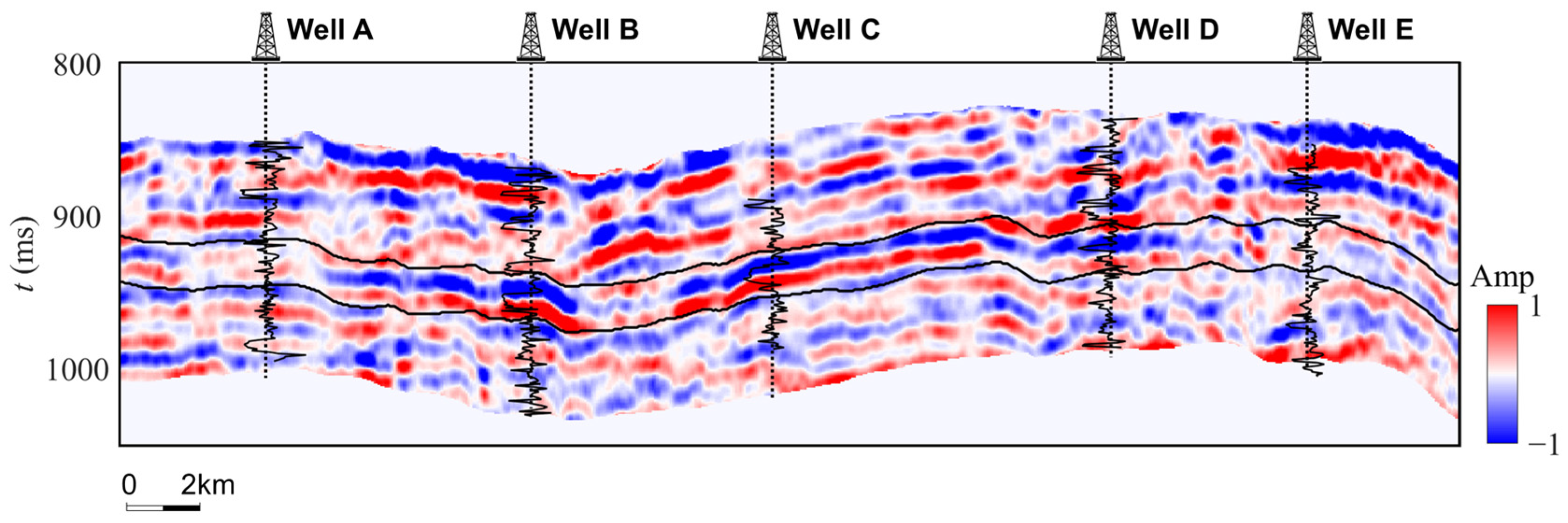
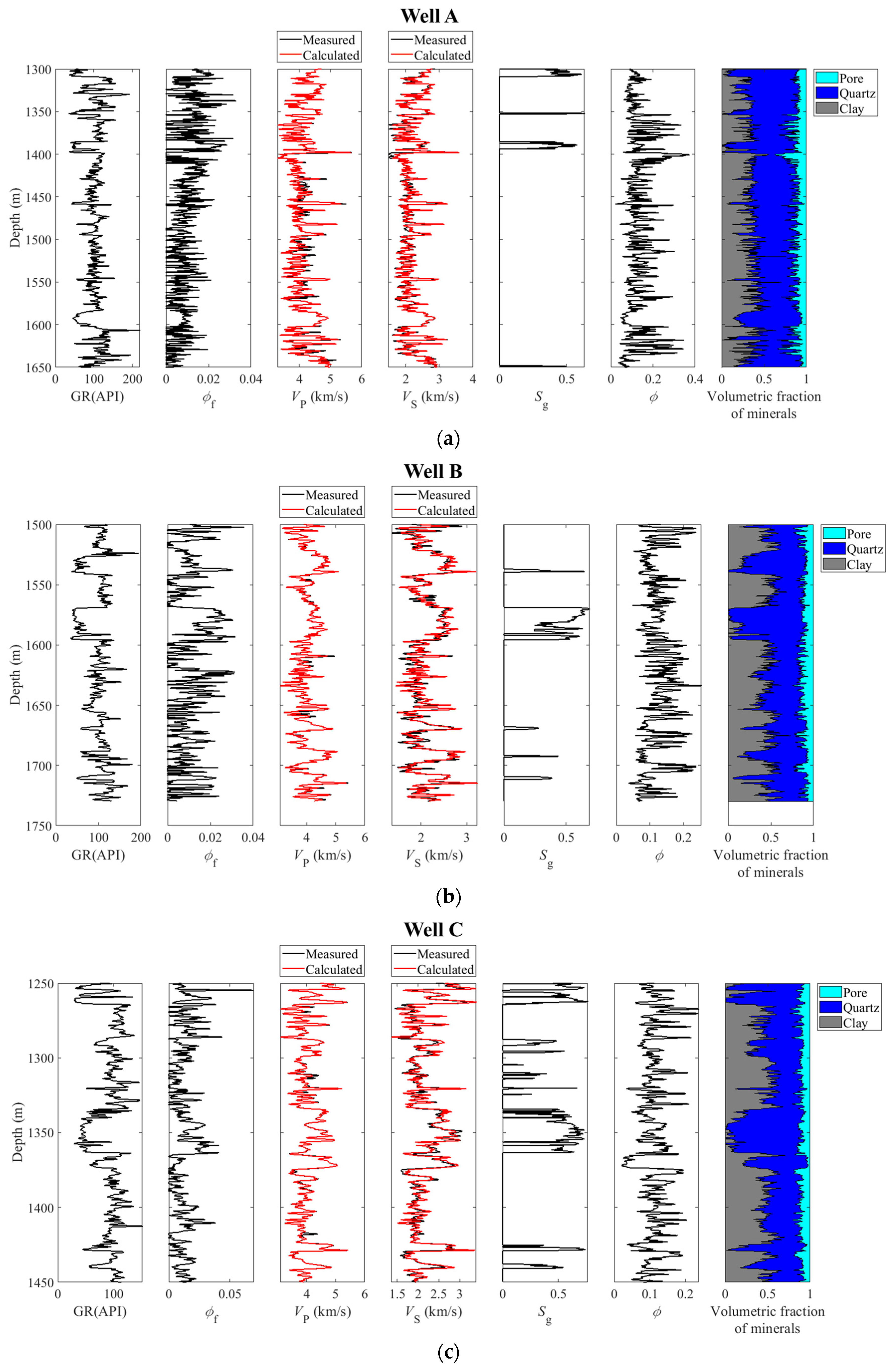
3.1. Datasets
3.2. Prediction of the Microfracture Porosity by Using the DP Model
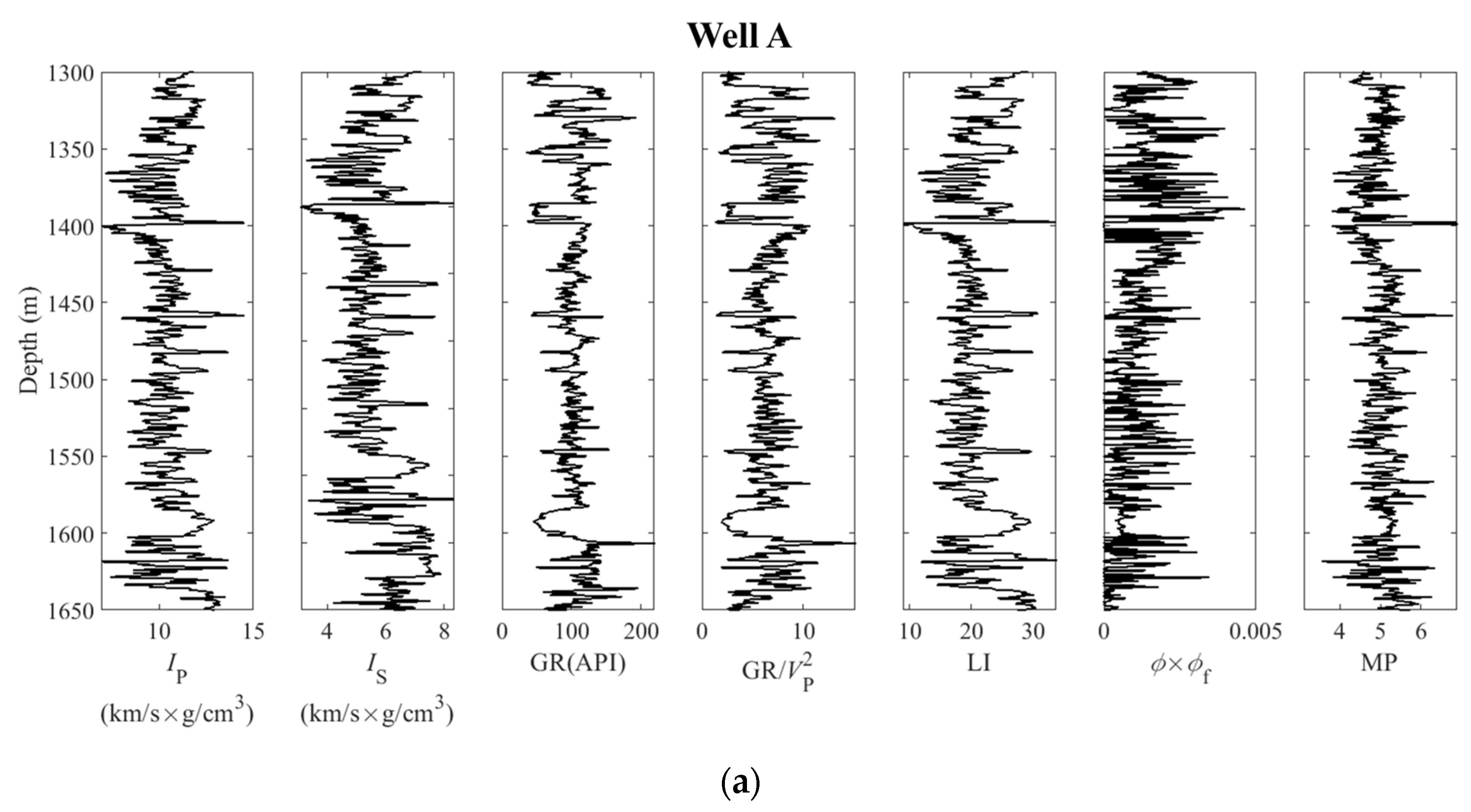
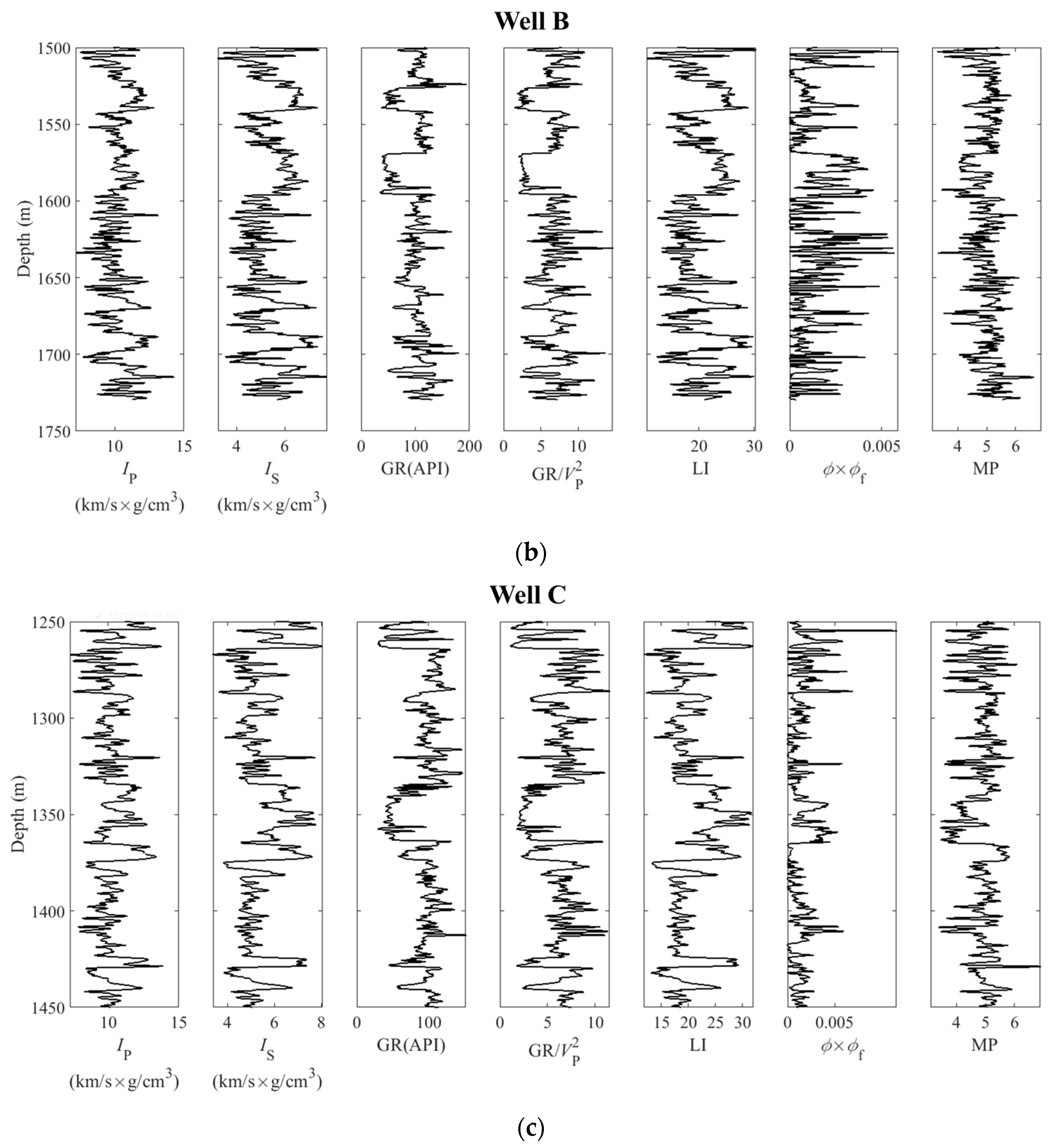
3.3. LI and MP Parameters That Are Represented by the Elastic Properties IP and IS
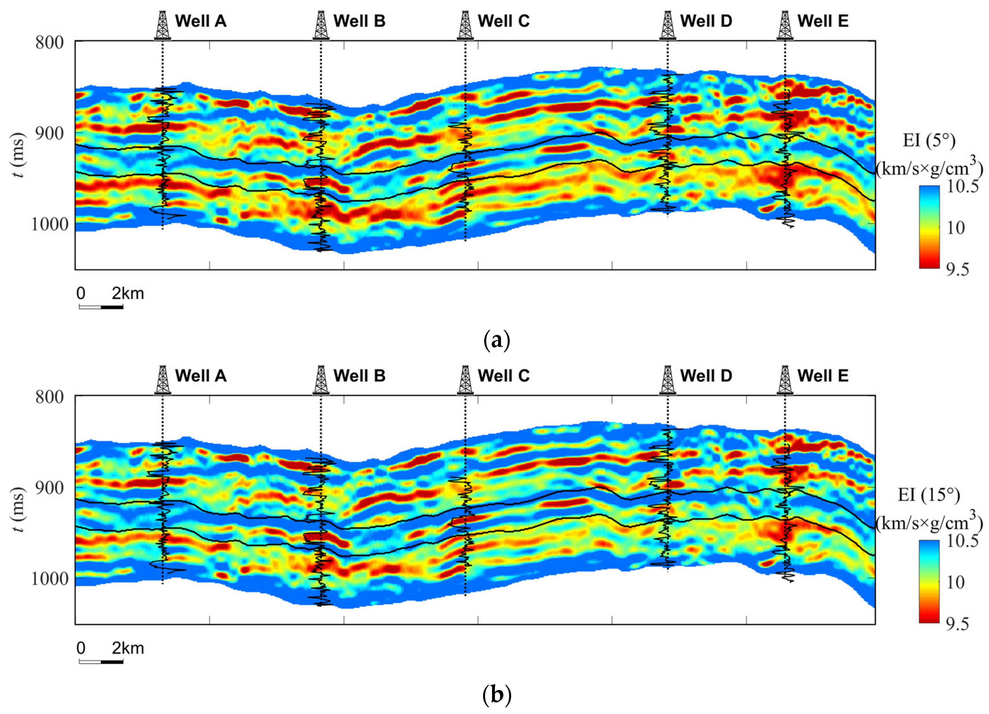
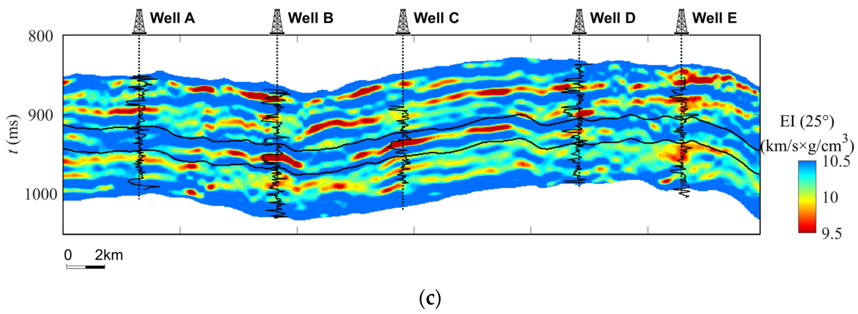
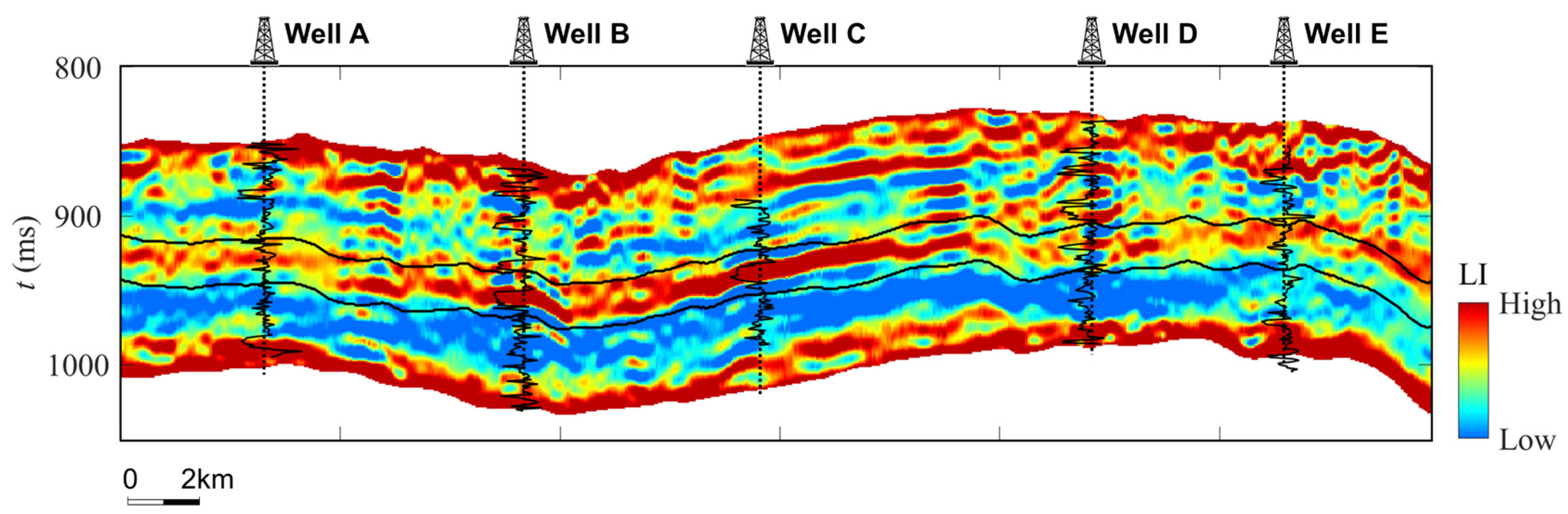
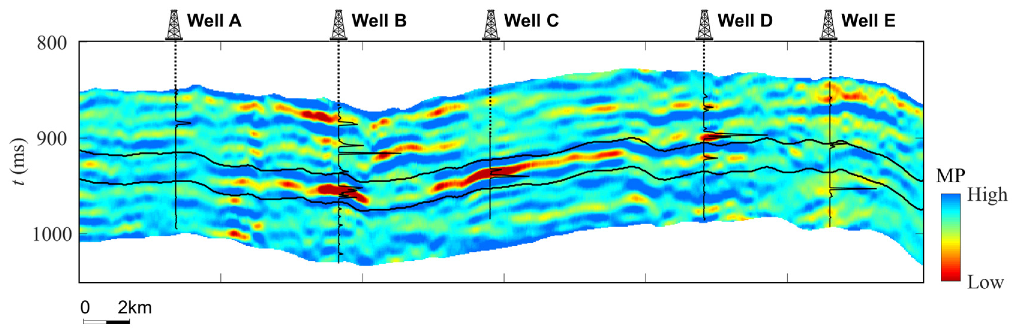
3.4. Estimation of LI and MP by Using the Proposed Elastic Impedance Inversion Method
3.5. Comprehensive Characterization of the Tight Gas Sandstone Reservoir
4. Discussion
5. Conclusions
- (1)
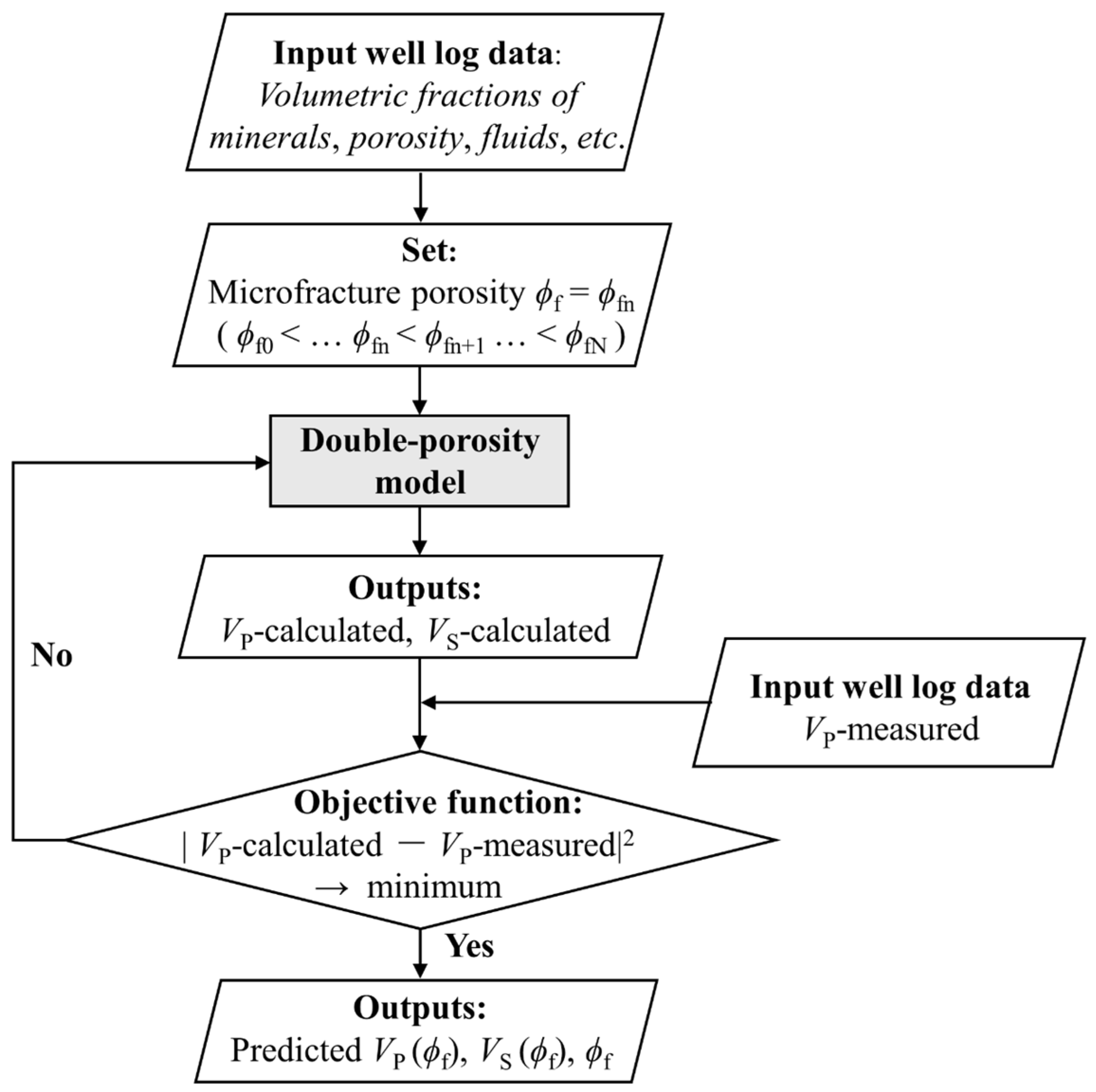
- The DP model was validated as a useful modeling tool for tight sandstones with complex pore structures. The microfracture porosity, ϕf, could be used as a practical fitting parameter when modeling the velocities of the tight sandstones and acts as a useful factor in the evaluation of microfracture development;
- (2)
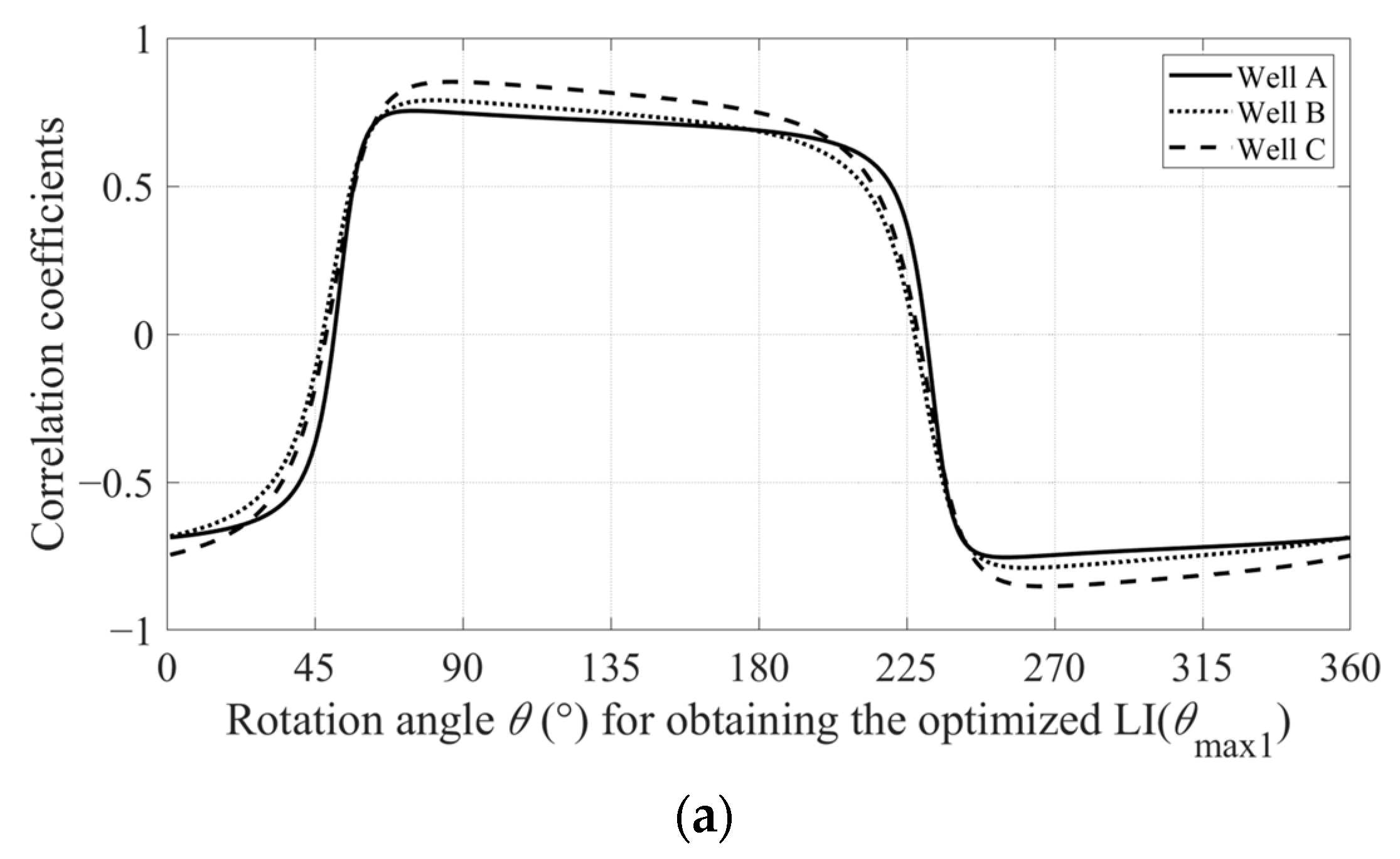
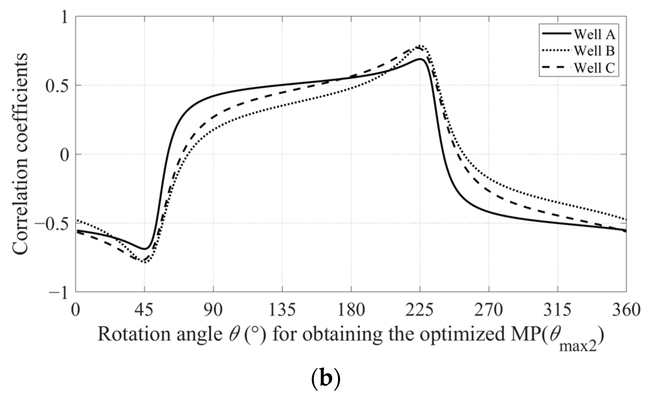
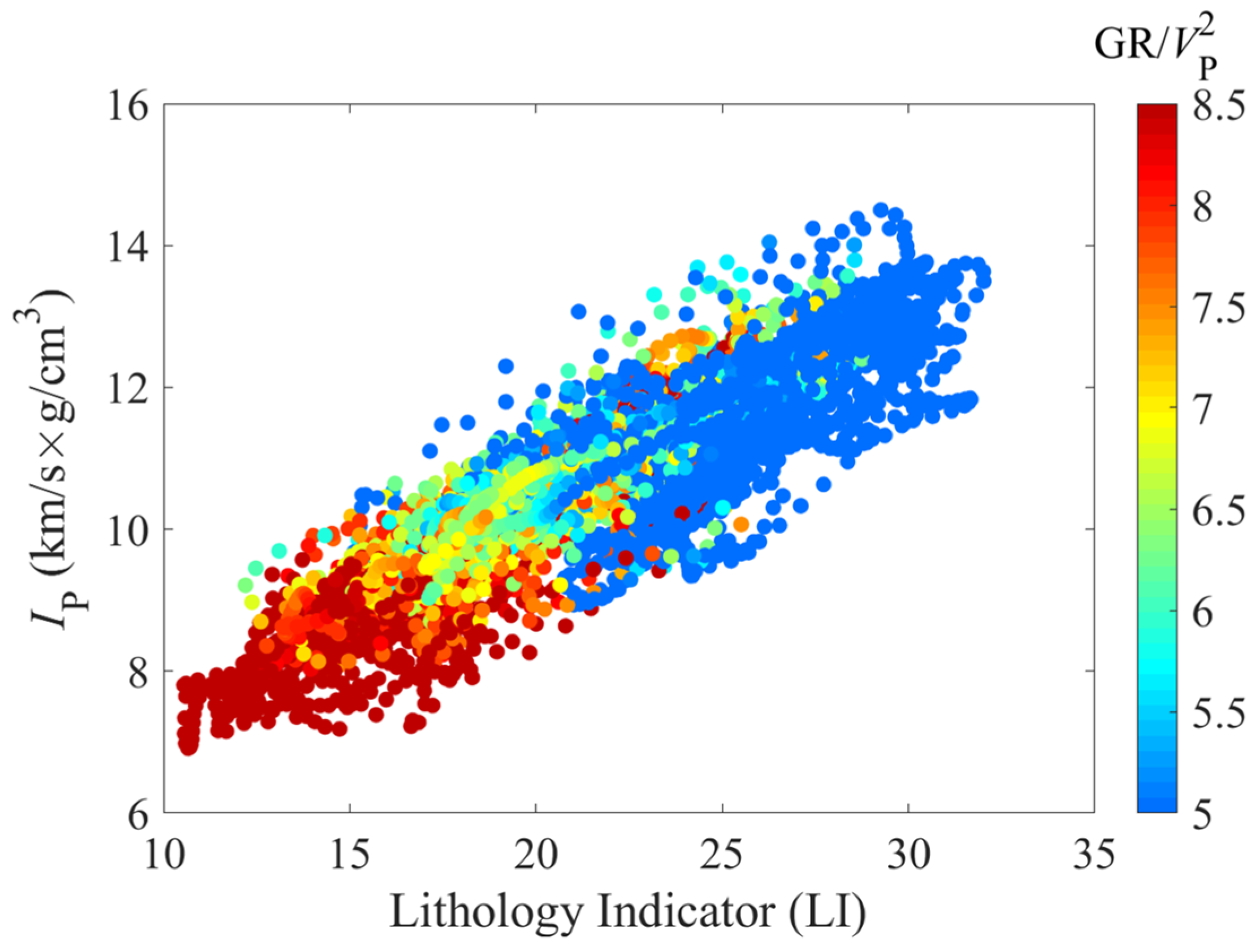
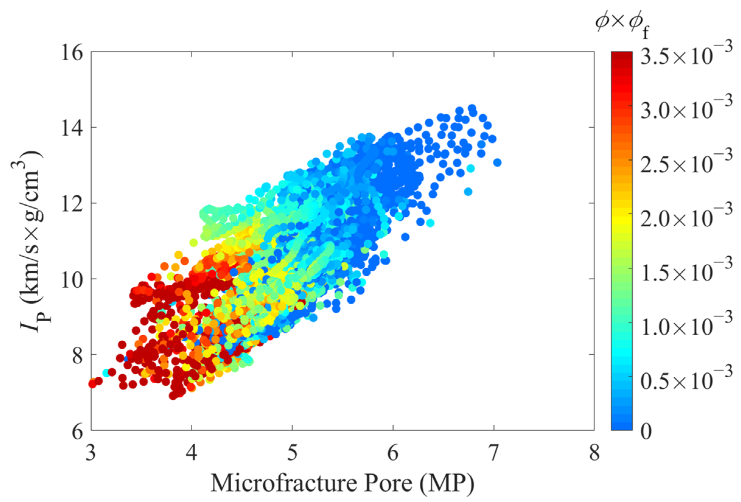
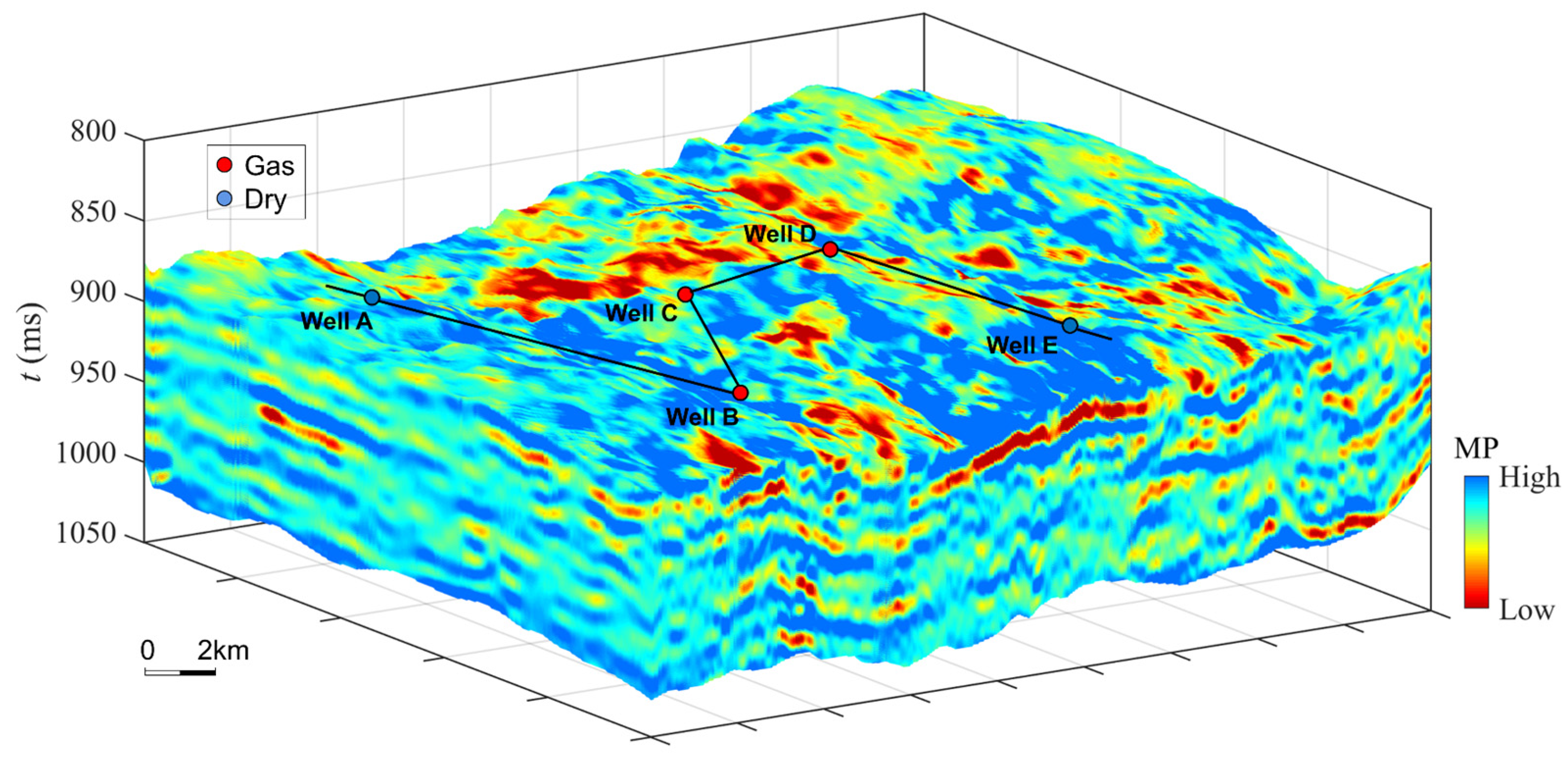
- By using the framework of the Poisson impedance, the proposed lithology indicator, LI, and the pore structure parameter, MP, were obtained from the maximum correlation between GR/VP2, ϕ × ϕf, and the elastic properties IP and IS. The LI indicator showed satisfactory performance in the discrimination of tight sandstones from mudstones. The MP indicator provided an applicable indicator for the permeable zones in tight formations;
- (3)
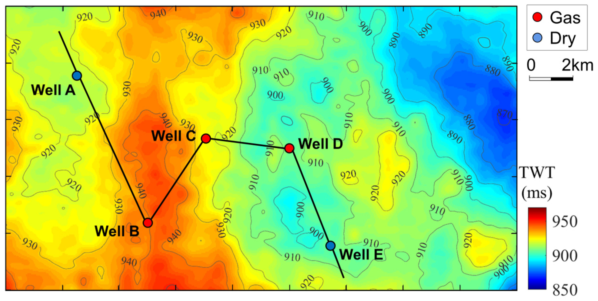
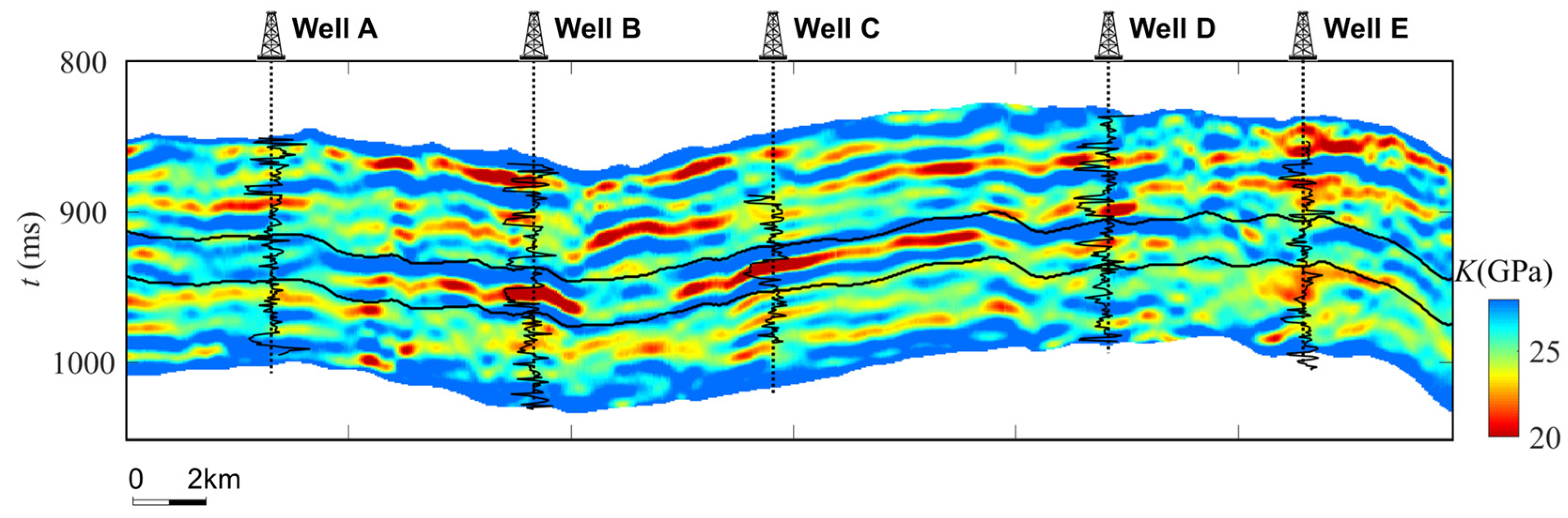
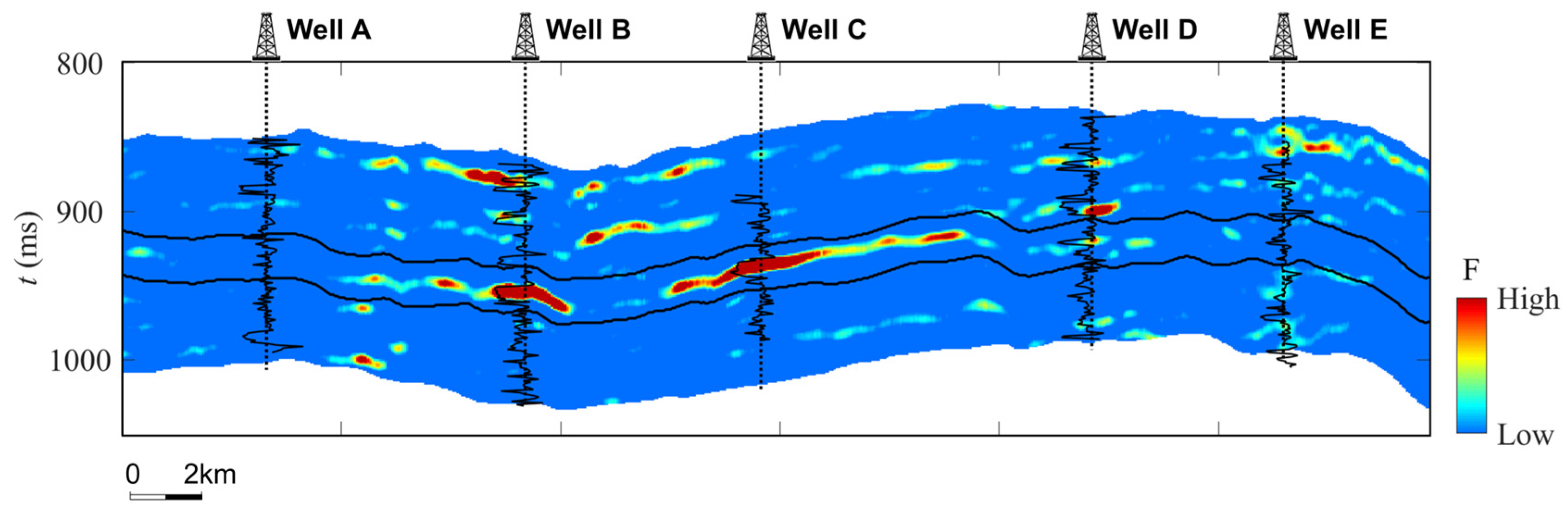
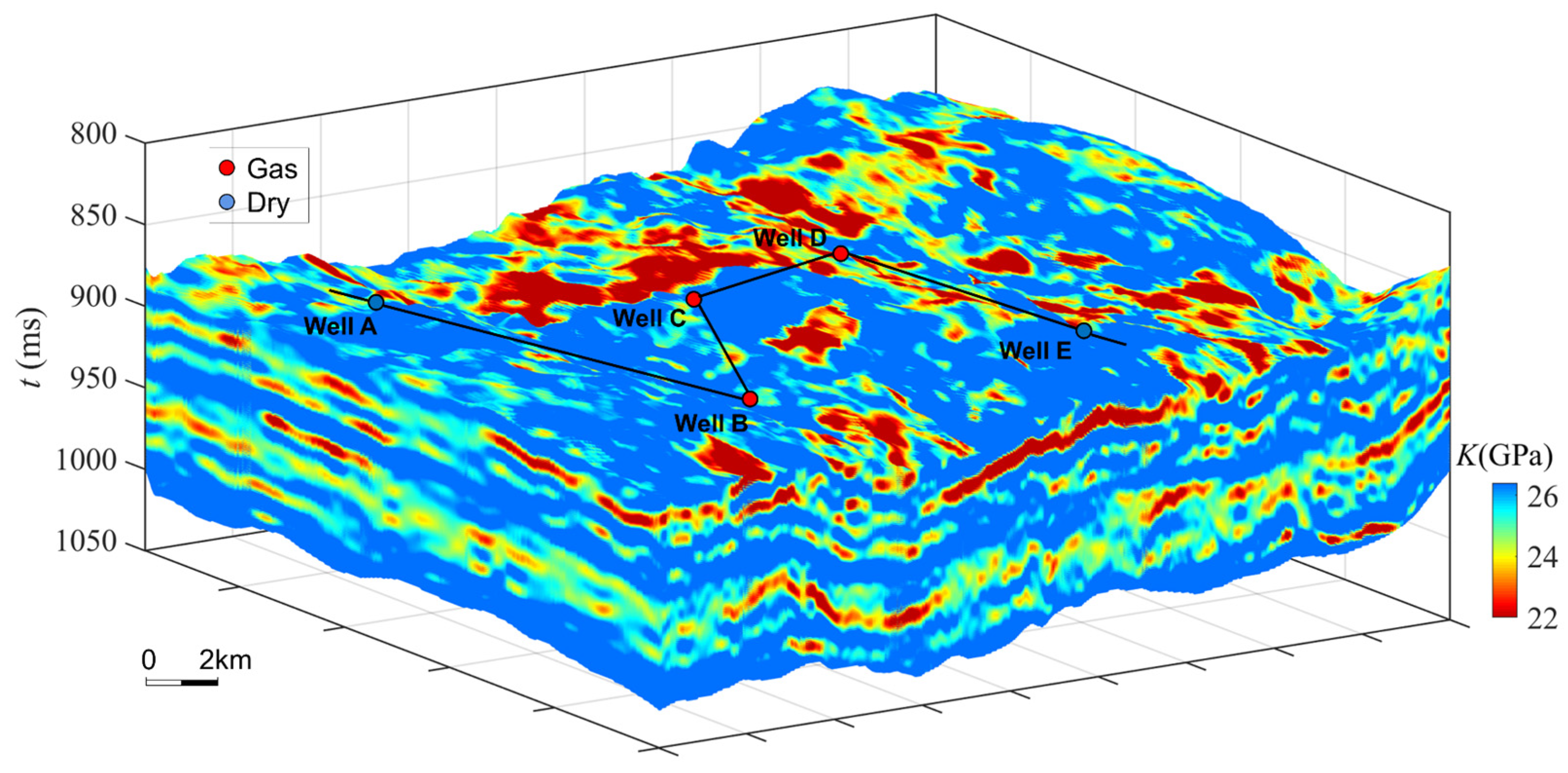
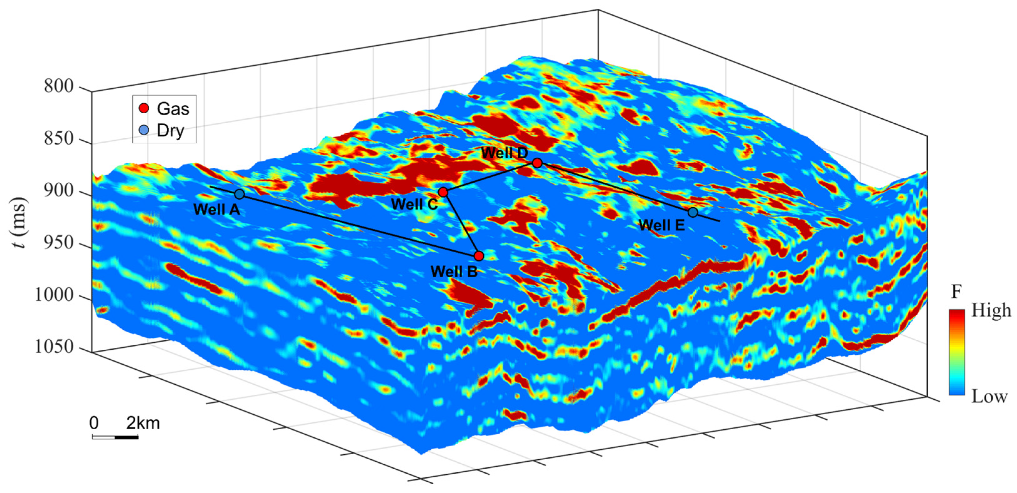
- A new AVO equation was established based on the optimized LI and MP parameters. Real data applications showed that the seismic-inverted LI and MP parameters could function as useful indicators for the optimal lithology and permeable zones in the tight gas sandstones in Ordos Basin, China. The obtained results were consistent with the measured petrophysical properties in the wellbores and agreed with the production status of the wells. Furthermore, a combined F, considering the comprehensive effects of lithology, pore structure, and gas saturation, provided a useful method for the identification of favorable areas in tight formations.
Author Contributions
Funding
Data Availability Statement
Conflicts of Interest
Appendix A
References
- Yang, H.; Liu, X.S.; Yang, Y. Status and prospects of tight gas exploration and development in the Ordos Basin. Strateg. Study CAE 2012, 14, 40–48. [Google Scholar] [CrossRef]
- Hu, C.Y.; Qian, K.; Wang, X.Q.; Shi, Z.S.; Zhang, G.W.; Xu, H.Z. Critical factors for the formation of an Upper Paleozoic giant gas field with multiple gas reservoirs in Ordos Basin and the transmutation of gas reservoir properties. Acta Petrol. Sin. 2010, 31, 879–884. [Google Scholar] [CrossRef]
- Li, X.Z.; Zhang, M.L.; Xie, W.R. Controlling factors for lithologic gas reservoir and regularity of gas distribution in the Upper Paleozoic of Ordos Basin. Acta Petrol. Sin. 2009, 30, 168–175. [Google Scholar] [CrossRef]
- Wang, D.X. A study on the rock physics model of gas reservoir in tight sandstone. Chin. J. Geophys. 2017, 60, 64–83. [Google Scholar] [CrossRef]
- Yin, H.; Zhao, J.; Tand, G.; Zhao, L.; Ma, X.; Wang, S. Pressure and fluid effect on frequency-dependent elastic moduli in fully saturated tight sandstone. Geophys. Res. Solid Earth 2017, 122, 8925–8942. [Google Scholar] [CrossRef]
- Guo, Z.Q.; Zhao, D.Y.; Liu, C. Gas prediction using an improved seismic dispersion attribute inversion for tight sandstone gas reservoirs in the Ordos Basin, China. J. Nat. Gas Sci. Eng. 2022, 101, 104499. [Google Scholar] [CrossRef]
- Guo, Z.Q.; Zhao, D.Y.; Liu, C. A New Seismic Inversion Scheme Using Fluid Dispersion Attribute for Direct Gas Identification in Tight Sandstone Reservoirs. Remote Sens. 2022, 14, 5326. [Google Scholar] [CrossRef]
- Zhang, J.; Li, X.Z.; Shen, W.J.; Gao, S.S.; Liu, H.X.; Ye, L.Y.; Fang, F.F. Study of the Effect of Movable Water Saturation on Gas Production in Tight Sandstone Gas Reservoirs. Energies 2020, 13, 4645. [Google Scholar] [CrossRef]
- Pan, X.P.; Zhang, G.Z. Amplitude variation with incident angle and azimuth inversion for Young’s impedance, Poisson’s ratio and fracture weaknesses in shale gas reservoirs. Geophys. Prosp. 2019, 67, 1898–1911. [Google Scholar] [CrossRef]
- Pan, X.P.; Zhang, P.F.; Zhang, G.Z.; Guo, Z.W.; Liu, J.X. Seismic characterization of fractured reservoirs with elastic impedance difference versus angle and azimuth: A low-frequency poroelasticity perspective. Geophysics 2021, 86, M123–M139. [Google Scholar] [CrossRef]
- Zhang, G.Z.; Yang, R.; Zhou, Y.; Li, L.; Du, B.Y. Seismic fracture characterization in tight sand reservoirs: A case study of the Xujiahe Formation, Sichuan Basin, China. Appl. Geophys. 2022, 203, 104690. [Google Scholar] [CrossRef]
- Guo, Z.Q.; Nie, N.F.; Liu, C. Fracture characterization based on improved seismic amplitude variation with azimuth inversion in tight gas sandstones, Ordos Basin, China. Mar. Pet. Geol. 2022, 146, 105941. [Google Scholar] [CrossRef]
- Liu, Y.S.; Zhu, Z.P.; Pan, R.F.; Gao, B.; Jin, J. Analysis of AVAZ Seismic Forward Modeling of Fracture-Cavity Reservoirs of the Dengying Formation, Central Sichuan Basin. Energies 2022, 15, 5022. [Google Scholar] [CrossRef]
- Smith, T.M.; Sayers, C.M.; Sondergeld, C.H. Rock properties in low-porosity/low-permeability sandstones. Lead. Edge 2009, 28, 48–59. [Google Scholar] [CrossRef]
- Ruiz, F.; Cheng, A. A rock physics model for tight gas sand. Lead. Edge 2010, 29, 1484–1489. [Google Scholar] [CrossRef]
- Sun, W.; Ba, J.; Carcione, J.M. Theory of wave propagation in partially saturated double-porosity rocks: A triple-layer patchy model. Geophys. J. Int. 2016, 205, 22–37. [Google Scholar] [CrossRef]
- Ba, J.; Xu, W.; Fu, L.; Carcione, J.M.; Zhang, L. Rock anelasticity due to patchy saturation and fabric heterogeneity: A double double-porosity model of wave propagation. Geophys. Res. Solid Earth 2017, 122, 1949–1976. [Google Scholar] [CrossRef]
- Guo, Z.Q.; Qin, X.Y.; Zhang, Y.M.; Niu, C.; Wang, D.; Ling, Y. Numerical investigation of the effect of heterogeneous pore structures on elastic properties of tight gas sandstones. Front. Earth Sci. 2021, 9, 641637. [Google Scholar] [CrossRef]
- Cheng, W.; Ba, J.; Carcione, J.M.; Pang, M.Q.; Wu, C.F. Estimation of the Pore Microstructure of Tight-Gas Sandstone Reservoirs with Seismic Data. Front. Earth Sci. 2021, 9, 646372. [Google Scholar] [CrossRef]
- Ruan, C.; Ba, J.; Carcione, J.M.; Chen, T.; He, R. Microcrack Porosity Estimation Based on Rock Physics Templates A Case Study in Sichuan Basin, China. Energies 2021, 14, 7225. [Google Scholar] [CrossRef]
- Zhou, H.T.; Li, D.Y.; Liu, X.T.; Du, Y.S.; Gong, W. Sweet spot prediction in tight sandstone reservoir based on well-bore rock physical simulation. Pet. Sci. 2019, 16, 1285–1300. [Google Scholar] [CrossRef]
- Tan, W.H.; Ba, J.; Müller, T.; Fang, G.; Zhao, H.B. Rock Physics Model of Tight Oil Siltstone for seismic prediction of brittleness. J. Geophys. Prosp. 2020, 68, 1554–1574. [Google Scholar] [CrossRef]
- Zhang, T.T.; Sun, Y.F. Two-parameter prestack seismic inversion of porosity and pore-structure parameter of fractured carbonate reservoirs: Part 1—Methods. Interpretation 2018, 6, SM1–SM8. [Google Scholar] [CrossRef]
- Zhang, T.T.; Zhang, R.F.; Tia, J.Z.; Lu, L.F.; Qin, F.Q.; Zhao, X.Z.; Sun, Y.F. Two-parameter prestack seismic inversion of porosity and pore-structure parameter of fractured carbonate reservoirs: Part 2—Applications. Interpretation 2018, 6, SM9–SM17. [Google Scholar] [CrossRef]
- Wei, Y.L.; Zhao, L.Y.; Liu, W.; Zhang, X.; Guo, Z.J.; Wu, Z.L.; Yuan, S.H. Coalbed Methane Reservoir Parameter Prediction and Sweet-Spot Comprehensive Evaluation Based on 3D Seismic Exploration: A Case Study in Western Guizhou Province, China. Energies 2022, 16, 367. [Google Scholar] [CrossRef]
- Aleardi, M. Estimating petrophysical reservoir properties through extended elastic impedance inversion: Applications to off-shore and on-shore reflection seismic data. J. Geophy. Eng. 2018, 15, 2079–2090. [Google Scholar] [CrossRef]
- Zhang, F.C.; Yang, J.Y.; Li, C.H.; Li, D.; Gao, Y. Direct inversion for reservoir parameters from prestack seismic data. J. Geophy. Eng. 2020, 17, 993–1004. [Google Scholar] [CrossRef]
- Guo, Z.Q.; Qin, X.Y.; Liu, C. Pore and microfracture characterization in tight gas sandstone reservoirs with a new rock-physics-based seismic attribute. Remote Sens. 2023, 15, 289. [Google Scholar] [CrossRef]
- Li, X.Y.; Wang, J.C.; Zhao, D.D.; Ni, J.; Lin, Y.P.; Zhang, A.G.; Zhao, L.; Liu, Y.M. Quantitative Evaluation of Water-Flooded Zone in a Sandstone Reservoir with Complex Porosity-Permeability Relationship Based on J-Function Classification: A Case Study of Kalamkas Oilfield. Energies 2022, 15, 7037. [Google Scholar] [CrossRef]
- Hashin, Z.; Shtrikman, S. A variational approach to the theory of the elastic behaviour of multiphase materials. Mech. Phys. Solids 1963, 11, 127–140. [Google Scholar] [CrossRef]
- Berryman, J.G. Long-wavelength propagation in composite elastic media II. Ellipsoidal inclusions. J. Acoust. Soc. Am. 1980, 68, 1820–1831. [Google Scholar] [CrossRef]
- Quakenbush, M.; Shang, B.; Tuttle, C. Poisson impedance. Lead. Edge 2006, 25, 128–138. [Google Scholar] [CrossRef]
- Fatti, J.L.; Smith, G.C.; Vail, P.J.; Strauss, P.J.; Levitt, P.R. Detection of gas in sandstone reservoirs using AVO analysis: A 3-D seismic case history using the Geostack technique. Geophysics 1994, 59, 1362–1376. [Google Scholar] [CrossRef]
- Connolly, P. Elastic impedance. Lead. Edge 1999, 18, 438–452. [Google Scholar] [CrossRef]
- Whitcombe, D.N. Elastic impedance normalization. Geophysics 2002, 67, 60–62. [Google Scholar] [CrossRef]
- Yang, H.; Wang, D.; Zhang, M.; Wang, Y.; Liu, L.; Zhang, M. Seismic prediction method of pore fluid in tight gas reservoirs, Ordos Basin, NW China. Pet. Explor. Dev. 2017, 44, 544–551. [Google Scholar] [CrossRef]
- Fan, X.; Zhang, G.; Zhang, J. Prediction method of pore structure parameters oftight sandstone. In SEG Technical Program Expanded Abstracts 2019; Society of Exploration Geophysicists: Houston, TX, USA, 2019. [Google Scholar]
- Li, H.B.; Zhang, J.J.; Pan, H.J.; Gao, Q. Nonlinear simultaneous inversion of porestructure and physical parameters based on elastic impedance. Sci. China Earth Sci. 2021, 64, 977–991. [Google Scholar] [CrossRef]
- Cui, H.; Zhong, N.; Li, J.; Wang, D.; Li, Z.; Hao, A.; Liang, F. Study on the lower limits of petrophysical parameters of the Upper Paleozoic tight sandstone gas reservoirs in the Ordos Basin, China. J. Nat. Gas Geosci. 2017, 2, 21–28. [Google Scholar] [CrossRef]
- Ren, J.; Zhang, L.; Ezekiel, J.; Ren, S.; Meng, S. Reservoir characteristics and productivity analysis of tight sand gas in Upper Paleozoic Ordos Basin China. J. Nat. Gas Sci. Eng. 2014, 19, 244–250. [Google Scholar] [CrossRef]
- Domenico, S.N. Elastic properties of unconsolidated porous sand reservoirs. Geophysics 1977, 42, 1339–1368. [Google Scholar] [CrossRef]


Disclaimer/Publisher’s Note: The statements, opinions and data contained in all publications are solely those of the individual author(s) and contributor(s) and not of MDPI and/or the editor(s). MDPI and/or the editor(s) disclaim responsibility for any injury to people or property resulting from any ideas, methods, instructions or products referred to in the content. |
© 2023 by the authors. Licensee MDPI, Basel, Switzerland. This article is an open access article distributed under the terms and conditions of the Creative Commons Attribution (CC BY) license (https://creativecommons.org/licenses/by/4.0/).
Share and Cite
Jin, H.; Liu, C.; Guo, Z. Characterization of Tight Gas Sandstone Properties Based on Rock Physical Modeling and Seismic Inversion Methods. Energies 2023, 16, 7642. https://doi.org/10.3390/en16227642
Jin H, Liu C, Guo Z. Characterization of Tight Gas Sandstone Properties Based on Rock Physical Modeling and Seismic Inversion Methods. Energies. 2023; 16(22):7642. https://doi.org/10.3390/en16227642
Chicago/Turabian StyleJin, Han, Cai Liu, and Zhiqi Guo. 2023. "Characterization of Tight Gas Sandstone Properties Based on Rock Physical Modeling and Seismic Inversion Methods" Energies 16, no. 22: 7642. https://doi.org/10.3390/en16227642