Article

Geophysical Interpretation of Horizontal Fractures in Shale Oil Reservoirs Using Rock Physical and Seismic Methods

College of Geoexploration Science and Technology, Jilin University, Changchun 130021, China
*
Author to whom correspondence should be addressed.
Energies 2023, 16(22), 7514; https://doi.org/10.3390/en16227514
Submission received: 7 October 2023 / Revised: 3 November 2023 / Accepted: 7 November 2023 / Published: 9 November 2023
(This article belongs to the Special Issue New Challenges in Unconventional Oil and Gas Reservoirs)

Abstract

:
Horizontal fractures are one of the factors that significantly affect the ultimate productivity of shale oil reservoirs. However, the prediction of horizontal fractures by using seismic methods remains a challenge, which is due to the complex elastic and seismic responses that are associated with horizontal fractures. A framework that predicts horizontal fractures by seismic rock physical methods has been developed in the present study. A shale model is then proposed to quantify the shale elastic responses that are associated with the properties of the horizontal fractures. The modeling results that are based on the logging data validated the applicability of the proposed model, and the predicted fracture properties could be used to evaluate the development of horizontal fractures. According to the framework of the Poisson impedance, a horizontal fracture indicator is suggested to represent the logging-derived fracture density in terms of a combination of elastic properties. By using seismic-inverted elastic properties, the obtained indicator enabled an estimation of zones with the potential development of horizontal fractures. The established indicator showed a good correlation with the fracture density and could be used as an effective indicator in the prediction of horizontal fractures in shale oil reservoirs. Furthermore, seismic data applications show a consistency between the development of horizontal fractures and the production status of the boreholes. This result highlights the importance of horizontal fractures for the ultimate productivity and emphasizes the applicability of the proposed methods.

1. Introduction

As groundbreaking unconventional resources, the shale reservoirs are providing an ever-increasing amount of oil and gas around the world, and better understanding of shale microstructures will provide improved characterization of various shale reservoirs [1,2,3,4]. Successful predictions of sweet spots in shale reservoirs should consider areas that include an abundance of organic enrichments. These enrichments are indicated by various factors, such as the total organic carbon (TOC), the high brittleness of the shale rock that facilitates hydraulic fracturing, and the development of natural fractures.
Seismic methods have contributed to the characterization of such factors in shale reservoirs. By using logging data and seismic-inverted elastic properties, the TOC in the shale has been evaluated by its elastic properties. A low density or an elastic impedance usually corresponds to a high TOC [5,6,7,8,9]. Also, the brittleness of the shale rock has been estimated by its mechanical properties, such as Young’s modulus and Poisson’s ratio [10,11,12,13]. Other practical brittleness factors have also been suggested, which were based on the combination of mechanical properties and the Lamé coefficients derived from elastic properties [14,15]. In addition, vertical fractures that were associated with tectonic activities could be predicted by using various azimuthal seismic inversion methods based on the anisotropic shale model [16,17,18,19,20,21,22,23].
In particular, shale exhibits an intrinsic anisotropy that is represented as vertical transverse isotropy (VTI). It results from the anisotropy of clay particles, laminated microstructural fabrics, and layered distributions of minerals and organic matter [24,25,26,27,28,29,30]. Moreover, the horizontal fractures that are developed in the shale rock can further enhance the degree of VTI anisotropy of the shale. Early experimental investigations have shown that the opening and closing of the aligned fractures in the shale at different stresses can lead to variations in the anisotropy [31,32]. Recent experiments and core and outcrop observations have indicated that the presence of horizontal fractures in the shale can cause substantial anisotropy variations with loading stresses [33,34,35]. Geological studies have also confirmed the importance of horizontal fractures for sweet spot predictions in shale reservoirs [36,37,38,39]. Accordingly, some efforts have been made to predict the VTI anisotropy of the shale based on rock physical modeling using logging data [40]. Furthermore, seismic dispersion attributes were derived by using the frequency-dependent pre-stack seismic inversion method in the prediction of fluid-saturated bedding-parallel fractures [41]. Despite such efforts, it remains a challenge to predict horizontal fractures in the shale, which is due to the complex elastic and seismic responses of the bedding-aligned fractures.
Rock physical modeling can unravel the elastic characteristics of the shale, which are associated with various petrophysical properties. So far, numerous modeling methods have been developed to quantify the elastic responses and the corresponding seismic signatures of organic matter in the shale [14,24,27,28,29,32,42,43,44,45]. In addition, the shale anisotropy that is related to clay lamination and microstructural fabrics has been investigated by using modeling methods [43,46,47]. The shale brittleness has also been incorporated in the rock physical modeling for the prediction of engineering sweet spots in shale reservoirs [9,48]. However, shale models that quantify the effect of horizontal fractures on the shale elastic properties are rare. Further investigations are, therefore, needed to develop practical methods with which it is possible to predict horizontal fractures from logging data, in addition to seismic data that are based on the shale model.
In the present study, rock physical modeling and seismic methods are developed for the prediction of horizontal fractures in shale oil reservoirs. At first, a shale model is proposed for the description of elastic responses associated with horizontal fracture properties. As the next step, various horizontal fracture properties are estimated by using logging data and the established shale model. Based on the framework of the Poisson impedance, a horizontal fracture indicator is, thereafter, proposed to represent the logging-derived fracture density in terms of elastic properties. The obtained indicator is then applied to seismic data from a shale oil reservoir for a quantitative interpretation of the horizontal fractures from seismic-inverted elastic properties. Finally, the calculated results are compared with TOC and validated with the production status of the boreholes in the studied areas.

2. Methods

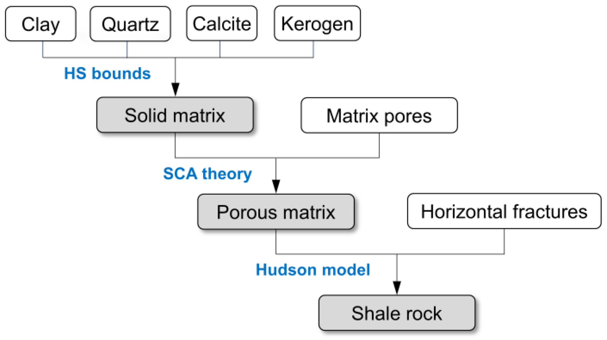
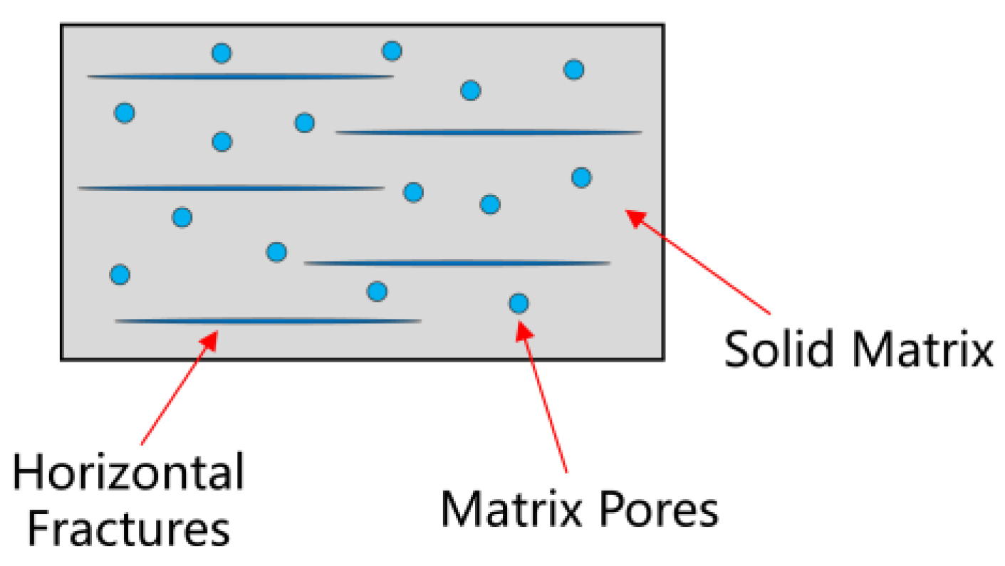
2.1. Rock Physics Model of Shale Oil Reservoirs

As shown in Figure 1, a framework for the modeling of shales has been proposed for the quantification of the effect of horizontal fractures on the shale elastic properties. At first, the theory of Hashin-Shtrikman (HS) bounds [49] was used to calculate equivalent elastic moduli of the shale solid matrix. According to the core analyses, the shale matrix is mainly composed of clay, quartz, calcite, and kerogen. In the modeling, the organic kerogen material was treated as a part of the solid matrix. Furthermore, the elastic moduli of the porous shale matrix were obtained by using the self-consistent approximation (SCA) theory [50], which considered the effect of fluid-filled matrix pores. Finally, the Hudson model [51] was used to add fluid-filled horizontal fractures to the porous matrix to obtain elastic properties of the shale rock. Specifically, in the proposed modeling method, the total porosity (ϕ) was considered as pore spaces that consisted of matrix pores (ϕm) and horizontal fractures (ϕf) (Figure 2). In addition, fluid mixtures of water and oil were assumed to be homogeneously distributed in the matrix pores and horizontal fractures [52]. The rock physical theories that were used in the modeling are described in the following sections.

2.2. Hashin-Shtrikman Bounds

Hashin and Shtrikman (1963) [49] proposed a method to predict the equivalent elastic moduli of a mixture of mineral particles (Equation (1)):
K H S ± = K 1 + f 2 ( K 2 K 1 ) 1 + f 1 ( K 1 + 4 3 μ 1 ) 1 μ H S ± = μ 1 + f 2 ( μ 2 μ 1 ) 1 + 2 f 1 ( K 1 + 2 μ 1 ) 5 μ 1 ( K 1 + 4 3 μ 1 )
where K H S ± and μ H S ± represent the narrowest upper and lower limits of bulk and shear modulus of the mixture consisting of two or more mineral phases, respectively. Ki and μi represent the bulk and shear moduli, respectively, of each component. Also, fi is the volume fraction component.
When the mixture has more than two types of mineral particles, the equivalent elastic moduli could be expressed in a general form (Equation (2)):
K H S + = Λ ( μ max ) , K H S = Λ ( μ min ) μ H S + = Γ ζ ( K max , μ max ) , μ H S = Γ ζ ( K min , μ min )
where
Λ ( z ) = 1 K ( r ) + 4 3 z 4 3 z Γ ( z ) = 1 μ ( r ) + z 1 z ζ ( K , μ ) = μ 6 ( 9 K + 8 μ K + 2 μ )
where K(r) and μ(r) represent the bulk and shear modulus corresponding to the r’th component of the solid matrix; z represents the corresponding argument in Equation (2). The <·> bracket denotes the volumetric average of each component.

2.3. Self-Consistent Approximation Theory

Berryman (1980) [50] presented the SCA theory for an equivalent medium. A method was presented to calculate the elastic moduli of a model composed of multiphase minerals and pore spaces. The corresponding equations were represented in Equation (4):
i = 1 N x i ( K i K S C * ) P * i = 0 i = 1 N x i ( μ i μ S C * ) Q * i = 0
where K S C * and μ S C * are the equivalent bulk and shear modulus of the entire rock, respectively. The subscript i represents each mineral phase or pore space, and xi represents the volume fraction of each phase. Also, Ki and μi represent the bulk modulus and shear modulus, respectively, for each phase. The superscript *i of P and Q is the geometric factor for the inclusion material i. Furthermore, the coefficients P*i and Q*i represent the geometries of the inclusions.

2.4. Hudson Model

Hudson (1981) [51] established a penny-shaped microfracture model for the calculations of stiffness coefficients for a rock embedded with parallel microfractures (Equation (5)):
c i j = c i j 0 + c i j 1
where c i j 0 represents the elastic stiffness matrix of the host medium, and c i j 1 represents the first-order disturbances by the microfractures. The corresponding equations were presented in Equation (6):
c 11 1 = λ 2 μ ε f U 3 c 13 1 = λ ( λ + 2 μ ) μ ε f U 3 c 33 1 = λ ( λ + 2 μ ) 2 μ ε f U 3 c 44 1 = μ ε f U 1 c 66 1 = 0
where λ and μ represent the Lamé constants of the host medium. Also, U1 and U3 depend on the states of the microfractures, and εf is the fracture density (Equation (7)):
ε f = 3 ϕ f 4 π α
where ϕf and α represent the fracture porosity and the aspect ratio, respectively.
The definitions of the fluid-filled fractures were presented in Equation (8):
U 3 = 4 ( λ + 2 μ ) 3 ( λ + μ ) 1 1 + κ U 1 = 16 ( λ + 2 μ ) 3 ( 3 λ + 4 μ )
where κ is the parameter that is used to describe the fracture characteristics (Equation (9)):
κ = K f ( λ + 2 μ ) π α μ ( λ + μ )
where Kf represents the fluid bulk modulus.

2.5. Domenico Equation for the Fluid Mixture

Domenico (1977) [52] proposed a method for calculations of the bulk moduli of fluid mixtures. In the modeling of the shale oil reservoirs in our paper, the fluids were assumed to be a mixture of oil and water, homogeneously distributed in the spaces of matrix pores and horizontal fractures. The modulus of the mixed fluid was estimated by using Equation (10):
K f = S w K w + S o K o
where Kw and Ko represent the moduli of water and oil, respectively, and the corresponding saturations of water and oil are represented by Sw and So, respectively.
Also, the density of the mixed fluid was calculated by using Equation (11):
ρ f = S w ρ w + S o ρ o
where ρw and ρo represent water and oil density, respectively.

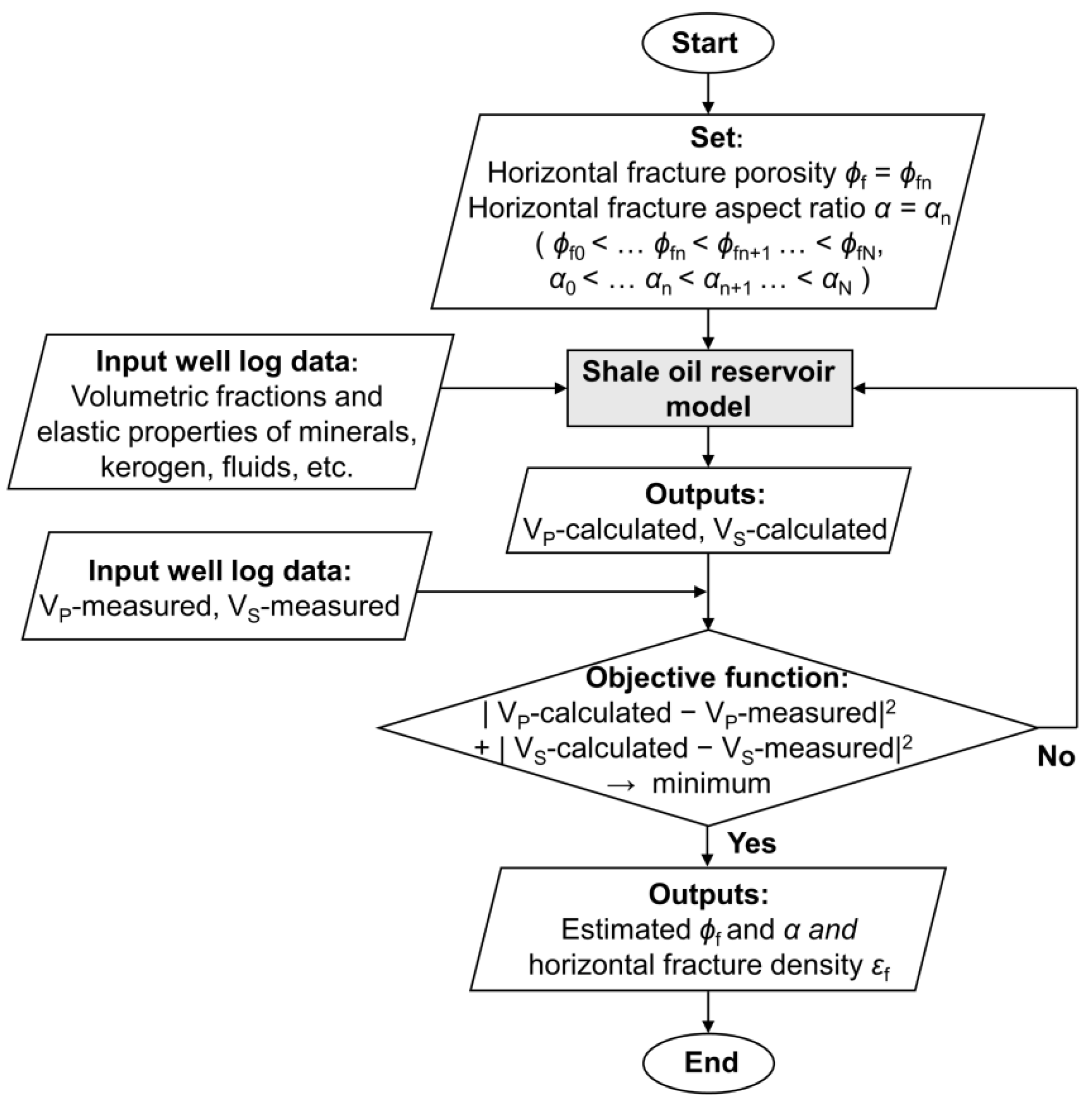
2.6. Prediction of the Horizontal Fracture Properties by Using the Shale Model and Logging Data

The proposed model for the shale oil reservoir (Figure 1) was used to develop a method for the estimation of horizontal fractures based on a model-based framework. By using well-log data, the shale model acted as a modeling tool in the prediction of the horizontal fracture density, εf (Figure 2). Specifically, the volumetric fractions and moduli of the minerals, kerogen, and fluids were as input data for modeling P-wave and S-wave velocities (i.e., VP-calculated and VS-calculated) for a set of preset values of horizontal fracture porosities (ϕf) and aspect ratios (α). An objective function (Equation (12)) was, thereafter, constructed to find the optimized values of (ϕf, α) by minimizing the difference between VP-calculated and VS-calculated and the corresponding measured values (i.e., VP-measured and VS-measured) in the borehole:
f ϕ f , α = min V P calculated ϕ f , α V P measured 2 + V S calculated ϕ f , α V S measured 2
Based on Equation (12), a simple grid-searching method has in the present study been used to find the optimized values of ϕf and α. According to Equation (7), the estimated ϕf and α values were finally used to compute the fracture density, εf.

2.7. Estimation of the Horizontal Fracture (HF) Indicator from Elastic Properties

For the characterization of horizontal fractures by using seismic data, it is essential to find an applicable seismic attribute that correlates with the fracture density, εf, estimated by using the method presented in Figure 3. Based on the framework of the Poisson impedance [53,54,55], a horizontal fracture (HF) indicator was then proposed, as represented by seismic attributes in Equation (13):
HF θ = I P cos θ V P / V S sin θ
where θ represents the rotation angle that transforms the P-wave impedance (IP) and P-to-S-wave velocity ratio (VP/VS) to HF.
Then, the maximum correlation between HF(θ) (as represented by Equation (13)) and εf (as predicted from well-log data) was determined by optimizing the θmax value. By using the seismic-derived elastic properties, the obtained HF(θmax) was, thereafter, used to estimate the horizontal fractures in the shale oil reservoirs.

3. Results

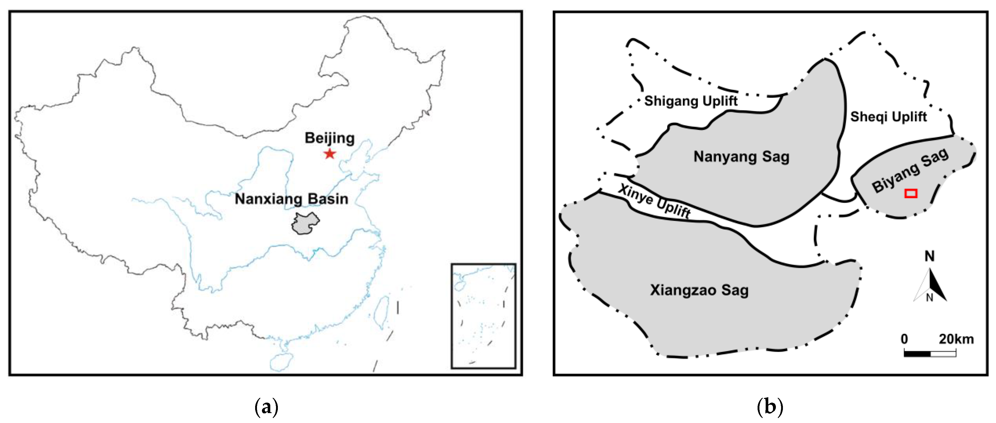
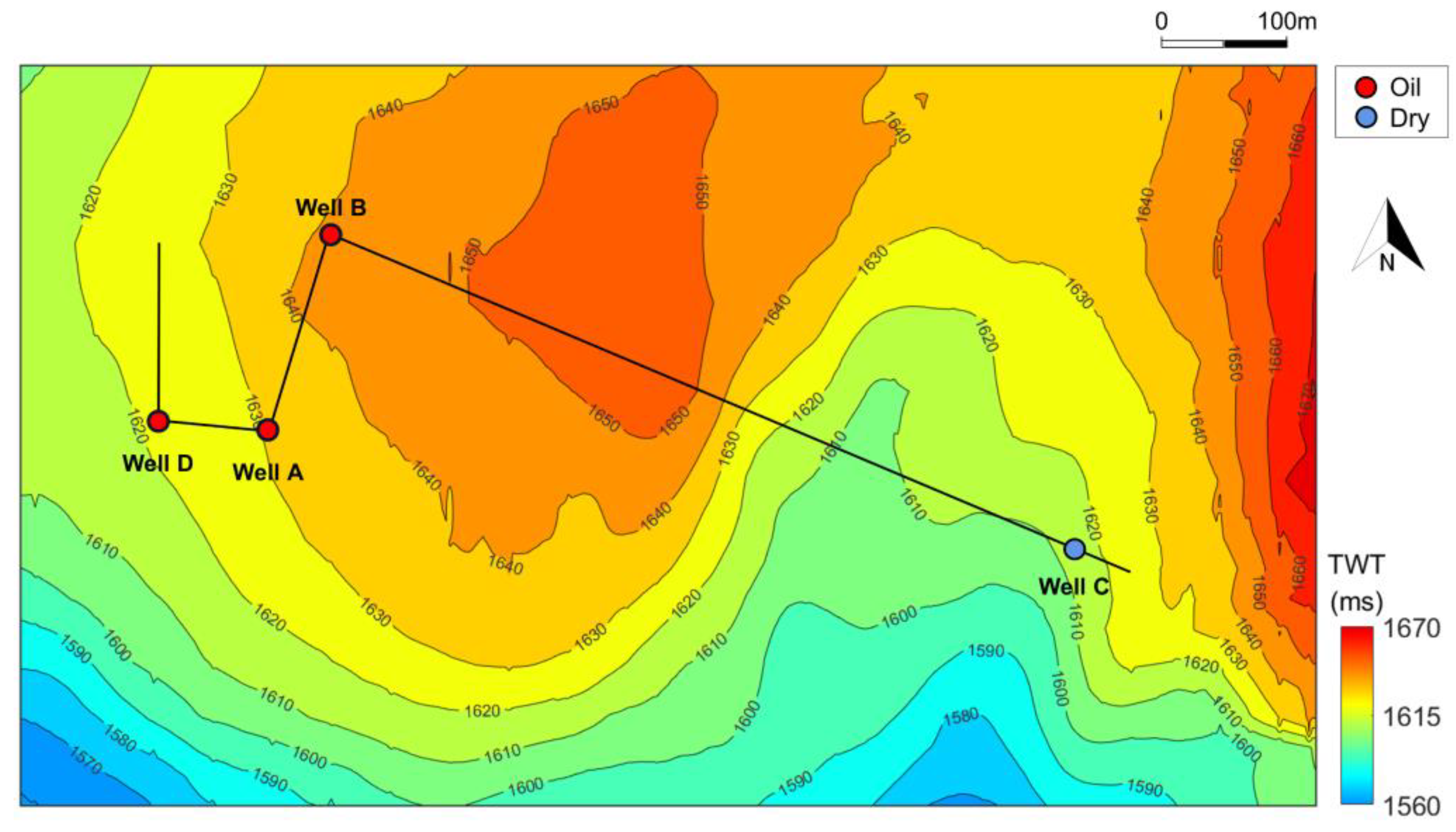
3.1. Studied Area and Datasets

As can be seen in Figure 4a, the Nanxiang Basin is located in the middle south of China. Biyang Sag is a secondary structural unit of the Nanxiang Basin, which is located northeast of the Nanxiang Basin (Figure 4b). In the present study, the studied area of the shale oil reservoirs is located in the lower middle of the Biyang Sag, as denoted by the red box in Figure 4b. Also, Figure 5 illustrates the stratigraphic units and sedimentary facies in the studied area. For the studied area, the Taicangfang-Yuhuangding, Hetaoyuan, and Liaozhuang formations have been developed in the Paleogene, while the Shangsi formation has been developed in the Neogene in the studied area. The deposition period of the Hetaoyuan formation in the Biyang Sag overlaps with the peak period of the lacustrine basin development, and the sedimentary facies are characterized by shallow to deep lacustrine facies. The shale is mainly developed in the second (Eh2) and third (Eh3) members of the Hetaoyuan formation, and the Eh3 is the main oil-bearing layer in the Biyang Sag. There are six sets of organic material-rich intervals (ORI), as indicated by 1-6 from top to bottom, in the Eh3. Out of these, the ORI 5 is a great organic enrichment layer with a large cumulative thickness and a high total organic content. It shows a good shale oil resource potential as the main exploration target reservoir [56,57].
The seismic data were obtained by a three-dimensional seismic acquisition in the studied area. As can be seen in Figure 6, the map of the seismic two-way time for the target shale oil reservoir showed that the geological structure of the target layer was relatively smooth. The positions of the oil wells (A, B, and D) and the dry well (C), as well as the seismic lines across these wells, are illustrated in Figure 6. Among these, wells A, B, and C are vertical wellbores, while well D has a range of horizontal trajectories. Furthermore, Figure 7 shows the seismic profile where the horizons of the target shale oil layer are indicated. The bottom line in Figure 7 illustrates the bottom limit selected for seismic inversion of elastic parameters and the estimation of HF accordingly. For the studied area, the three-dimensional data volumes of the elastic properties were obtained by a pre-stack seismic inversion.
The measured logging curves for well A are displayed in Figure 8, where the interval of the target shale is especially indicated. The target shale layer had a medium porosity (ϕ) and relatively high oil saturation (So). According to the geological analyses of the studied region, the horizontal fractures were supposed to contribute to the reservoir permeability and affect the ultimate production. As shown in Figure 9, the formation micro-scanner image (FMI) for well A indicated the presence of horizontal fractures in the target shale layer (as indicated by green and blue lines). It is, therefore, important to estimate the horizontal fractures by using shale modeling and logging data and to predict the horizontal fracture distributions by using seismic-inverted elastic properties. Accordingly, rock physical modeling has been performed based on the logging data from well A. The horizontal fractures were then estimated, followed by the establishment of a correlation between the horizontal fractures and elastic properties.

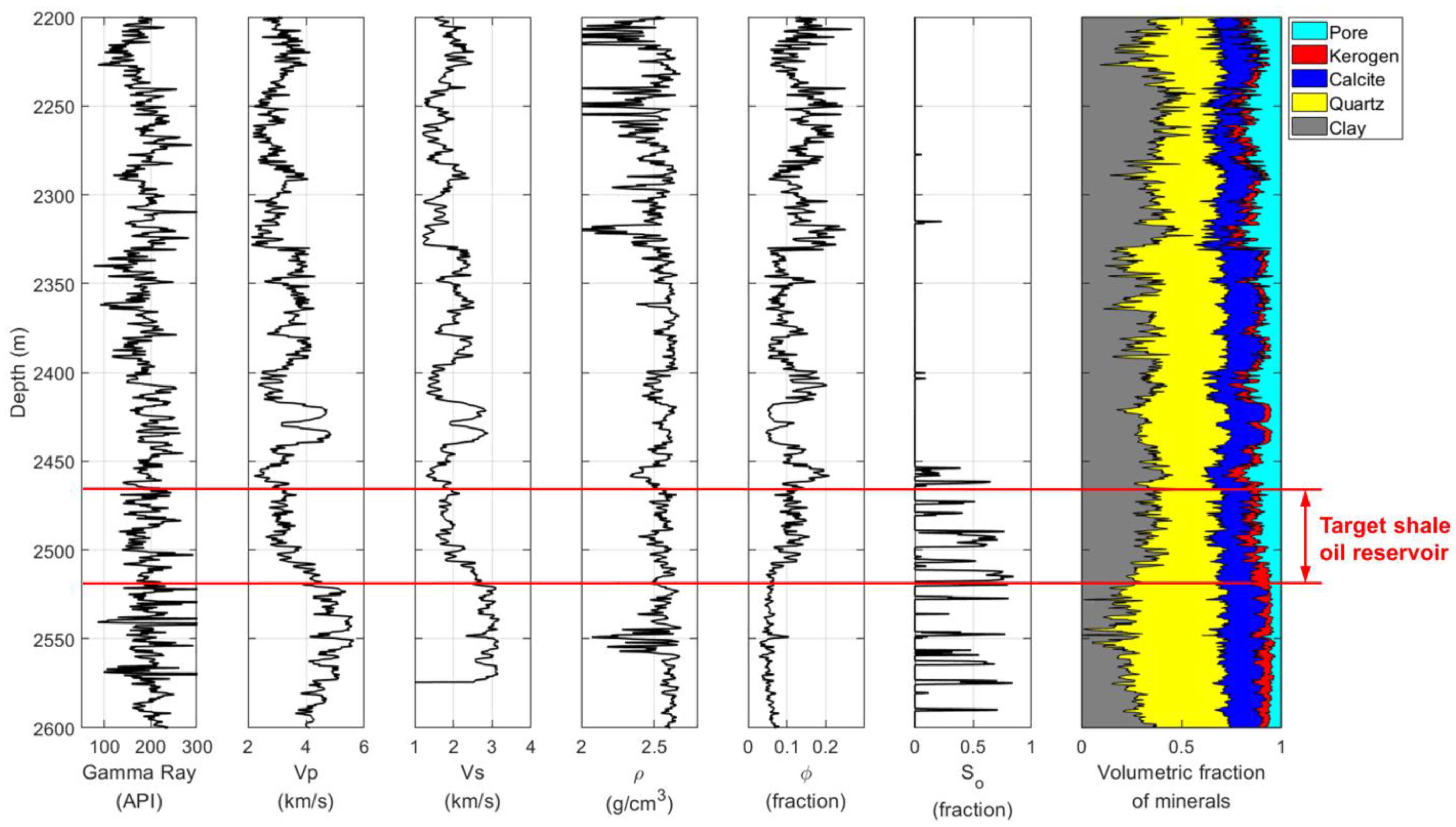
3.2. Prediction of the Horizontal Fracture Density by Using the Shale Model and Logging Data

Based on the shale model (see Figure 2) and the modeling framework (see Figure 3), the horizontal fracture porosity, ϕf, and the corresponding aspect ratio, α, have been calculated using logging data illustrated in Figure 8, with the obtained results presented in Figure 10. Table 1 presents the elastic properties of the components that were used in the modeling. The logarithmic value of the aspect ratio (log(α)) of the horizontal fracture was then used for simplicity In Figure 10, the modeled VP and VS according to Equations (14) and (15):
V P = c 33 ρ , V s = c 44 ρ
ρ = ( 1 φ ) i = 1 n f i ρ i + φ ρ f
where ρ represents the rock density, φ is the total porosity, and ρf is calculated using Equation (11). f1 and ρi are the volume fraction and density of each component, respectively. Elastic stiffnesses c33 and c44 are calculated using the Hudson model illustrated in Section 2.4.
As can be seen in Figure 10, the modeled VP and VS (red curves) were obtained using the fitting parameters ϕf and α. They clearly agree with the corresponding measured values (black curves), thereby validating the applicability of the modeling method. The predicted ϕf value shows how much pore space was occupied by horizontal fractures in the total porosity. In addition, the estimated α value shows the geometry of the horizontal fractures. According to Equation (7), it could be used to obtain the fracture density (εf), thereby providing a comprehensive evaluation of the horizontal fracture properties.

3.3. Obtaining the HF Indicator for the Horizontal Fracture Estimation of Shale Oil Reservoirs

Based on the results from the rock physical modeling (Figure 10), the HF indicator has been further evaluated according to Equation (13) for the evaluation of horizontal fractures in the shale oil reservoirs. As color-coded by εf in Figure 11, the cross-plots of IP and the VP/VS ratio have been obtained by using the results presented in Figure 10. The separable distributions of data clusters in the cross-plots showed the possibility for a determination of εf values from the elastic properties. Furthermore, the optimal rotation angle (θmax) in Equation (13) has been determined by using the framework of the Poisson impedance. As illustrated in Figure 12, a maximum correlation coefficient was found between εf and HF represented by elastic properties (IP and VP/VS) at θmax = 83°. Accordingly, the obtained HF indicator shows a good correlation with εf (Figure 13). Higher values of HF corresponded to an increase in εf, implying that the obtained HF acts as an effective indicator in the evaluation of the development of horizontal fractures in the shale. However, it must be stressed that since HF was obtained from the combination of IP and VP/VS, the values of HF in Figure 13 had no actual physical meaning.

3.4. Estimations of HF and TOC by Using Seismic Data

The obtained HF was further used for seismic data for a quantitative interpretation of the horizontal fractures. Figure 14 and Figure 15 illustrate the cross-well seismic profiles of IP and VP/VS, respectively. The HF factor, calculated from Figure 14 and Figure 15, was presented in Figure 16. To avoid any confusion, it should be noted that the HF factor in Figure 16 has been labeled using high and low magnitudes. The reason is that the HF value had no actual physical meaning, which has also been mentioned above in association with Figure 13.
As was discussed above, the obtained HF factor could be used as an effective indicator in the prediction of the development of horizontal fractures in shale oil reservoirs. The results presented in Figure 16 indicate that the target shale oil layer showed relatively large HF anomalies in the oil-producing wells A, B, and D, while exhibiting no anomalies in the dry well C. This consistency showed the importance of horizontal fractures for the ultimate productivity of shale oil reservoirs.
To further evaluate the importance of horizontal fractures for the ultimate oil productivity, the TOC of the shale oil reservoirs has been calculated based on the regression analysis of TOC versus density (ρ) by using logging data from well A (Figure 17). Subsequently, the TOC section (Figure 18) was derived from the seismic-inverted ρ based on the obtained linear regression presented in Figure 17. As can be seen in Figure 18, the target shale oil reservoir shows high TOC values for all oil wells (A, B, and D), and a relatively high TOC value for the dry well C. By comparing Figure 16 and Figure 18, the results indicate that the shale with the high TOC value, but a low horizontal fracture density (i.e., in well C), produces no oil. This shows that horizontal fractures are essential for the prediction of high-quality shale oil reservoirs.
Finally, the IP and VP/VS maps for the target shale oil reservoir are displayed in Figure 19 and Figure 20, respectively. Accordingly, the computed map of HF (Figure 21) is of great help for the comprehensive characterization of the shale oil reservoirs with simultaneous consideration of the TOC (Figure 22) derived from the seismic-inverted ρ.

4. Discussion

Numerous shale models have been proposed that relate the microstructures with the elastic properties of shale rocks. To achieve the objectives in the present study, appropriate modeling methods have been proposed to successfully predict horizontal fractures in the shales (Figure 1 and Figure 2). The main purpose of the proposed shale model was to quantify the elastic properties of the shale that has a total pore space occupied by matrix pores and horizontal fractures. In the modeling based on the shale model and logging data, horizontal fracture properties, ϕf and α, were estimated by using a rock physical inversion scheme (Figure 3). The obtained results were further used to derive the εf values for a comprehensive representation of the horizontal fractures (Figure 10). The modeling results showed that the modeled VP and VS fitted quite well with the measured VP and VS curves, which validated the applicability of the proposed shale model and the rationality of the calculated horizontal fracture properties (ϕf, α, and εf).
The separable distribution of data clusters in the cross-plot of IP and the VP/VS ratio showed that it is possible to determine εf using elastic properties (Figure 11). Accordingly, by using the framework of the Poisson impedance, the HF indicator was further proposed to estimate εf in terms of elastic properties (Equation (13)). With the calculated optimal rotation angle, the obtained HF factor showed a good correlation with εf. This result highlighted the effectiveness of HF in the evaluation of horizontal fractures in shale oil reservoirs (Figure 12 and Figure 13).
The obtained HF factor was further applied to seismic data for a quantitative interpretation of the horizontal fractures. The results showed that the shale oil reservoir had relatively high HF anomalies in the oil-producing wells A, B, and D, while exhibiting no anomalies in the dry well C (Figure 16). This regularity emphasized the importance of horizontal fractures for the ultimate productivity of the shale oil reservoirs.
The TOC section was further estimated by performing a regression analysis of TOC versus ρ. The effect of horizontal fractures on the ultimate oil productivity was thereby further evaluated. Also, a comparison of HF and TOC (Figure 16 and Figure 18, respectively) indicated that the shale with a high TOC value, but with a low horizontal fracture density, produced no oil. The results indicated that the horizontal fractures were important in the prediction of high-quality shale oil reservoirs. Nevertheless, other factors (including the TOC, brittleness of the reservoir, and hydraulic fracturing performance) should be considered for an effective evaluation of the shale oil reservoirs.

5. Conclusions

A framework that predicts horizontal fractures in shale oil reservoirs has been developed in the present study. A shale model was used as a rock physical modeling tool with logging data as input. An effective indicator for the evaluation of horizontal fractures was established by using the modeling results. The proposed indicator was then applied to seismic data for a quantitative interpretation of horizontal fractures in shale oil reservoirs by using seismic-inverted elastic properties. The main conclusions from this investigation were as follows:
(1)
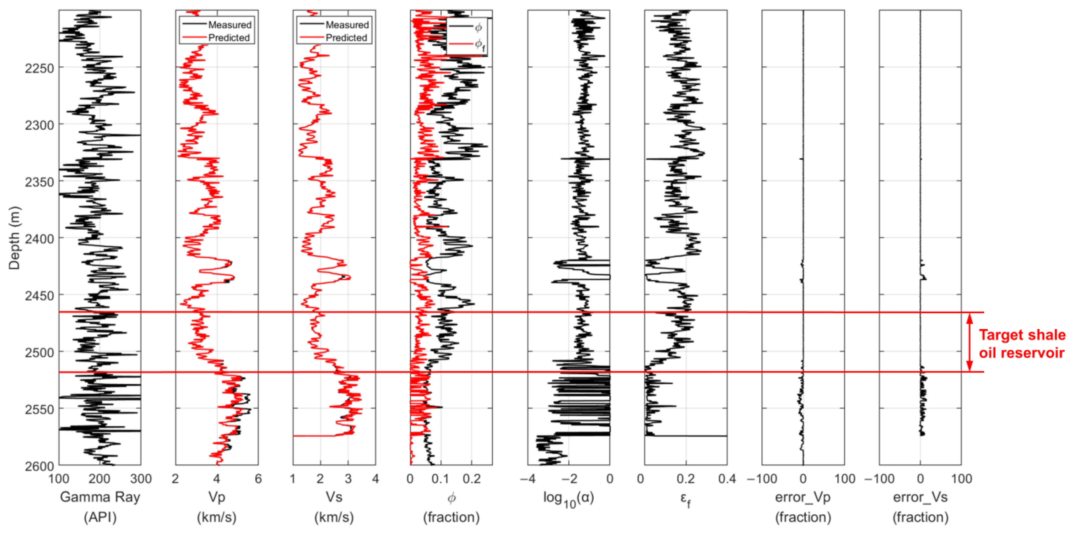
The proposed shale model was capable of quantifying the elastic responses of shale oil reservoirs that were associated with horizontal fracture properties. This result was validated by modeling results based on logging data. In the modeling, the calculated VP and VS showed a good agreement with the corresponding measured values. In addition, the predicted fracture properties, ϕf and α, were used to obtain the fracture density, εf, for further evaluation of horizontal fractures.
(2)
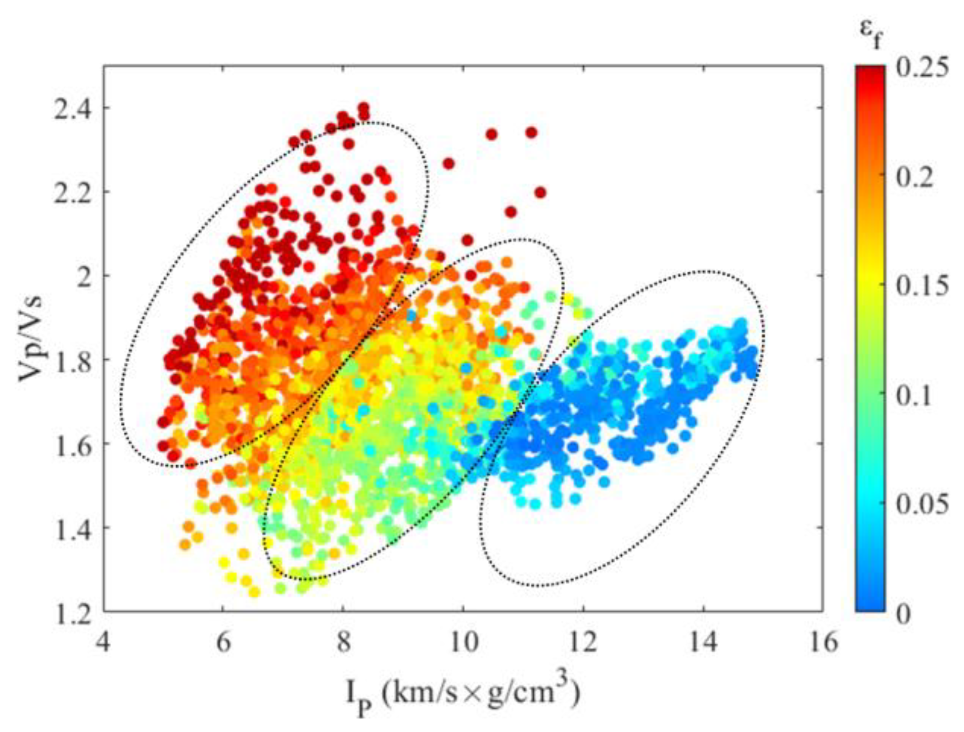
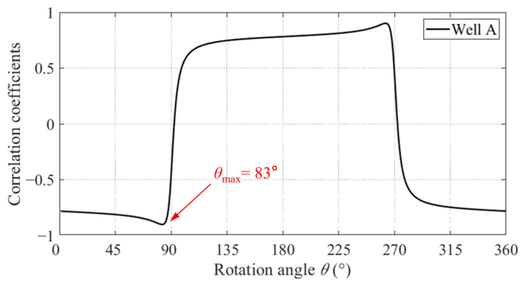
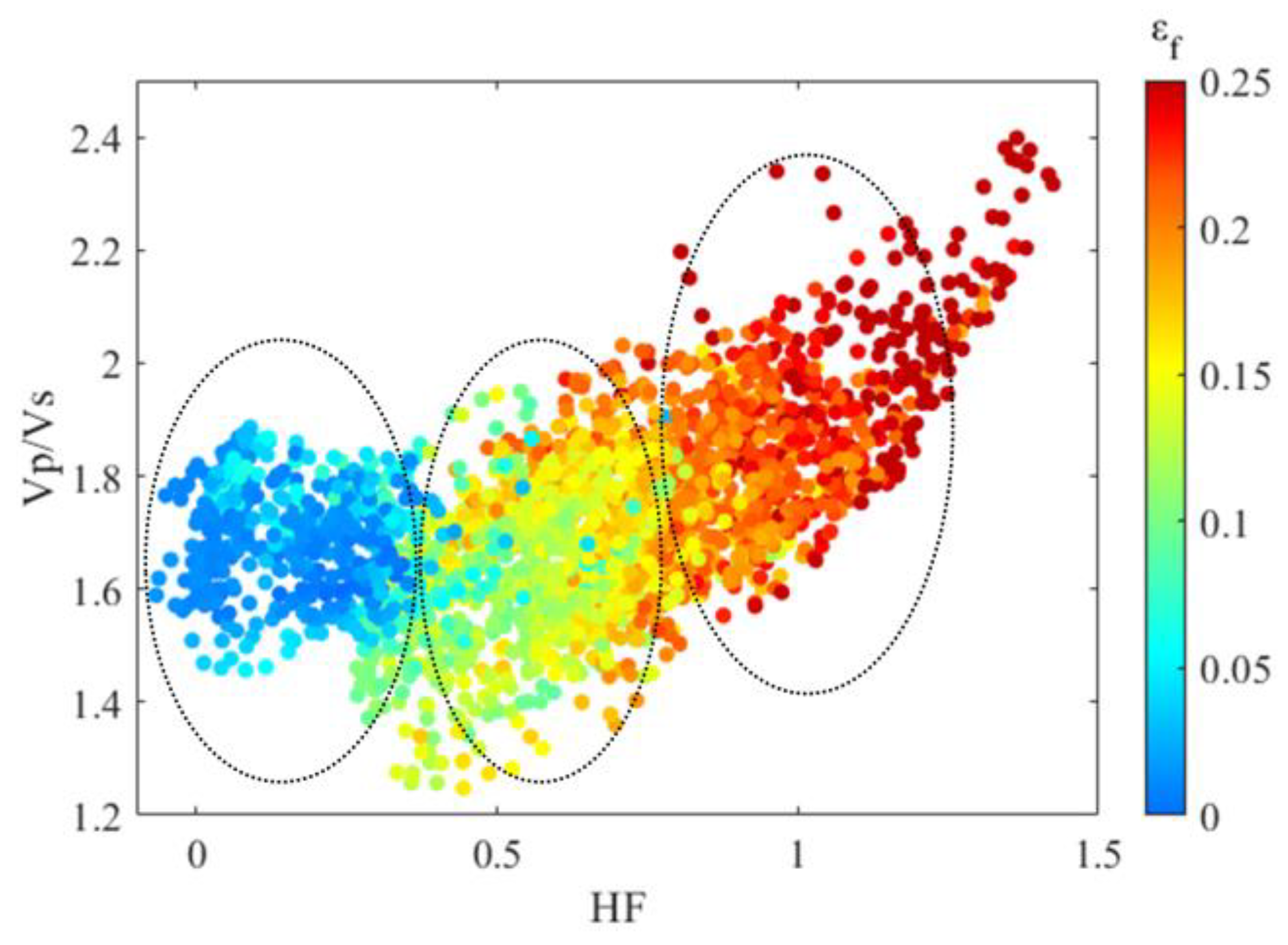
According to the framework of the Poisson impedance, the HF indicator was proposed to represent εf in terms of a combination of elastic properties (IP and VP/VS). This enabled a quantitative interpretation of the development of horizontal fractions by using seismic-inverted elastic properties. Also, the established HF indicator showed a good correlation with εf. The increasing HF indicated an increase in εf, which showed that the proposed HF factor was an effective indicator in the prediction of horizontal fractures in shale oil reservoirs.
(3)
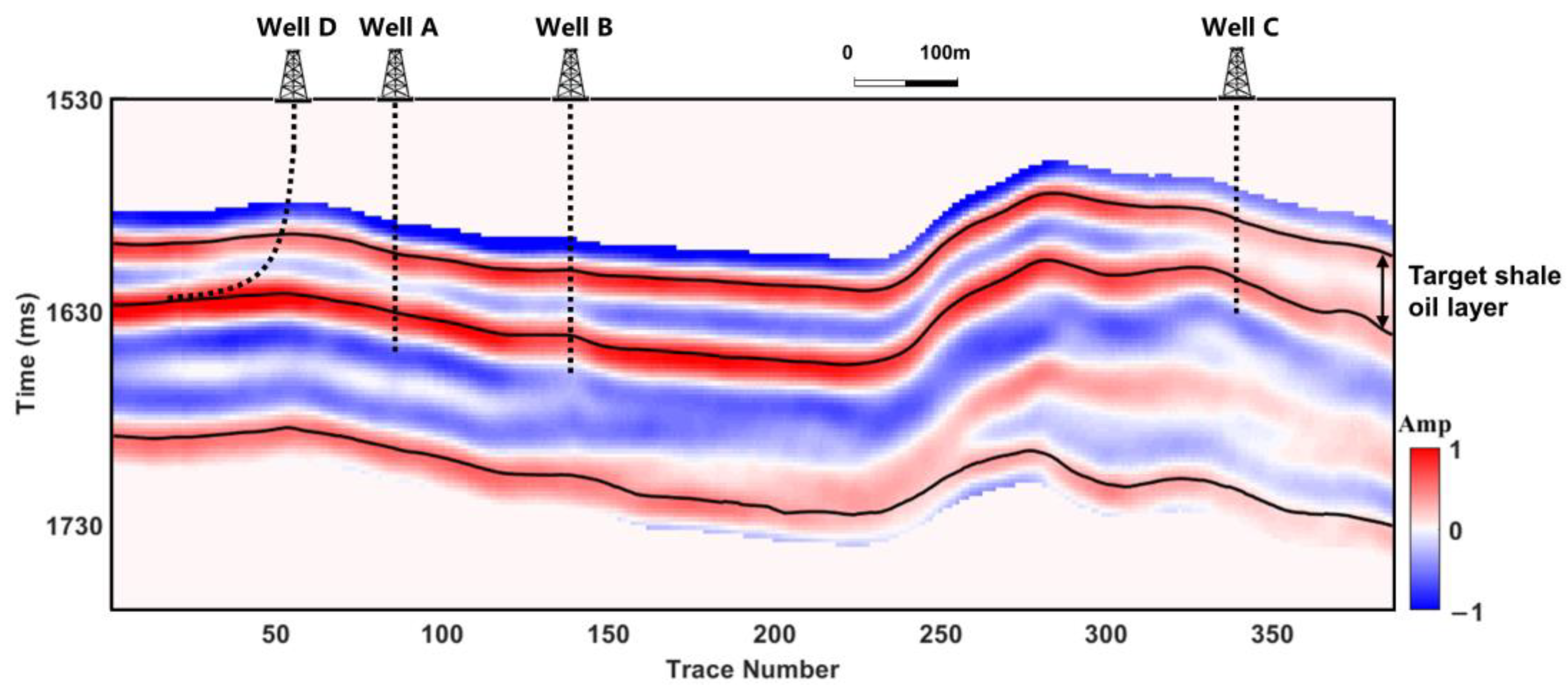
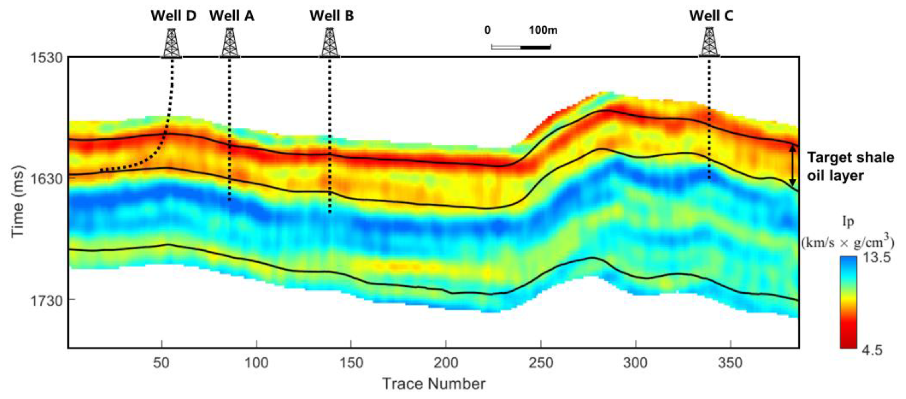
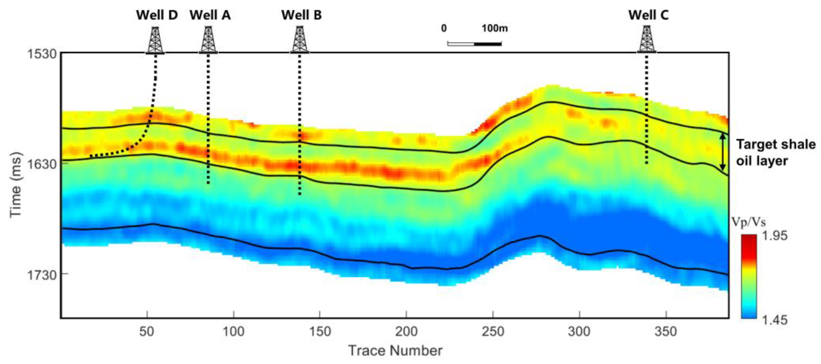
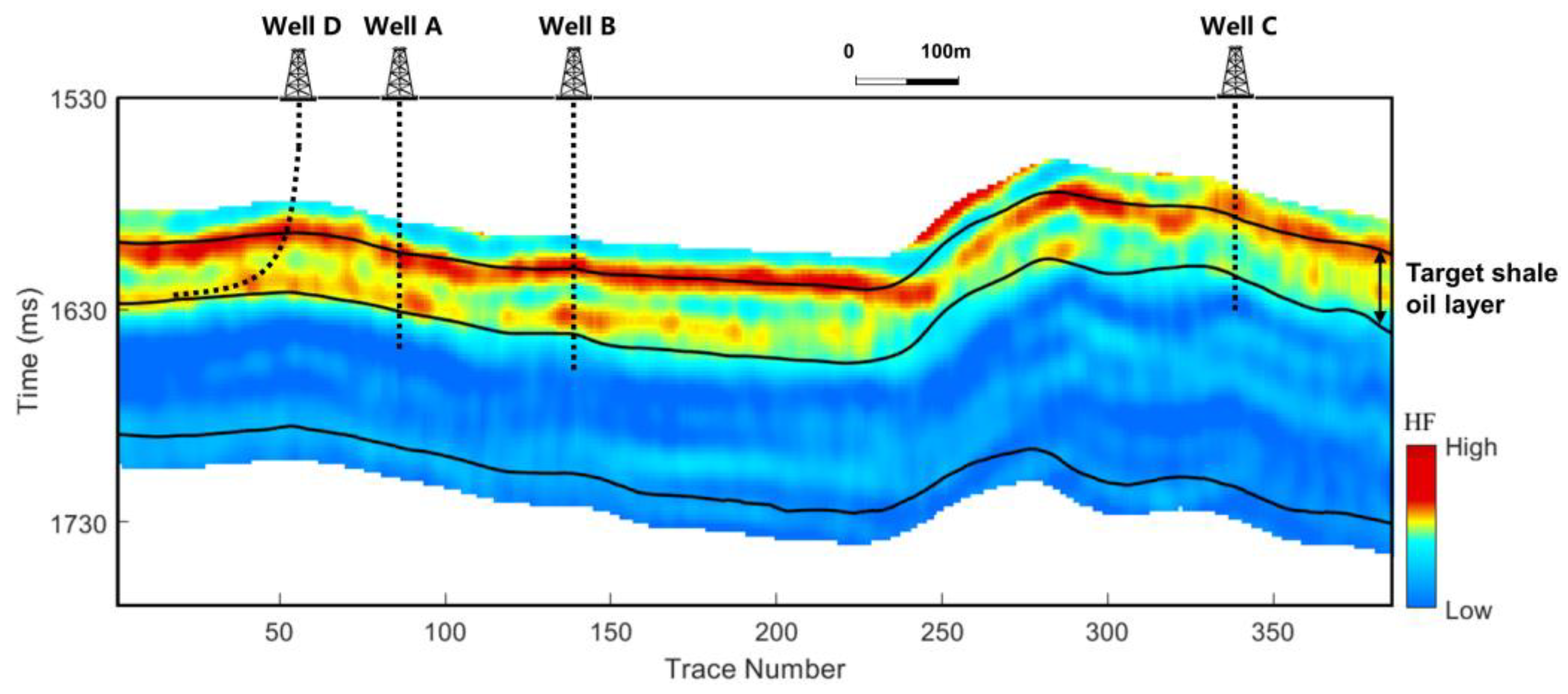
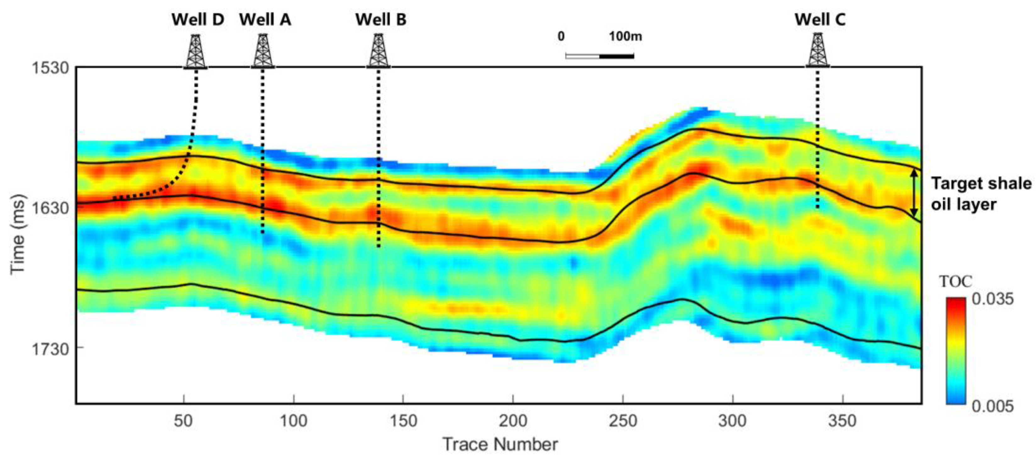
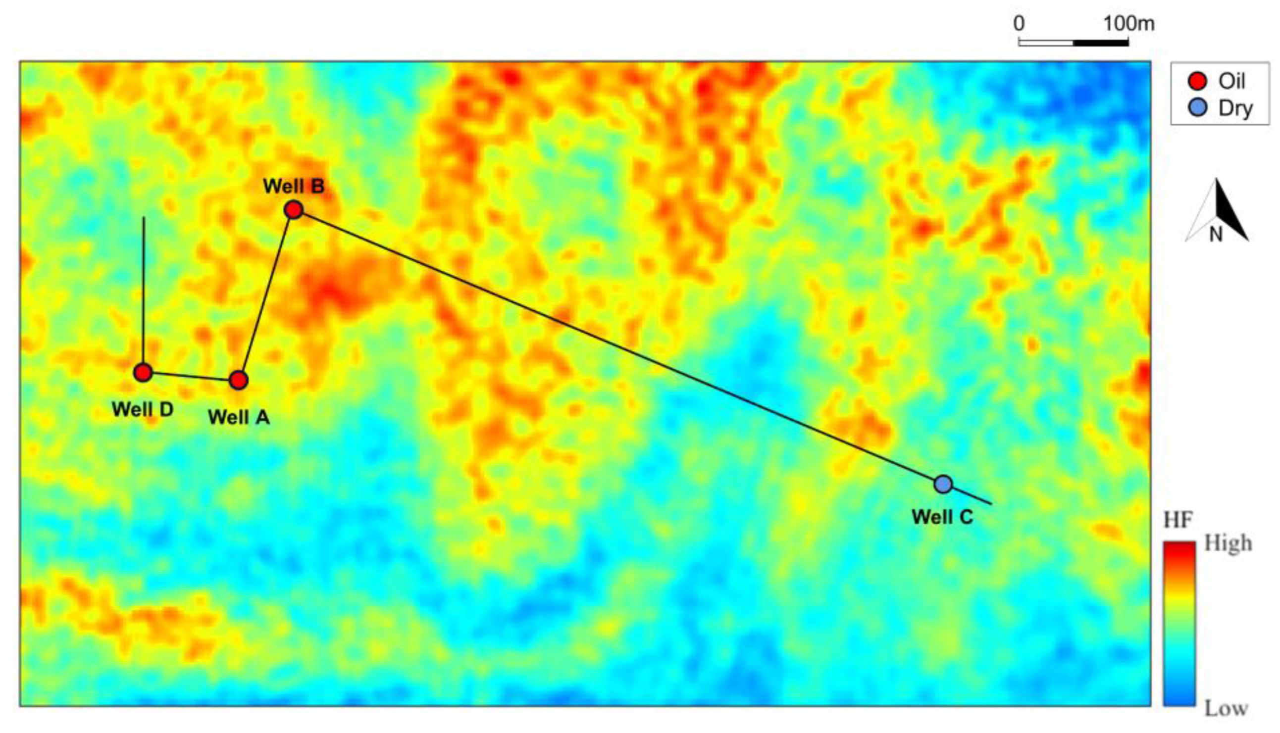
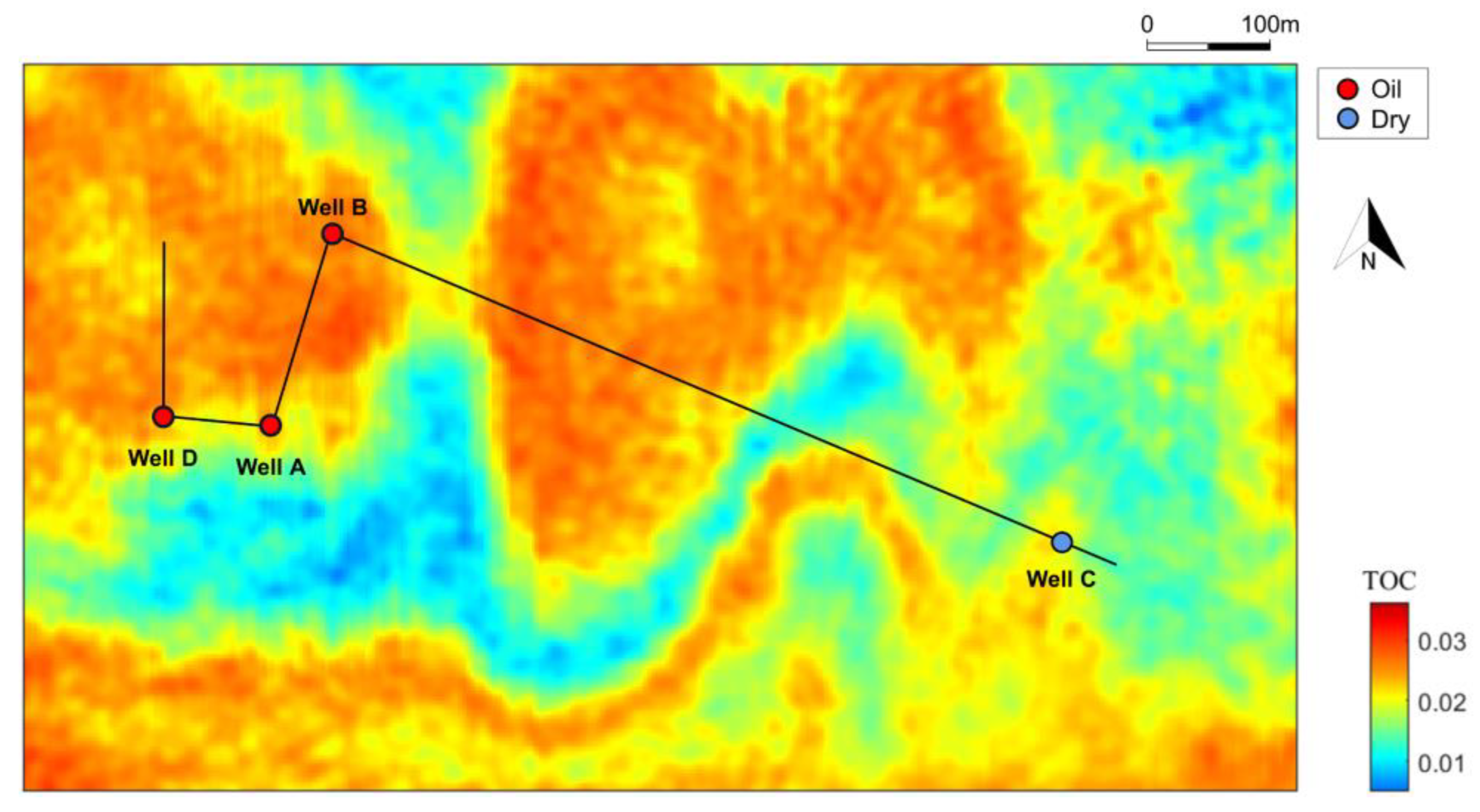
The seismic data applications showed that the target shale oil layer had high HF anomalies in the oil-producing wells, while exhibiting no anomalous response in the dry well. The consistency between the development of horizontal fractures and the production status of the boreholes highlighted the importance of horizontal fractures for the ultimate productivity of shale oil reservoirs. This result indicated that the horizontal fractures were essential in the prediction of high-quality shale oil reservoirs.
In future studies, the advancement of experiments and modeling methods can provide further insights into the effects of horizontal fractures on the seismic signatures of shale oil reservoirs. Based on these developments, other effective shale models, with corresponding parameters, can be developed for improved characterization of horizontal fractures in shale oil reservoirs.

Author Contributions

Conceptualization, Z.G.; methodology, Z.G.; software, W.G.; validation, Z.G. and W.G.; formal analysis, Z.G.; investigation, Z.G., W.G. and C.L.; resources, C.L.; data curation, W.G.; writing—original draft preparation, Z.G. and W.G.; writing—review and editing, Z.G.; visualization, W.G.; project administration, Z.G.; funding acquisition, Z.G. All authors have read and agreed to the published version of the manuscript.

Funding

This research was funded by the National Natural Science Foundation of China, grant numbers 42274160 and 42074153.

Data Availability Statement

Data are contained within the article.

Conflicts of Interest

The authors declare no conflict of interest.

References

  1. Xu, C.Y.; Zhu, L.M.; Xu, F.; Kang, Y.L.; Jing, H.R.; You, Z.J. Experimental study on the mechanical controlling factors of fracture plugging strength for lost circulation control in shale gas reservoir. Geoen. Sci. Eng. 2023, 231, 212285. [Google Scholar] [CrossRef]
  2. Diwu, P.X.; Liu, T.J.; You, Z.J.; Jiang, B.Y.; Zhou, J. Effect of low velocity non-Darcy flow on pressure response in shale and tight oil reservoirs. Fuel 2018, 216, 398–406. [Google Scholar] [CrossRef]
  3. Feng, G.J.; Zhu, Y.M.; Chen, S.B.; Wang, Y.; Ju, W.; Hu, Y.C.; You, Z.J.; Wang, G.G. Supercritical methane adsorption on shale over wide pressure and temperature ranges: Implications for gas-in-place estimation. Energy Fuel. 2020, 34, 3121–3134. [Google Scholar] [CrossRef]
  4. Xu, C.Y.; Kang, Y.L.; You, Z.J.; Chen, M.J. Review on formation damage mechanisms and processes in shale gas reservoir: Known and to be known. J. Nat. Gas Sci. Eng. 2016, 36, 1208–1219. [Google Scholar] [CrossRef]
  5. Vernik, L.; Milovac, J. Rock physics of organic shales. Lead. Edge 2011, 30, 318–323. [Google Scholar] [CrossRef]
  6. Zhao, L.X.; Qin, X.; Zhang, J.Q.; Liu, X.W.; Han, D.H.; Geng, J.H.; Xiong, Y.N. An Effective Reservoir Parameter for Seismic Characterization of Organic Shale Reservoir. Surv. Geophys. 2018, 39, 509–541. [Google Scholar] [CrossRef]
  7. Deng, X.H.; Liu, C.; Guo, Z.Q.; Liu, X.W.; Liu, Y.W. Rock physical inversion and quantitative seismic interpretation for the Longmaxi shale gas reservoir. J. Geophys. Eng. 2019, 16, 652–665. [Google Scholar] [CrossRef]
  8. Yin, L.J.; Yin, X.Y.; Zong, Z.Y.; Chen, B.C.; Chen, Z.Q. A new rock physics model method for shale on the theory of micro-nanopores. Chin. J. Geophys. 2020, 63, 1642–1653. [Google Scholar] [CrossRef]
  9. Guo, Z.Q.; Lv, X.Y.; Liu, C.; Liu, X.W.; Liu, Y.W. Shale gas characterisation for hydrocarbon accumulation and brittleness by integrating a rock-physics-based framework with effective reservoir parameters. J. Nat. Gas Sci. Eng. 2022, 100, 104498. [Google Scholar] [CrossRef]
  10. Goodway, B.; Varsek, J.; Abaco, C. Isotropic AVO methods to detect fracture prone zones in tight gas resource plays. In CSPG CSEG Convention; CSPG CSEG: Calgary, AB, Canada, 2007. [Google Scholar]
  11. Rickman, R.; Mullen, M.; Petre, E. A practical use of shale petrophysics for stimulation design optimization: All shale plays are not clones of the Barnett Shale. In Proceedings of the SPE Annual Technical Conference and Exhibition, Denver, CO, USA, 21–24 September 2008; SPE: Denver, CO, USA, 2008. [Google Scholar]
  12. Waters, G.A.; Lewis, R.E.; Bentley, D.C. The effect of mechanical properties anisotropy in the generation of hydraulic fractures in organic shales. In Proceedings of the SPE Middle East Unconventional Gas Conference and Exhibition, Denver, CO, USA, 30 October–2 November 2011; SPE: Abu Dhabi, United Arab Emirates, 2011. [Google Scholar]
  13. Slatt, R.M.; Abousleiman, Y. Merging sequence stratigraphy and geomechanics for unconventional gas shales. Lead. Edge 2011, 30, 274–282. [Google Scholar] [CrossRef]
  14. Guo, Z.Q.; Li, X.Y.; Liu, C.; Feng, X.; Shen, Y. A shale rock physics model for analysis of brittleness index, mineralogy and porosity in the Barnett Shale. J. Geophys. Eng. 2013, 10, 025006. [Google Scholar] [CrossRef]
  15. Chen, J.J.; Zhang, G.Z.; Chen, H.Z.; Yin, X.Y. The Construction of Shale Rock Physics Effective Model and Prediction of Rock Brittleness. In Proceedings of the SEG Annual Meeting, Denver, CO, USA, 26–31 October 2014; SEG: Denver, Colorado, USA, 2014. [Google Scholar]
  16. Bachrach, R.; Sengupta, M.; Salama, A.; Miller, P. Reconstruction of the layer anisotropic elastic parameters and high-resolution fracture characterization from P-wave data: A case study using seismic inversion and Bayesian rock physics parameter estimation. Geophys. Prospect. 2009, 57, 253–262. [Google Scholar] [CrossRef]
  17. Far, M.E.; Thomsen, L.; Sayers, C.M. Inversion for asymmetric fracture parameters using synthetic AVOA data. In Society of Exploration Geophysicists International Exposition; SEG: Las Vegas, NV, USA, 2012. [Google Scholar]
  18. Zhang, G.Z.; Chen, H.Z.; Yin, X.Y.; Li, N.; Yang, B.J. Method of Fracture Elastic Parameter Inversion Based on Anisotropic AVO. J. Jilin Univ. (Earth Sci. Ed.) 2012, 42, 845–851, 871. [Google Scholar] [CrossRef]
  19. Chen, H.Z.; Yin, X.Y.; Gao, C.G.; Zhang, G.Z.; Chen, J.J. AVAZ inversion for fluid factor based on fracture anisotropic rock physics theory. Chin. J. Geophys. 2014, 57, 968–978. [Google Scholar] [CrossRef]
  20. Chen, H.Z.; Zhang, G.Z.; Ji, Y.X.; Yin, X.Y. Azimuthal seismic amplitude difference inversion for fracture weakness. Pure Appl. Geophys. 2017, 174, 279–291. [Google Scholar] [CrossRef]
  21. Pan, X.; Zhang, G. Fracture detection and fluid identification based on anisotropic Gassmann equation and linear-slip model. Geophysics 2019, 84, R99–R112. [Google Scholar] [CrossRef]
  22. Luo, T.; Feng, X.; Guo, Z.; Liu, C.; Liu, X.W. Seismic AVAZ inversion for orthorhombic shale reservoirs in the Longmaxi area, Sichuan. Appl. Geophys. 2019, 16, 185–198. [Google Scholar] [CrossRef]
  23. Pan, X.P.; Zhang, P.F.; Zhang, G.Z.; Guo, Z.W.; Liu, J.X. Seismic characterization of fractured reservoirs with elastic impedance difference versus angle and azimuth: A low-frequency poroelasticity perspective. Geophysics 2021, 86, M123–M139. [Google Scholar] [CrossRef]
  24. Vernik, L.; Nur, A. Ultrasonic velocity and anisotropy of hydrocarbon source rocks. Geophysics 1992, 57, 727–735. [Google Scholar] [CrossRef]
  25. Vernik, L.; Landis, C. Elastic anisotropy of source rocks: Implications for hydrocarbon generation and primary migration. AAPG Bull. 1996, 80, 531–544. [Google Scholar] [CrossRef]
  26. Carcione, J.M. A model for seismic velocity and attenuation in petroleum source rocks. Geophysics 2000, 65, 1080–1092. [Google Scholar] [CrossRef]
  27. Carcione, J.M. AVO effects of a hydrocarbon source-rock layer. Geophysics 2001, 66, 419–427. [Google Scholar] [CrossRef]
  28. Carcione, J.M.; Helle, H.B.; Avseth, P. Source-rock seismic-velocity models: Gassmann versus Backus. Geophysics 2011, 76, N37–N45. [Google Scholar] [CrossRef]
  29. Sayers, C.M. The effect of kerogen on the AVO response of organic-rich shales. Lead. Edge 2013, 32, 1514–1519. [Google Scholar] [CrossRef]
  30. Sayers, C.M.; Guo, S.; Silva, J. Sensitivity of the elastic anisotropy and seismic reflection amplitude of the Eagle Ford Shale to the presence of kerogen. Geophys. Prospect. 2015, 63, 151–165. [Google Scholar] [CrossRef]
  31. Vernik, L. Hydrocarbon-generation-induced microcracking of source rocks. Geophysics 1994, 59, 555–563. [Google Scholar] [CrossRef]
  32. Vernik, L.; Liu, X. Velocity anisotropy in shales: A petrophysical study. Geophysics 1997, 62, 521–532. [Google Scholar] [CrossRef]
  33. Liu, J.; Ning, J.R.; Liu, X.W.; Liu, C.Y.; Chen, T.S. An improved scheme of frequency-dependent AVO inversion method and its application for tight gas reservoirs. Geofluids 2019, 2019, 3525818. [Google Scholar] [CrossRef]
  34. Zhang, X.M.; Shi, W.Z.; Hu, Q.H.; Zhai, G.Y.; Wang, R.; Xu, X.F.; Meng, F.L.; Liu, Y.Z.; Bai, L.H. Developmental characteristics and controlling factors of natural fractures in the lower paleozoic marine shales of the upper Yangtze Platform, southern China. J. Nat. Gas Sci. Eng. 2020, 76, 103191. [Google Scholar] [CrossRef]
  35. Xu, X.; Zeng, L.B.; Tian, H.; Ling, K.G.; Che, S.Q.; Yu, X.; Shu, Z.G.; Dong, S.Q. Controlling factors of lamellation fractures in marine shales: A case study of the Fuling Area in Eastern Sichuan Basin, China. J. Petrol. Sci. Eng. 2021, 207, 109091. [Google Scholar] [CrossRef]
  36. He, Z.L.; Li, S.J.; Nie, H.K.; Yuan, Y.S.; Wang, H. The shale gas “sweet window”: “The cracked and unbroken” state of shale and its depth range. Mar. Petrol. Geol. 2019, 101, 334–342. [Google Scholar] [CrossRef]
  37. Lu, Y.; Yang, F.; Bai, T.; Han, B.; Lu, Y.; Gao, H. Shale Oil Occurrence Mechanisms: A Comprehensive Review of the Occurrence State, Occurrence Space, and Movability of Shale Oil. Energies 2022, 15, 9485. [Google Scholar] [CrossRef]
  38. Gou, Q.; Xu, S. The Controls of Laminae on Lacustrine Shale Oil Content in China: A Review from Generation, Retention, and Storage. Energies 2023, 16, 1987. [Google Scholar] [CrossRef]
  39. Xu, S.; Gou, Q. The Importance of Laminae for China Lacustrine Shale Oil Enrichment: A Review. Energies 2023, 16, 1661. [Google Scholar] [CrossRef]
  40. Guo, Z.Q.; Liu, C.; Liu, X.W.; Dong, N.; Liu, Y.W. Research on anisotropy of shale oil reservoir based on rock physics model. Appl. Geophys. 2016, 13, 382–392. [Google Scholar] [CrossRef]
  41. Guo, Z.Q.; Zhang, X.D.; Liu, C.; Liu, X.W.; Liu, Y.W. Hydrocarbon identification and bedding fracture detection in shale gas reservoirs based on a novel seismic dispersion attribute inversion method. Surv. Geophys. 2022, 43, 1793–1816. [Google Scholar] [CrossRef]
  42. Zhao, L.X.; Qin, X.; Han, D.H.; Geng, J.H.; Yang, Z.F.; Cao, H. Rock-physics modeling for the elastic properties of organic shale at different maturity stages. Geophysics 2016, 81, 527–541. [Google Scholar] [CrossRef]
  43. Liu, X.W.; Guo, Z.Q.; Liu, C.; Liu, Y.W. Anisotropy rock physics model for the Longmaxi shale gas reservoir, Sichuan Basin, China. Appl. Geophys. 2017, 14, 21–30. [Google Scholar] [CrossRef]
  44. Guo, Z.Q.; Lv, X.Y.; Liu, C. Estimating Organic Enrichment in Shale Gas Reservoirs Using Elastic Impedance Inversion Based on an Organic Matter−Matrix Decoupling Method. Surv. Geophys. 2023, 44, 1985–2009. [Google Scholar] [CrossRef]
  45. Yi, S.; Pan, S.; Zuo, H.; Wu, Y.; Song, G.; Gou, Q. Research on Rock Physics Modeling Methods for Fractured Shale Reservoirs. Energies 2023, 16, 226. [Google Scholar] [CrossRef]
  46. Guo, Z.Q.; Li, X.Y.; Liu, C. Anisotropy parameters estimate and rock physics analysis for the Barnett Shale. J. Geophhys. Eng. 2014, 11, 065006. [Google Scholar] [CrossRef]
  47. Sayers, C.M.; den Boer, L.D. The elastic properties of clay in shales. J. Geophys. Res. Sol. Ea. 2018, 123, 5965–5974. [Google Scholar] [CrossRef]
  48. Li, X.; Chen, K.; Li, P.; Li, J.; Geng, H.; Li, B.; Li, X.; Wang, H.; Zang, L.; Wei, Y.; et al. A New Evaluation Method of Shale Oil Sweet Spots in Chinese Lacustrine Basin and Its Application. Energies 2021, 14, 5519. [Google Scholar] [CrossRef]
  49. Hashin, Z.; Shtrikman, S. A variational approach to the theory of the elastic behaviour of multiphase materials. J. Mech. Phys. Solids 1963, 11, 127–140. [Google Scholar] [CrossRef]
  50. Berryman, J.G. Long-wavelength propagation in composite elastic media II. Ellipsoidal inclusions. J. Acoust. Soc. Am. 1980, 68, 1820–1831. [Google Scholar] [CrossRef]
  51. Hudson, J.A. Overall properties of a cracked solid. Math. Proc. Camb. Phil. Soc. 1980, 88, 371–384. [Google Scholar] [CrossRef]
  52. Domenico, S.N. Elastic properties of unconsolidated porous sand reservoirs. Geophysics 1977, 42, 1339–1368. [Google Scholar] [CrossRef]
  53. Quakenbush, M.; Shang, B.; Tuttle, C. Poisson impedance. Lead. Edge 2006, 25, 128–138. [Google Scholar] [CrossRef]
  54. Tian, L.X.; Zhou, D.H.; Lin, G.K.; Jiang, L.C. Reservoir prediction using Poisson impedance in Qinhuangdao, Bohai Sea. In SEG Annual Meeting; European Association of Geoscientists & Engineers: Denver, CO, USA, 2010. [Google Scholar]
  55. Ming, J.; Qin, D.H. An effeictive method of fluid discrimination using Poisson impedance and multi-attribute inversion. In SEG International Exposition and Annual Meeting; Society of Exploration Geophysicists: Dallas, TX, USA, 2016. [Google Scholar]
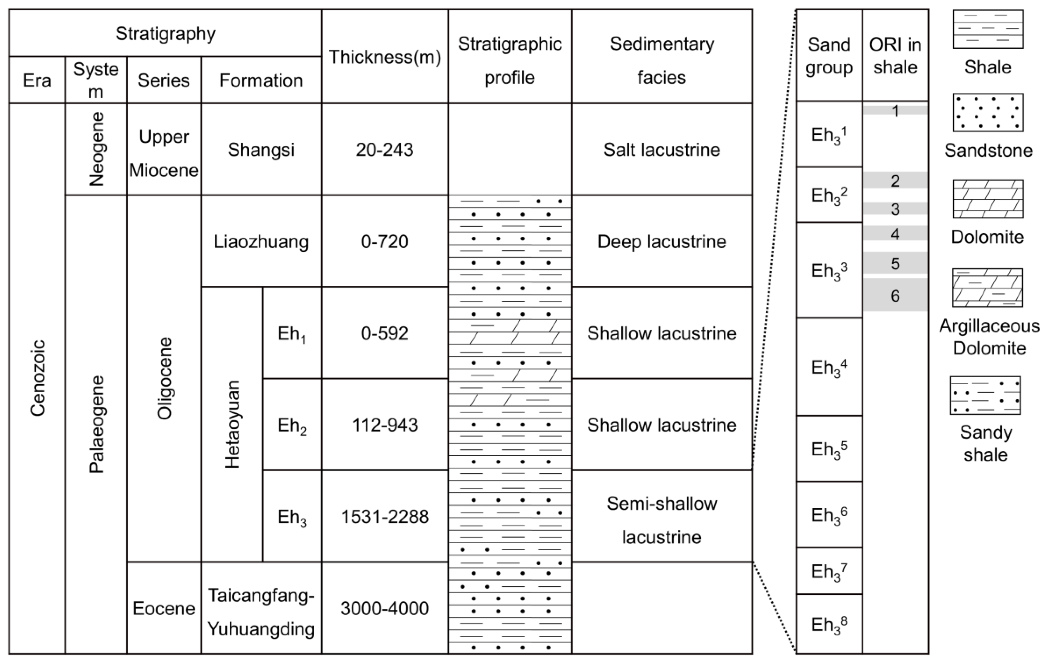
  56. Shang, F.; Xie, X.N.; Li, S.F. Enrichment conditions of Hetaoyuan Formation shale oil in Biyang Depression, China. J. Pet. Explor. Prod. Technol. 2019, 9, 927–936. [Google Scholar] [CrossRef]
  57. Li, L.J.; Lyu, Q.Q.; Shang, F. Seismic prediction of lithofacies heterogeneity in paleogene hetaoyuan shale play, Biyang depression, China. Open Geosci. 2020, 12, 1383–1391. [Google Scholar] [CrossRef]
  58. Mavko, G.; Mukerji, T.; Dvorkin, J. The Rock Physics Handbook: Tools for Seismic Analysis in Porous Media; Cambridge University Press: Cambridge, UK, 2009. [Google Scholar]
Figure 1. Flowchart of rock physical modeling for shale oil reservoirs.
Energies 16 07514 g001
Figure 2. Schematics of the pore spaces in the shale matrix, which consist of matrix pores and horizontal fractures.
Energies 16 07514 g002
Figure 3. Workflow for the prediction of horizontal fractures using the shale model and well-log data.
Energies 16 07514 g003
Figure 4. (a) Location of the Nanxiang Basin in China, (b) Location of the Biyang Sag in the Nanxiang Basin, where the red rectangle indicates the studied area in the present investigation.
Energies 16 07514 g004
Figure 5. Stratigraphic units and sedimentary facies in the studied area.
Energies 16 07514 g005
Figure 6. Two-way time (TWT) for the shale oil reservoir. The red and blue dots indicate the locations of oil and dry wells, respectively. The straight lines denote the seismic lines across the wells.
Energies 16 07514 g006
Figure 7. Seismic profile across the wells.
Energies 16 07514 g007
Figure 8. Logging curves from well A, including the gamma-ray (GR) values, P-wave velocity (VP), S-wave velocity (VS), density (ρ), porosity (ϕ), oil saturation (So), and volumetric fraction of minerals.
Energies 16 07514 g008
Figure 9. Formation micro-scanner image (FMI) for the target shale layer in well A.
Energies 16 07514 g009
Figure 10. Logging curves and rock physical modeling results for well A, including curves of the gamma-ray (GR) value, P-wave velocity (VP), S-wave velocity (VS), porosity (ϕ), logarithm value of the horizontal fracture aspect ratio (log(α)), fracture density (εf), relative error of VP (error_VP), and relative error of VS (error_VS).
Energies 16 07514 g010
Figure 11. Cross-plot of IP and VP/VS, as color-coded by εf.
Energies 16 07514 g011
Figure 12. Correlation coefficient variations with the rotation angle, θ.
Energies 16 07514 g012
Figure 13. Cross-plot of HF (θmax = 83°) and VP/VS, as color-coded by εf.
Energies 16 07514 g013
Figure 14. Profile of the IP crossing wells.
Energies 16 07514 g014
Figure 15. Profile of the VP/VS crossing wells.
Energies 16 07514 g015
Figure 16. Profile of the HF crossing wells.
Energies 16 07514 g016
Figure 17. Linear regression of TOC versus ρ, using logging data from well A.
Energies 16 07514 g017
Figure 18. Profile of the TOC crossing wells.
Energies 16 07514 g018
Figure 19. Horizontal map of IP for the target shale.
Energies 16 07514 g019
Figure 20. Horizontal map of VP/VS for the target shale.
Energies 16 07514 g020
Figure 21. Horizontal map of HF for the target shale.
Energies 16 07514 g021
Figure 22. Horizontal map of TOC for the target shale.
Energies 16 07514 g022
Table 1. Properties of the components that have been used for the modeling [58].
ClayQuartzCalciteKerogenOilWater
VP (km/s)3.66.056.842.60.91.47
VS (km/s)1.854.36 3.721.500
ρ (g/cm3)2.582.652.751.350.71.04
Disclaimer/Publisher’s Note: The statements, opinions and data contained in all publications are solely those of the individual author(s) and contributor(s) and not of MDPI and/or the editor(s). MDPI and/or the editor(s) disclaim responsibility for any injury to people or property resulting from any ideas, methods, instructions or products referred to in the content.

