Semi-Analytical Reservoir Modeling of Non-Linear Gas Diffusion with Gas Desorption Applied to the Horn River Basin Shale Gas Play, British Columbia (Canada)

Abstract

Adsorbed gas may account for a significant part of the gas resources in shale gas and coalbed methane plays. Understanding gas sorption behaviors and integrating gas desorption into analytical reservoir modeling and an associated transient performance analysis are important for evaluating a system’s gas desorption ability and further analyzing its CO₂ injectability, utilization, and storage capacity. However, gas desorption, along with other pressure-dominated gas properties, increases a system’s non-linearity in theoretical studies. Few studies on analytical modeling have integrated the gas desorption feature into a non-linear system and validated the model’s accuracy. In this study, the desorbed gas due to pressure decay was treated as an additional source/sink term in the source-and-sink function methods. This method was combined with the integral image method in a semi-analytical manner to determine the amount of gas desorption. Fundamental reservoir and gas properties from the Horn River Basin shale gas play were chosen to evaluate the methodology and the performance of the associated production well. The results were compared with the commercial fine-gridding numerical simulation software, and good matches were achieved. The results showed that the desorbed gas released from rock will supply free-gas flow when the pressure significantly decreases due to gas production. The production wellbore pressure can be maintained at a higher level, and the production rate was higher than in cases where gas desorption was not considered, depending on the operating conditions.

1. Introduction

Organic-rich shale and coalbed methane (CBM), which serve as sources of low-carbon fossil fuels, will play an important role in the future development of a clean energy supply; CO₂ capture, utilization, and storage (CCUS); and geothermal energy production. Natural gas is seen as a relatively cleaner-burning fossil fuel than coal and petroleum products, as it generates fewer emissions of air pollutants and CO₂ [1] while still providing a high calorific value [2]. The development of unconventional gas resources has significantly changed the global gas supply market, and the U.S. has become a self-sufficient-energy country after the evolution of hydraulic fracturing technology, as an example [3,4]. CCUS is one of the most promising methods for reaching a net-zero-emissions goal, and depleted shale gas and CBM could be good potential formations for geological carbon storage [5,6,7,8,9]. Molecular models have shown that the adsorption of CO₂ can promote CH₄ desorption [10], which enhances the gas production in shale and CBM and the storage of more CO₂ through geological sequestration. Many shale gas and CBM formations are also sources of geothermal energy [11,12] and thermal energy storage [13]. As a result, unconventional gas resources such as shale and CBM are critical to the future energy industry, and studies on their resource characterization, storage mechanisms, and flow regimes are important to understanding their resource production and their potential for applications in CCUS and geothermal energy production.

Gas adsorption is one of the primary storage mechanisms of natural gas resources in shale gas and CBM [14]. Compared to conventional gas reservoirs, shale gas and CBM present greater difficulties in estimating their gas production because of their gas desorption mechanism [15,16]. In shales, gas is physically adsorbed (Figure 1) on organic matter because the attractive intermolecular forces between the solid surface and natural gas are greater than those between gas molecules [17,18]. The Langmuir isotherm is widely used to describe the gas desorption in shale gas reservoirs [15,18,19,20]. The maximum adsorbed gas volume can be affected by clay minerals, the pressure, the temperature, the water/moisture content, the thermal maturity, and the kerogen types [18,21,22,23,24]. However, many publications and laboratory data suggest that the organic richness, or the total organic carbon (TOC), primarily controls the adsorption feature in shale gas reservoirs [18,22,25,26,27]. During the shale gas production process, the free gas existing in the porous rock matrix (organic and inorganic) and fractures will first be driven towards producers by the pressure gradient. The adsorbed gas will then be released from the solid surface due to the pressure depletion and become the new free-gas phase. Among the gas in reservoirs, adsorbed shale gas accounts for 20–80% [19,20] of the total original gas in place (OGIP). Considering future CO₂ sequestration and geothermal energy production, accurately evaluating the shale gas adsorption/desorption behavior through the transient performance of the production wellbore is essential.

Analyzing the transient performance of unconventional gas reservoirs using equations has historically been a challenge due to their high non-linear gas diffusion and adsorption/desorption behavior. In general, pseudo-functions are applied to integrate the pressure-dependent variables into pressure and time terms [28,29,30,31]. As a result, the non-linearity of the system due to its pressure-dependent gas properties can be linearized, and the equation can be solved analytically. Recent works have mainly focused on modeling the performance of hydraulic fracturing wells in tight and shale reservoirs [32,33,34,35]. Few studies have integrated shale gas desorption into reservoir-scale modeling [36], and fundamental research on the effect of gas desorption needs to be conducted and validated. This work presents an analytical approach using an additional source/sink method to describe non-linear gas diffusion processes and reveal the transient behavior of the pressure decline in a shale gas reservoir with the gas desorption mechanism. The proposed analytical method uses linearized gas diffusivity equations, based on pseudo-pressure and pseudo-time, and the integral image method (IIM) for reservoir-scale modeling. The pseudo-time was converted back to the real-time domain by resolving the reservoir’s average pressure in the region of investigation using an iterative procedure in the Laplace domain. Gas desorption was analytically treated as an additional source/sink with a variable rate within each discretized reservoir domain. The proposed method was then applied to the Horn River shale gas play to examine the gas desorption and flow behaviors in relation to the production performance.

2. Methodology

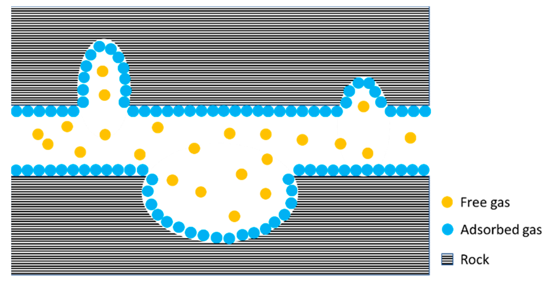
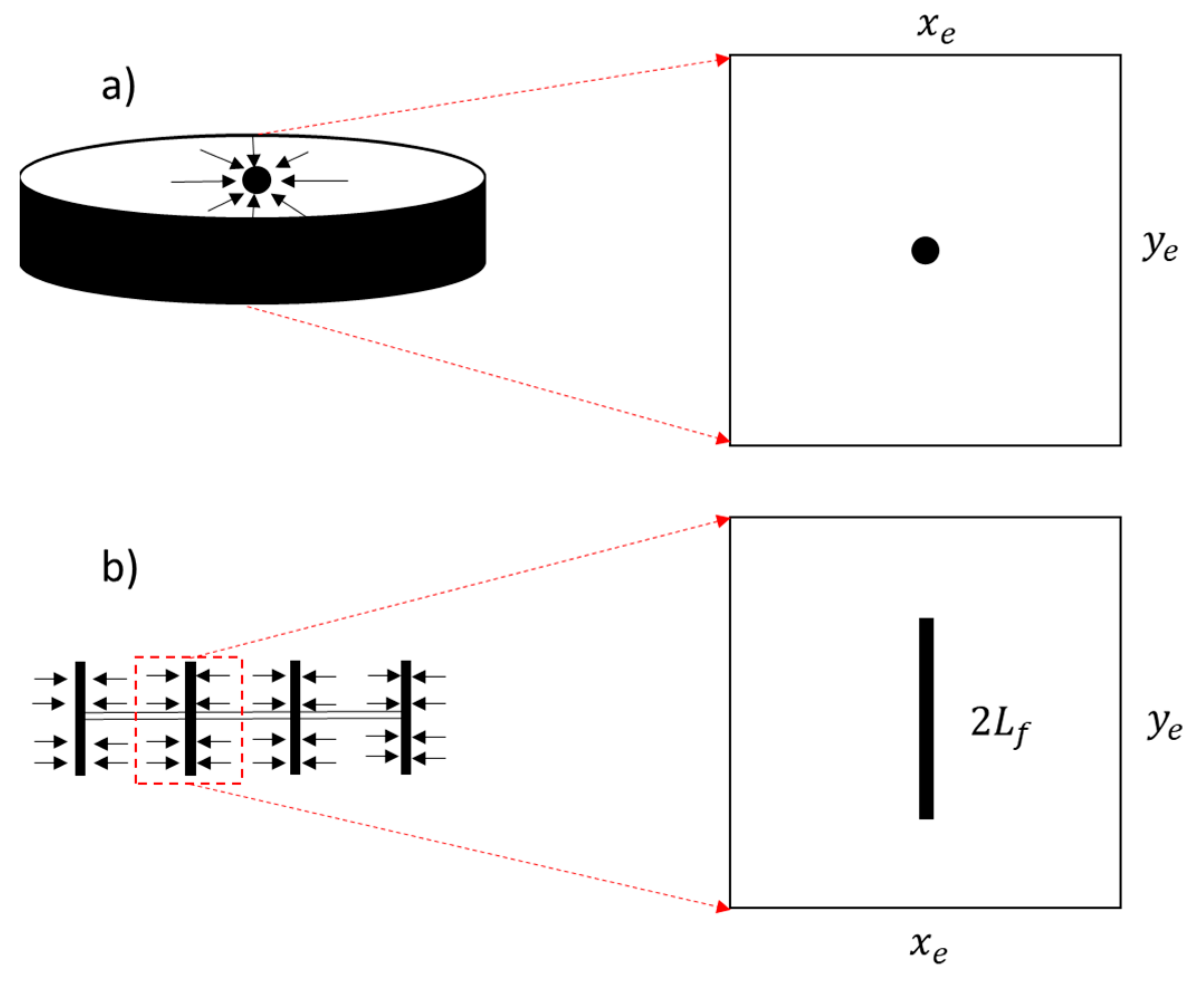
2.1. Gas Diffusion Process

The natural gas diffusion process in porous media can be characterized by a combination of the mass conservation principle and the gas-phase equation of state (EOS). The continuity equation of gas diffusion is expressed as:

$$\nabla \left(\frac{p}{{\mu }_g{z}_g}k\nabla p\right)=\varphi \frac{\partial }{\partial t}\left(\frac{p}{z_g}\right)$$

(1)

where p is the pressure of the gas phase, k is the gas-phase permeability, $\varphi$ is the rock porosity, ${\mu }_g$ is the viscosity of natural gas, $z_g$ is the gas compressibility factor, and t is the time. In this equation, the viscosity and gas compressibility factor are dependent on the pressure, making the diffusion equation non-linear. Pseudo-pressure (Equation (2)) and pseudo-time (Equation (3)) were applied to integrate the pressure-dependent variables in the continuity equation (Equation (1)) and linearize the system:

$$m\left(p\right)={\int }_{p^{\ast }}^p\frac{p}{{\mu }_g{z}_g}dp$$

(2)

$$t_a={\int }_0^t\frac{k}{\varnothing c_g\left(\tau \right){\mu }_g\left(\tau \right)}d\tau$$

(3)

where $p^{\ast }$ is the reference pressure; $c_g$ is the gas compressibility, which can be expressed by a function of p and z_g; and $\tau$ is the time integral variable. The linearized gas diffusion equation is then expressed as follows:

$${\nabla }^{2}m=\frac{\partial m}{\partial t_a}$$

(4)

By applying the source-and-sink function methods first used in the mathematical description of variable temperature cases of heat conduction in solids [37] and Newman’s product [38], the point-source/sink solution of the pseudo-pressure change in a 2D system can be expressed as follows:

$$∆m\left(x,x^{\prime },y,y^{\prime },t_a\right)=\frac{p_{std}}{kh}·\frac{T_{res}}{T_{std}}{\int }_o^{t_a}{q}_{std}\left({\tau }_a\right)\frac{1}{4\pi \left(t_a-{\tau }_a\right)}exp\left[-\frac{{\left(x-x^{\prime }\right)}^2+{\left(y-y^{\prime }\right)}^2}{4\left(t_a-{\tau }_a\right)}\right]d{\tau }_a$$

(5)

where $p_{std}$ and $T_{std}$ are the pressure and temperature under standard conditions, respectively; $T_{res}$ is the temperature under reservoir conditions; h is the reservoir thickness in this 2D system; $q_{std}$ is the gas source/sink flow rate under standard conditions; x and y are the coordinates of any point; $x^{\prime }$ and $y^{\prime }$ are the coordinates of the source/sink point; and ${\tau }_a$ is the instantaneous pseudo-time. Further details on the use of source-and-sink functions to solve problems regarding the fluid flow and heat transfer in porous media are given in previous studies [39,40,41,42].

Dimensionless terms could help generate a universal solution and the results could be applied for further type-curve matching. The related dimensionless terms are defined as follows:

$$m_D=\frac{2\pi kh}{q_{std\_unit}·\frac{T_{res}·p_{std}}{T_{std}}}·∆m$$

(6)

$$t_D=\frac{t_a}{l_{reference}^2}$$

(7)

$$q_D=\frac{q_{std}}{q_{std\_unit}}$$

(8)

$$x_D=\frac{x}{l_{reference}}$$

(9)

$$y_D=\frac{y}{l_{reference}}$$

(10)

$${x^{\prime }}_D=\frac{x^{\prime }}{l_{reference}}$$

(11)

$${y^{\prime }}_D=\frac{y^{\prime }}{l_{reference}}$$

(12)

where $q_{std\_unit}$ is the unit flow rate of the gas source/sink under standard conditions and $l_{reference}$ is the reference length. The dimensionless solution of the gas reservoir point source can be rewritten as follows:

$$m_D\left(x_D,x_D^{\prime },y_D,y_D^{\prime },t_D\right)={\int }_0^{t_D}{q}_D\left({\tau }_D\right)·\frac{1}{2\left(t_D-{\tau }_D\right)}exp\left[-\frac{{\left(x_D-{x^{\prime }}_D\right)}^2+{\left(y_D-{y^{\prime }}_D\right)}^2}{4\left(t_D-{\tau }_D\right)}\right]d{\tau }_D$$

(13)

In order to inverse the dimensionless results to dimensional space, the pseudo-pressure and pseudo-time need to be evaluated back to the pressure and time domains. A curve of the pseudo-pressure vs. pressure was generated using the gas-phase properties, either from lab tests or empirical formulas. The pressure was then calculated through interpolation from the data set. In terms of evaluating the pseudo-time, the use of the average pressure in the drainage area was proposed to determine the numerical integral. The time was expressed using the inverse of the pseudo-time:

$$t={\int }_0^{t_a}\frac{\varnothing c_g\left({\tau }_a\right){\mu }_g\left({\tau }_a\right)}{k}d{\tau }_a$$

(14)

For the pressure-dependent variables $c_g$ and ${\mu }_g$, the average pressure in the drainage area was used to calculate their values at each time point. The drainage area was defined as the area where the pressure changed compared to the initial reservoir pressure. In dimensionless terms, it was the area where $m_D$ was not equal to zero (Figure 2).

The average pressure can be calculated using the volumetric average:

$$p_{ave}\left(t\right)=\frac{\int p\left(t\right)d{V}_d}{\int d{V}_d}$$

(15)

where $V_d$ is the volume of the reservoir in the drainage area. A verification case study of a point source in the center of a square-shaped 2D reservoir was conducted to examine the pseudo-pressure and pseudo-time system. The pressure decline under a constant production rate is plotted in Figure 3. The result was compared with a commercial software, the KAPPA Workstation Saphir V.5.50 module. A highly accurate result was achieved by using the pseudo-pressure and pseudo-time methodology in the gas diffusion process.

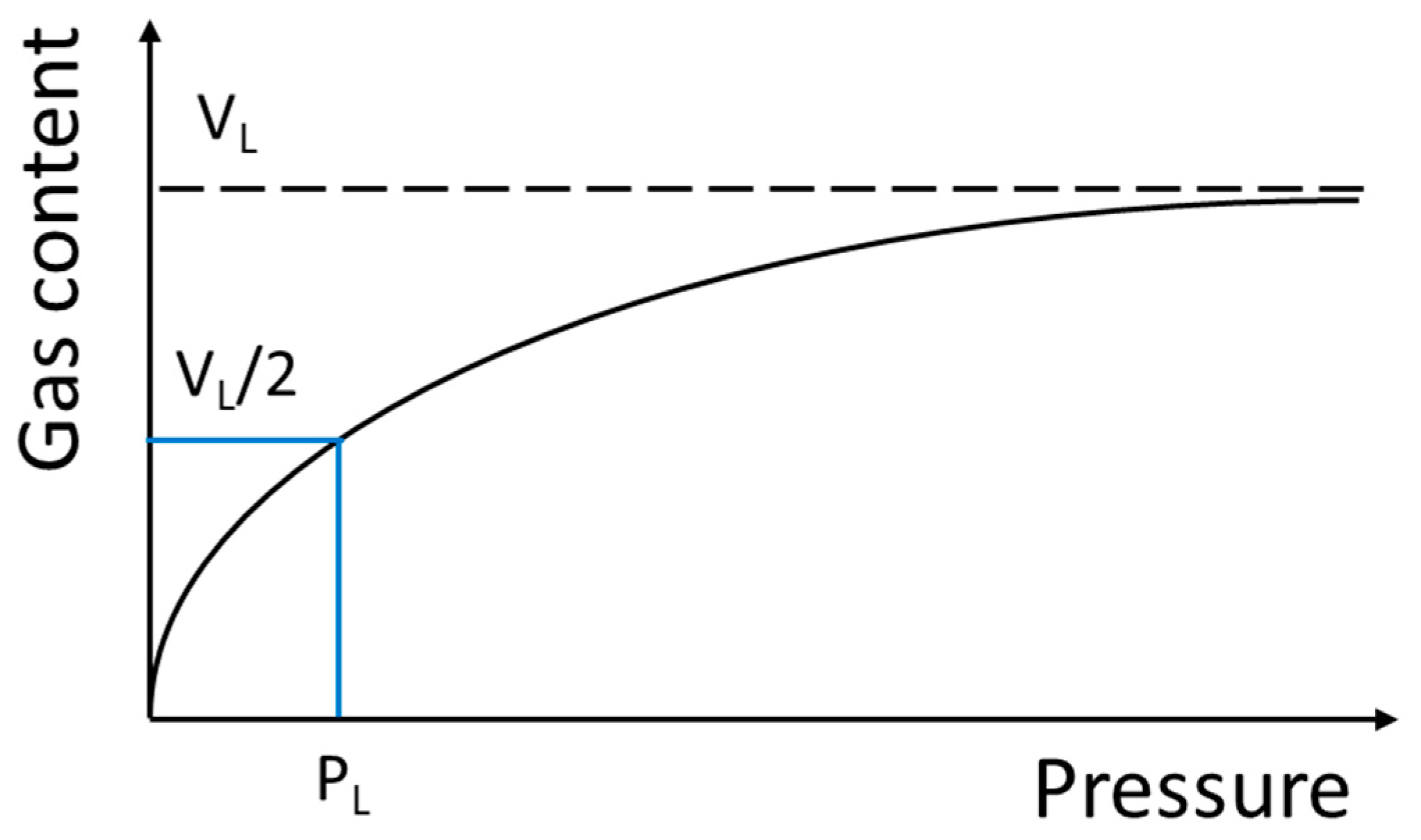
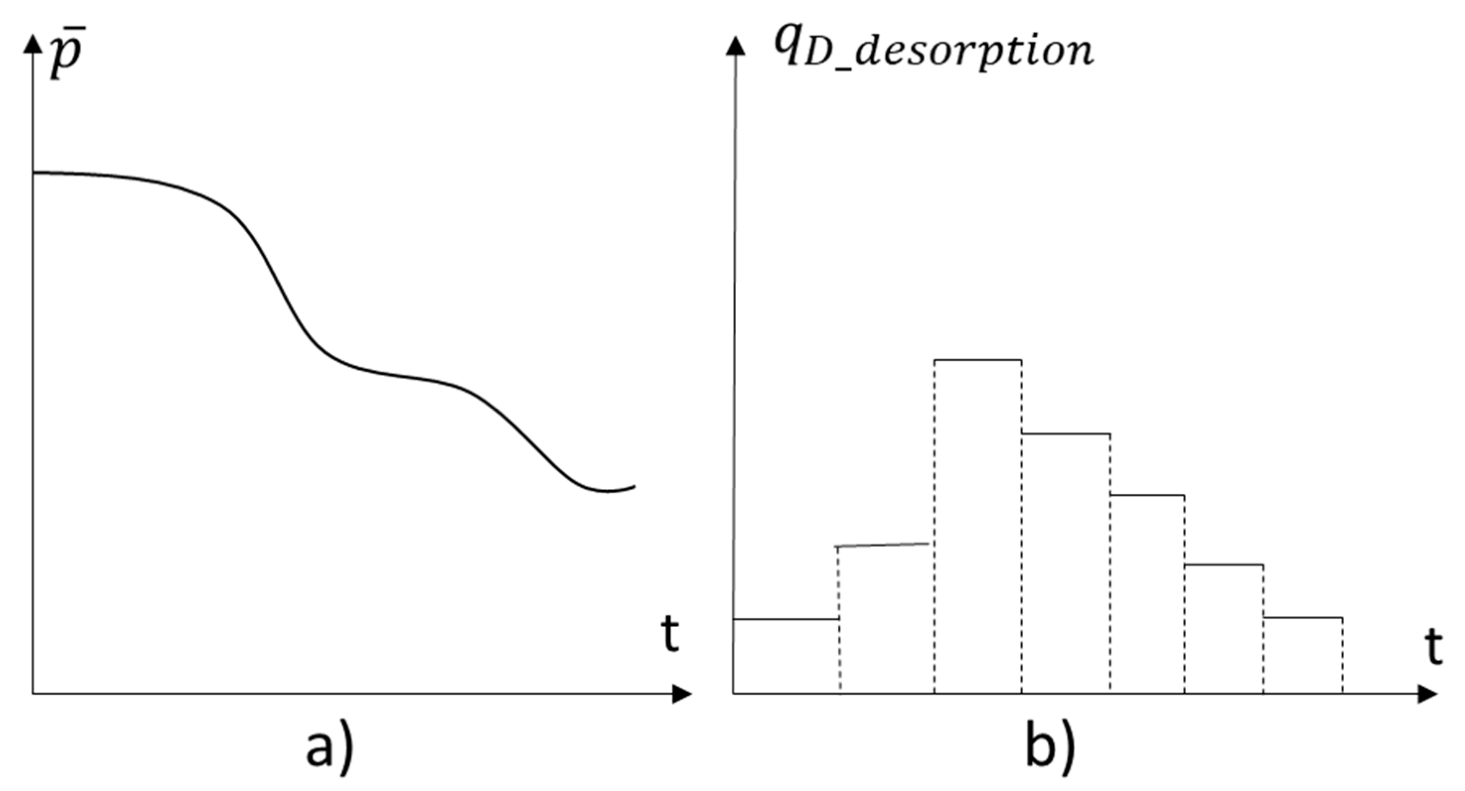
2.2. Desorption Behavior

The gas desorption behavior characterized from lab experiments was used in this analytical model. The widely accepted Langmuir isotherm was used as an example to demonstrate the application of the proposed method in a shale gas desorption analysis. The gas content per unit weight of shale or coal rock can be expressed as follows:

$$C=\frac{V_{L}p}{p_L+p}$$

(16)

where C is the gas content, measured in scf/ton of coal or shale rock; $V_L$ is the Langmuir volume, which is the largest volume of the adsorbed gas per unit weight of rock; and $p_L$ is the critical desorption pressure when the gas content reaches ${0.5V}_L$. The Langmuir volume and pressure are described graphically in Figure 4.

According to the Langmuir model, the desorbed gas due to the pressure change can be mathematically described as follows:

$$∆V=\left(\frac{p_{old}}{p_L+p_{old}}-\frac{p_{new}}{p_L+p_{new}}\right)·V_L$$

(17)

where $∆V$ is the desorbed gas due to the pressure change from $p_{old}$ to $p_{new}$ per unit weight of the rock matrix. Assuming this process takes $∆t$, the gas desorption rate in a specific volume of the reservoir in a 2D system can be mathematically described as follows:

$$q_{desorption}=\frac{∆V}{∆t}=\frac{\left(\frac{{\overline{p}}_{old}}{p_L+{\overline{p}}_{old}}-\frac{{\overline{p}}_{new}}{p_L+{\overline{p}}_{new}}\right)·V_L·{\rho }_b·∆x∆yh}{∆t}$$

(18)

where ${\rho }_b$ is the bulk density, $∆x$ and $∆y$ are the sizes of the specific volume in a 2D system, h is the reservoir thickness, and the “¯” on the variables means the average value in this specific volume.

According to physics, desorbed gas is released naturally into the reservoir when the pressure decreases, adding free gas to the reservoir. This addition of the desorbed gas is equivalent to a free-gas injection from a virtual bulk-shaped injection well. By substituting Equation (18) to Equation (13), the pressure change to the system due to the gas desorption from this specific volume (Figure 5) can be quantified as follows:

$$m_D\left(x_D,y_D,t_D\right)={\int }_0^{t_D}\frac{1}{2}·q_{D\_desorption}\left({\tau }_D\right)·p_{sx}\left(t_D-{\tau }_D\right)·p_{sy}\left(t_D-{\tau }_D\right)d{\tau }_D$$

(19)

where $p_{sx}\left(t_D-{\tau }_D\right)$ and $p_{sy}\left(t_D-{\tau }_D\right)$ are the source/sink functions in the x and y directions, respectively, which can be derived by the integral of the point-source solution along the x and y directions:

$$p_{sx}\left(t_D-{\tau }_D\right)=\frac{1}{∆x}{\sum }_{-\infty }^{\infty }\left\{\frac{1}{2}erf\left[\frac{x_R-x+2n{x}_e}{2\sqrt{t_D-{\tau }_D}}\right]-\frac{1}{2}erf\left[\frac{x_L-x+2n{x}_e}{2\sqrt{t_D-{\tau }_D}}\right]+\frac{1}{2}erf\left[\frac{x_R+x+2n{x}_e}{2\sqrt{t_D-{\tau }_D}}\right]-\frac{1}{2}erf\left[\frac{x_L+x+2n{x}_e}{2\sqrt{t_D-{\tau }_D}}\right]\right\}$$

(20)

$$p_{sy}\left(t_D-{\tau }_D\right)=\frac{1}{∆y}{\sum }_{-\infty }^{\infty }\left\{\frac{1}{2}erf\left[\frac{y_T-y+2n{y}_e}{2\sqrt{t_D-{\tau }_D}}\right]-\frac{1}{2}erf\left[\frac{y_B-y+2n{y}_e}{2\sqrt{t_D-{\tau }_D}}\right]+\frac{1}{2}erf\left[\frac{y_T+y+2n{y}_e}{2\sqrt{t_D-{\tau }_D}}\right]-\frac{1}{2}erf\left[\frac{y_B+y+2n{y}_e}{2\sqrt{t_D-{\tau }_D}}\right]\right\}$$

(21)

where $x_L$, $x_R$, $y_B$, and $y_T$ are the coordinates of the specific volume; $x_e$ and $y_e$ are the boundary locations; and “erf” stands for the error function defined in Equation (22):

$$erf\left(x\right)=\frac{2}{\sqrt{\pi }}{\int }_0^x{e}^{-t^2}dt$$

(22)

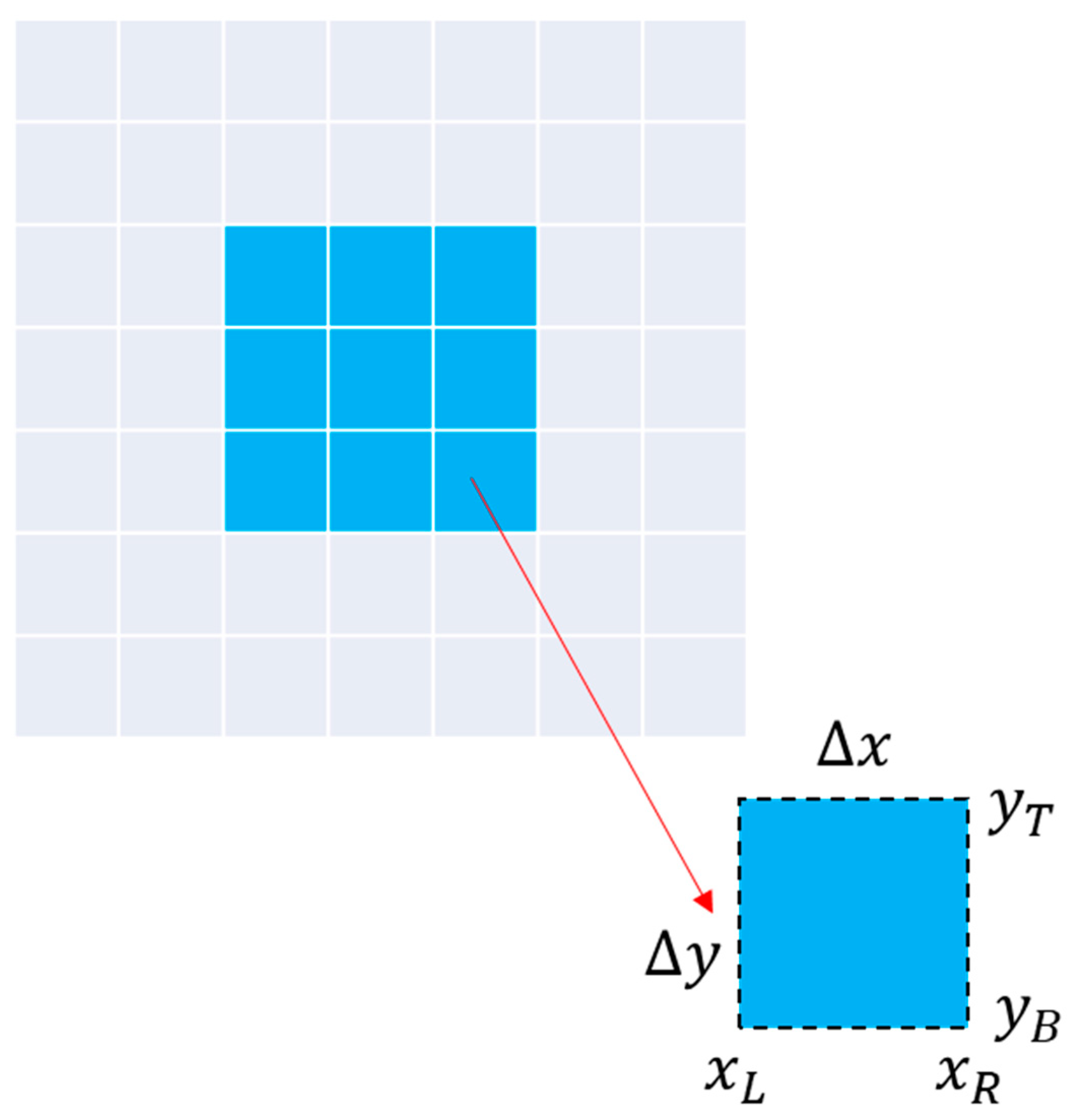
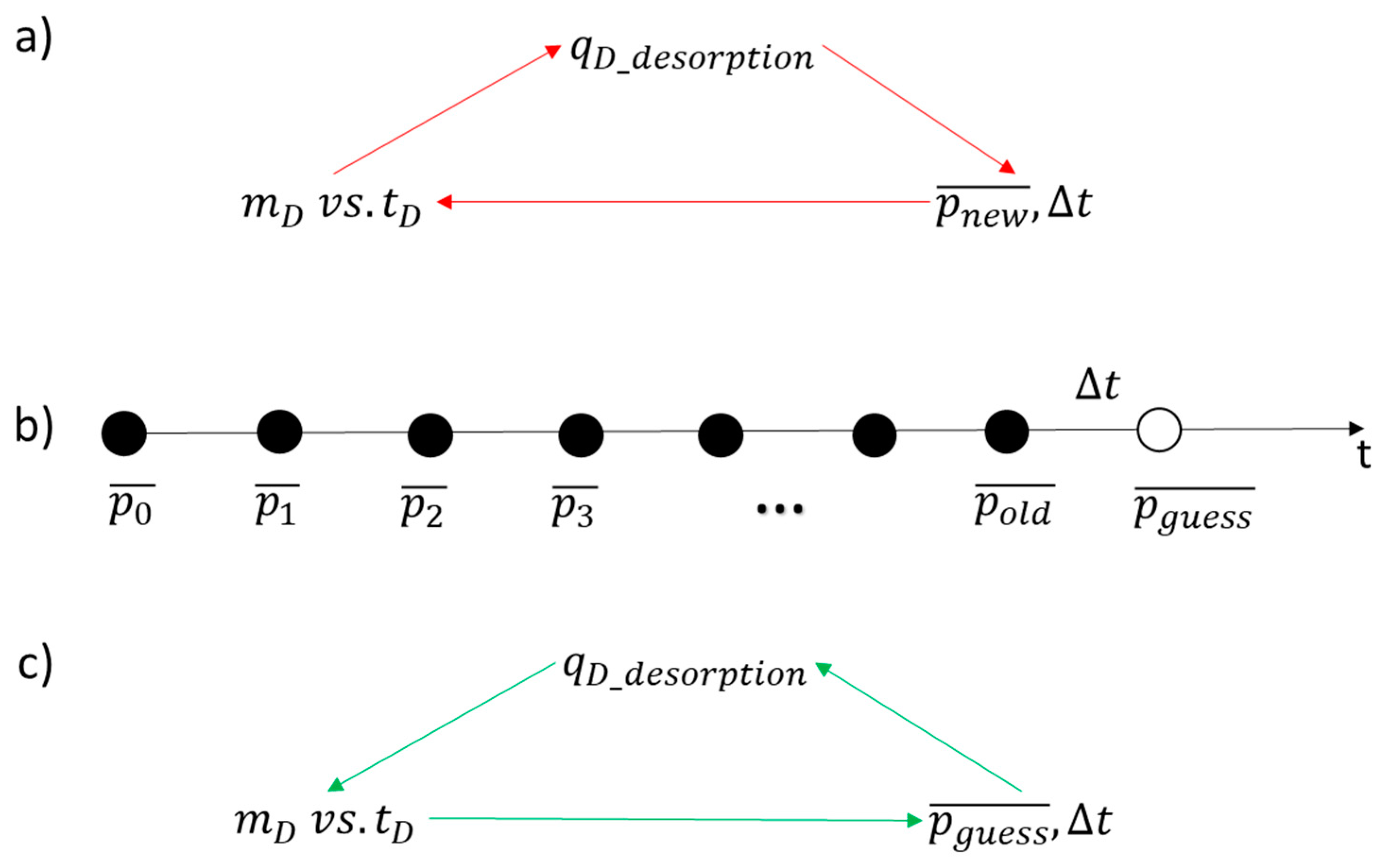
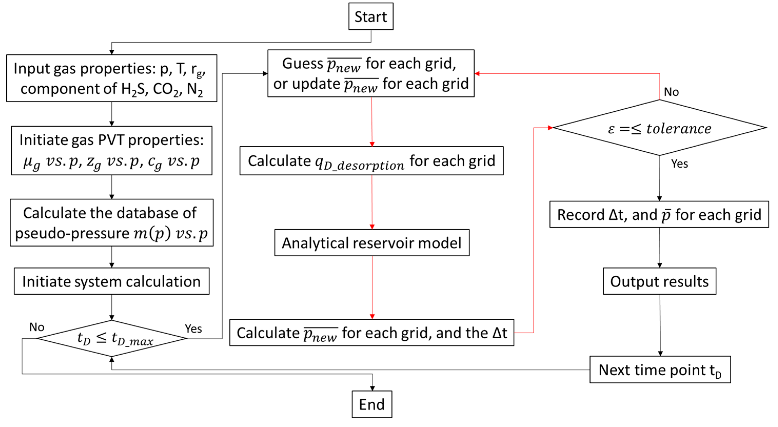
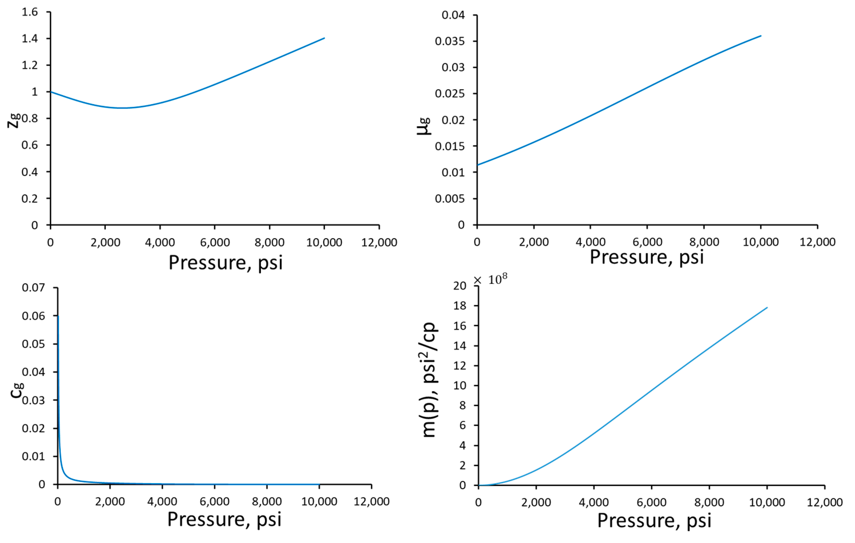
2.3. Non-Linear System

The non-linearity due to the gas desorption from the rock came from two aspects. The gas desorption rate versus time did not have an analytical solution. For example, similar to the system of fluid flows, the change in the pressure in a specific area can be random (Figure 6a). The desorption rate of that area follows the derivative line of the average pressure, which is also non-linear. In order to quantify the desorption rate for the calculation, we assumed that, over a small specific time range, $∆t$, the desorption rate was uniform, as shown in Figure 6b. By further applying the superposition principle, similarly to the well-testing theory, this kind of stepped-rate gas injection problem can be expressed semi-analytically.

The other difficulties came from the unknown pressure at a given time point, because we need the change in pressure to calculate the amount of gas desorbed from the last time point. We can then calculate the overall pressure change if we know the amount of desorbed gas from the last time point, forming a closed circle that cannot be solved analytically (Figure 7a). Here, we introduce a system involving a self-iterative coupling method to solve this problem. In the calculation at the present time point, a guessed input of the average pressure is assumed (Figure 7b) and used to calculate the amount of gas desorbed since the last time point. The calculated desorption rate is then used to calculate the present pressure, updating the previous guessed average pressure value (Figure 7c). The calculation loop will keep running until an acceptable difference between the average pressure values of the two most recent iterations is achieved. The details of the modeling procedures are shown in a flowchart (Figure 8). The calculations of the source/sink functions, the numerical Laplace transformation, the matrix computation, and the inverse Laplace algorithm were all coded using C++ in the Microsoft Visual Studio Community 2022 environment.

The reservoir-scale system modeling was based on a patented reservoir simulation methodology using the integral image method of source-and-sink functions [39]. The source-and-sink functions were calculated at each edge of the sub-grids of the system to capture the accurate cross-boundary flow flux. This method has been successfully applied in the analytical modeling of multistage horizontal fractured wells [40] and many other extended studies [32,41,42].

3. Case Study and Results

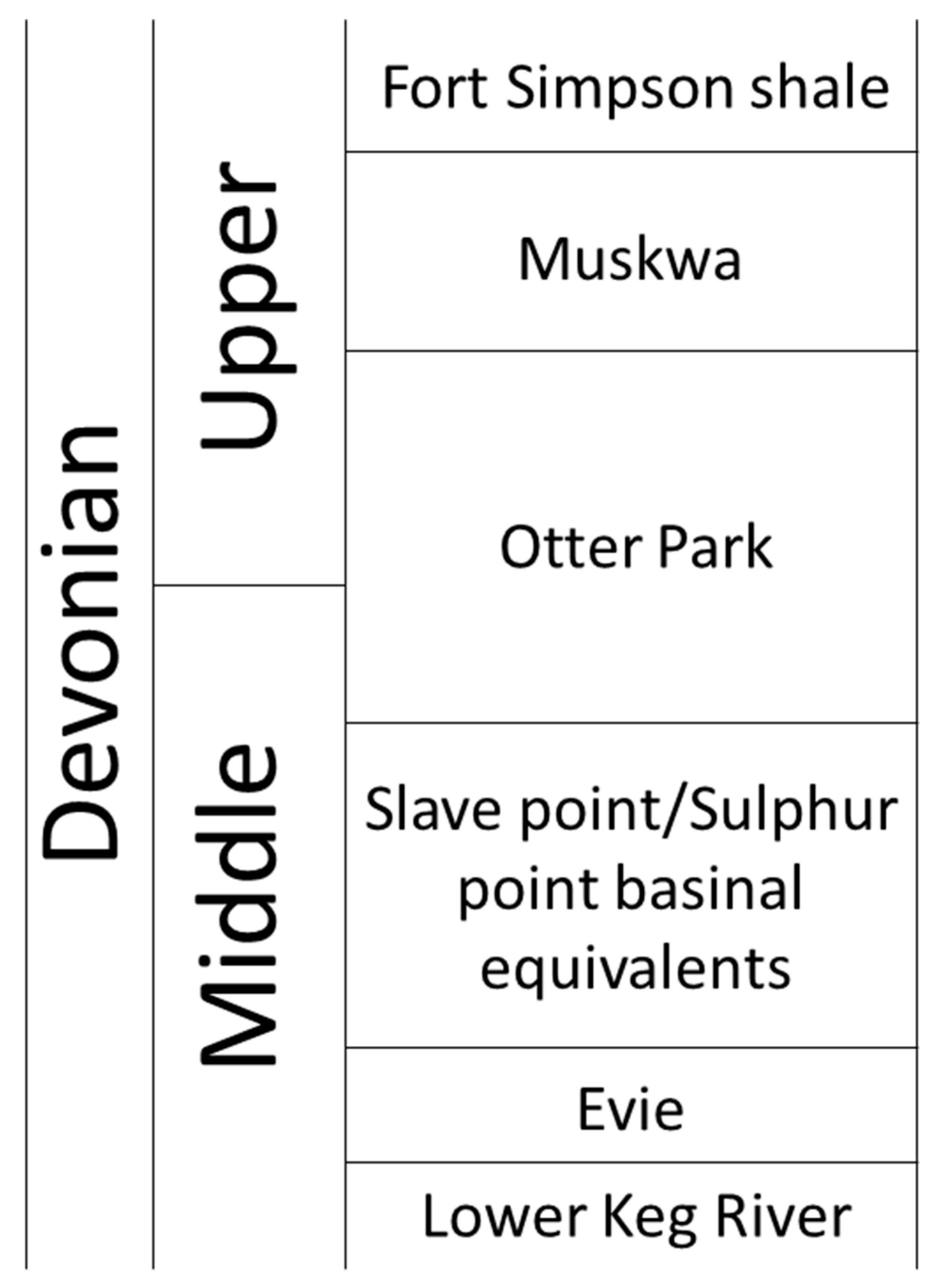
3.1. Reservoir Description

The Horn River shale gas play in the Horn River Basin (HRB), British Columbia, Canada, is one of the major shale gas plays in NE British Columbia, Canada, along with other shale regions, such as the Liard Basin, the Cordova Embayment, and the Montney. Dry natural gas resources [43] are mainly stored in the Muskwa, Otter Park, and Evie formations (Figure 9). A study by Dong et al. [44] showed that this shale reservoir has a complex pore system. Organic-matter-hosted pores, intraparticle pores, and interparticle pores are present in the Horn River shale reservoirs, and they form the porous media for the gas flow. Organic-matter-hosted pores are much smaller than intraparticle and interparticle pores. Although micropores dominate in number, mesopores and macropores contribute more to the total pore volume. Kim et al. [45] conducted a shale gas resource assessment of the Horn River shales and suggested that adsorbed gas accounts for 43% of the initial original gas in place.

The HRB has experienced a period of robust development since 2005 because of the advances in horizontal wellbore drilling and the associated multistage hydraulic fracturing technologies [46]. In 2011, the HRB was estimated to ultimately contain 78 Tcf of marketable gas resources [47]; the peak number of active producing wells in this region reached 222 in 2015, and a large amount of data has been accumulated that could help us better understand the role of gas desorption in production and recovery. However, drilling and production began to slow down due to the unfavorable natural gas price [48]. Although only 99 wells remain in production as of December 2020, a renewal of the development of the natural gas resources in this region can be expected in response to increasing demands for natural gas as a low-carbon energy transition. The general reservoir properties of the HRB are summarized in

Table 1. Horn River shale gas reservoir parameters [43].

Depth Range	1900–3100 m
TOC range	1–5%
Porosity	3–6%
Pressure	20–53 MPa
Pressure regime	Normal-Over Pressure
Temperature	80–160 °C

.

Figure 9. Middle and basal Upper Devonian stratigraphy of the Horn River Basin (modified according to McPhail et al. [49]).

Figure 9. Middle and basal Upper Devonian stratigraphy of the Horn River Basin (modified according to McPhail et al. [49]).

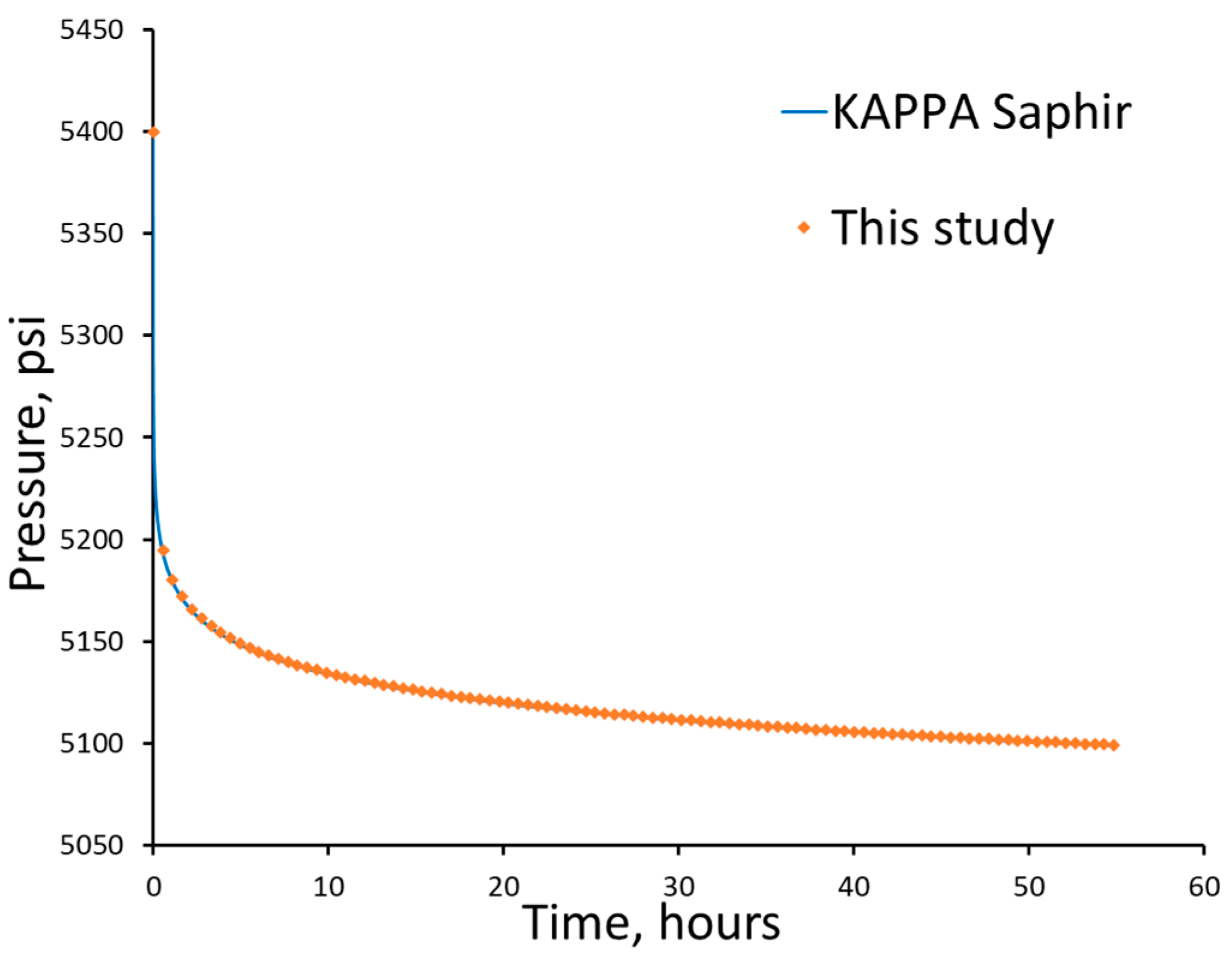
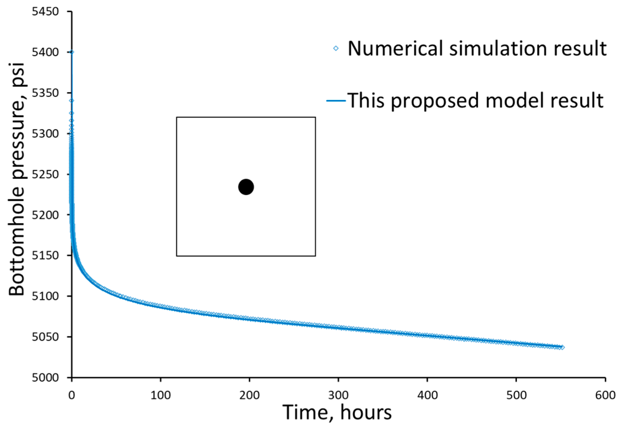
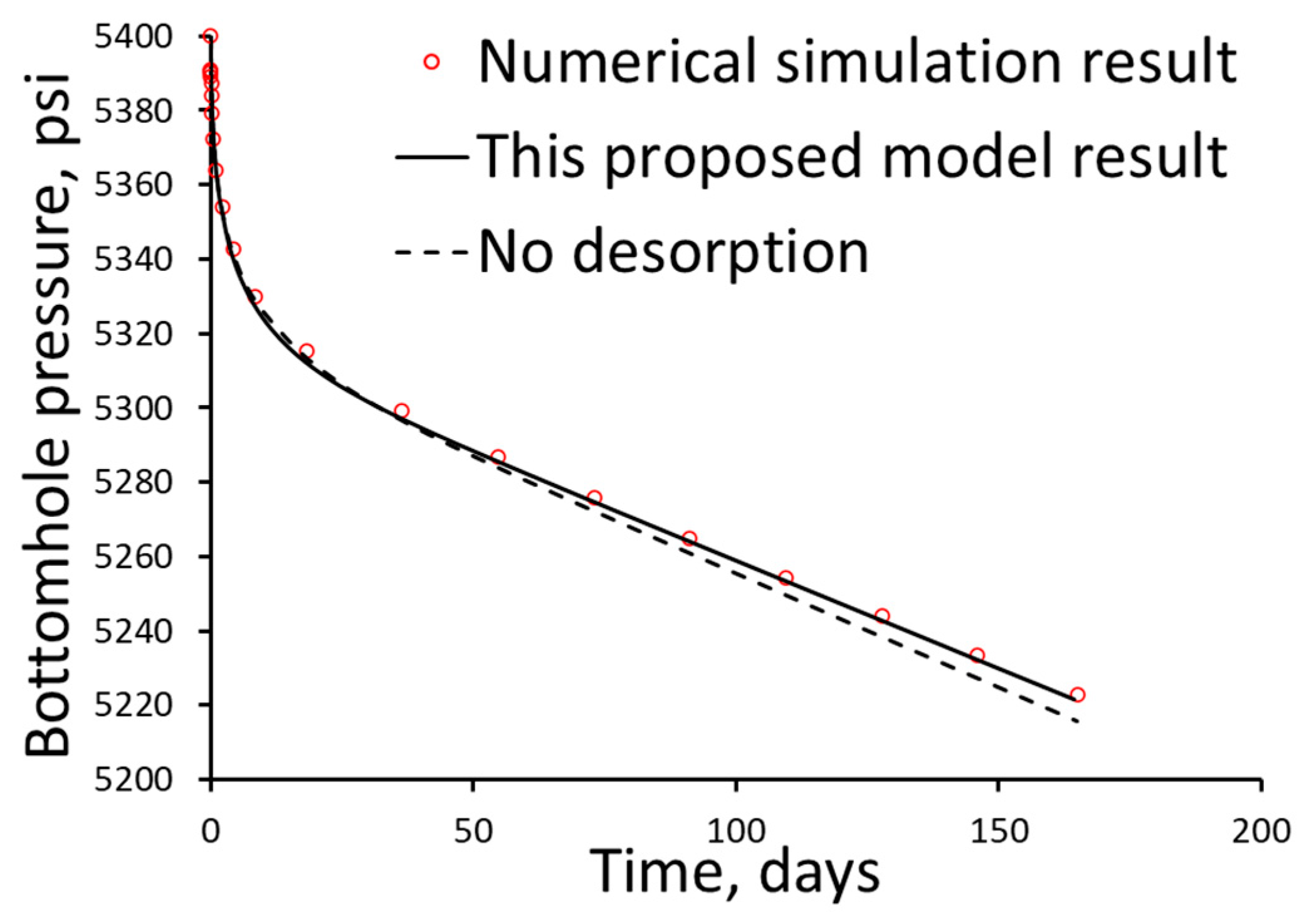
3.2. Production-Well Performance

Two wellbore configurations were studied to analyze the bottomhole pressure variation under a constant gas production rate. Figure 10 shows the vertical and fractured wells in a 2D reservoir system. The reservoir and gas properties remained the same in both well configuration models and are summarized in

Table 2. Parameters of the reservoir and gas used in the case study.

Parameter	Symbol	Value	Unit
Reservoir permeability	k	0.5	md
Reservoir porosity	$\varnothing$	3	%
Reservoir thickness	h	100	ft
Reservoir initial pressure	$p_i$	5400	psi
Reservoir temperature	T	80	°C
Bulk density	${\rho }_b$	0.078	Ton/ft3
Langmuir volume	$V_L$	55	scf/ton
Langmuir pressure	$p_L$	740	psi
Gas specific gravity	${\gamma }_g$	0.6
Production rate at surface	$q_{std}$	1000	Mscf/day

.

The gas-pressure-dependent properties, including the viscosity, compressibility factor, and compressibility, were calculated using classical empirical formulas. However, raw experimental data can also be used in this methodology. The natural gas viscosity was derived from the empirical equation developed by Carr, Kobayashi, and Burrows [50], and the compressibility factor was derived from Brill and Beggs’s z-factor correlation [51]. The details for those empirical equations can be found in the Natural Gas Engineering Handbook [52]. The gas compressibility was calculated using Equation (23). The gas compressibility factor, viscosity, and compressibility are plotted in Figure 11. The numerical integration was then used to obtain the pseudo-pressure (Figure 11), which was inversed to the real pressure value.

$$c_g=\frac{1}{p}-\frac{1}{z_g}\frac{\partial z_g}{\partial p}$$

(23)

Figure 12 shows the bottomhole pressure decay of the vertical wellbore case in the first 500 h under a constant production rate. The wellbore had a radius of 0.3 ft. The downhole wellbore pressure dropped sharply from the reservoir’s initial pressure, 5400 psi, to 5100 psi within the first 100 h. Then, it gradually decreased to 5050 psi over the rest of the 400 h. The blue line in the plot represents the results of this study, and the blue circles represent the results of the commercial numerical simulation software, the KAPPA Workstation numerical module V.5.50 (Rubis). The results were clearly well matched in this case.

Figure 13 compares the results of this study with a no-desorption case using the same input parameters. The solid line represents the bottomhole pressure when considering desorption, calculated in this study, and the dashed line represents the pressure without the desorption mechanism. There was no difference between the two cases in the first few hours. However, the difference became evident after 300 h of production. The difference would become larger after years of production. Moreover, a shale gas reservoir with adsorbed gas would provide a higher wellbore pressure under the same production rate. The desorbed gas released from the rock matrix played the role of an additional gas source supply and ensured the maintenance of the reservoir pressure.

The dimensionless results of the pressure derivative are plotted in Figure 14. In well-testing engineering, a log–log plot of the pressure derivative curve helps evaluate the flow regime and diagnose the well’s performance. The solid line represents the results of the shale gas reservoir with the desorption mechanism calculated by this model. The dashed line is the standard conventional gas reservoir without desorption, as the reference line. The dashed line remained at 0.5 before t_D = 2, and then it rose in a straight line. The flat pressure derivative in the log–log plot represents a radial flow regime. At last, the dashed line became a unit slope line, which means that the transient pressure wave reached the boundary of the reservoir, representing the dominant boundary flow. The solid line also started at 0.5, and then gradually dropped slightly below the 0.5 horizontal line. Then, it slowly rose to the unit 1 slope line. However, the values were smaller compared to those of the no-desorption case. In well testing, when the pressure derivative value becomes lower, it usually means that the transient pressure wave reached a better reservoir, such as a reservoir with a higher permeability and porosity. In contrast, when the pressure derivative value increases, it could mean that the transient pressure wave met an obstruction, such as a lower-permeability region, a boundary, or a sealed fault. In this standard case for a shale gas reservoir with gas desorption, the pressure derivative started with a radial flow. However, because of the release of additional gas, the pressure derivative decreased. At last, it still reached the boundary as a unit slope line, but the pressure derivative value was lower than in the no-desorption case. As such, a dimensionless pressure derivative plot could be potentially used to compare different shale gas plays for gas adsorption.

In this study, variable reservoir discretization was used to handle the spatial variation in gas desorption in the reservoir. The model grid was denser near the production wellbore, where the greatest pressure drop occurred and the desorbed gas accumulated the most. Usually, in numerical simulations, finer gridding is needed to obtain an accurate result. Figure 15 shows the results of this study, where various grid numbers were used to test the accuracy. The bottomhole pressure resulted in overlap, which showed a good accuracy for this methodology.

The images on the left-hand side of Figure 16 show the 2D meshed pressure distributions at three different time points. The transient pressure wave moving towards the boundary was identified. At t_D = 0.5, it showed a radial flow region. When t_D = 4, it was in the transition zone from a radial flow to a dominant boundary flow. It reached the boundary when t_D = 10. The other three images on the right-hand side of the figure are the 3D plots of the pressure distribution at the same three time points. The pressure drop started from the center wellbore. After 9 days, the pressure across the entire reservoir was below the initial reservoir pressure, and it kept decreasing below 5370 psi after 23 days.

The case of a fractured wellbore was also studied. The half-length of the fracture was 300 ft, and it was located in the center of the system. Figure 17 shows the dimensionless pressure derivative curve of the cases that did and did not consider adsorption. The black solid line is the pressure derivative curve without considering desorption, as the baseline for comparison. The green dashed line is the case that did consider gas desorption. The black line started as a half-slope line, which indicates that it was in the linear flow regime. Then, it gradually increased to a flat line at a value of 0.5, which shows a radial flow. Eventually, it kept increasing and became a unit slope line, which shows that the pressure wave reached the boundary and entered the dominant boundary flow. The green dashed line also started as a half-slope line. However, in the middle of the transition zone, it was lower than that for the no-desorption case, and when it eventually reached the dominant boundary flow, the values were smaller than those for the no-desorption case. This also demonstrates that the desorbed gas acted as an additional source to strengthen the gas flow in production. In addition, the desorption ability could be identified from the difference.

The wellbore pressure is plotted in Figure 18 and compared to the results without consideration of desorption behavior. The pressure dropped from 5400 psi to 5220 psi in the 160-day period and was higher than that in the model that did not consider gas desorption. The results from the proposed method matched well with the numerical simulation output, with a high calculation accuracy.

In the fracture modeling, the total fracture was further divided into 50 sub-segments. Each segment had a uniform, but transient, gas influx distribution. Five typical times were chosen to show the influx difference at the different locations within the fracture (Figure 19). In general, the segments near the edge had a higher flux rate because they were less affected by the interference effect from other nearby segments. From the time domain aspect, the flux rates were nearly the same in the very early stages. However, with the continuous influence of the interference, the segments in the middle area lost their gas production ability, while the flux rates of the segments near the edge increased.

In contrast to the results for the vertical wellbore, the shape of the pressure distribution of the fractured well was similar to an oval (Figure 20). The pressure drop occurred along the fracture and then spread out to the reservoir. Due to the more vital gas production ability of the fractured well, the bottomhole pressure drop was not as significant as that of the vertical wellbore. When t_D = 0.1, the flow regime was in the transition zone from linear to radial flow. Therefore, the pressure change front exhibited a near-rectangular shape, with thicker parts in the middle. When t_D = 1, it was in the radial flow, and the transient pressure front displayed a circular shape. When t_D = 10, the pressure change reached the boundary, and the overall reservoir pressure decreased at the same rate.

4. Sensitivity Discussion

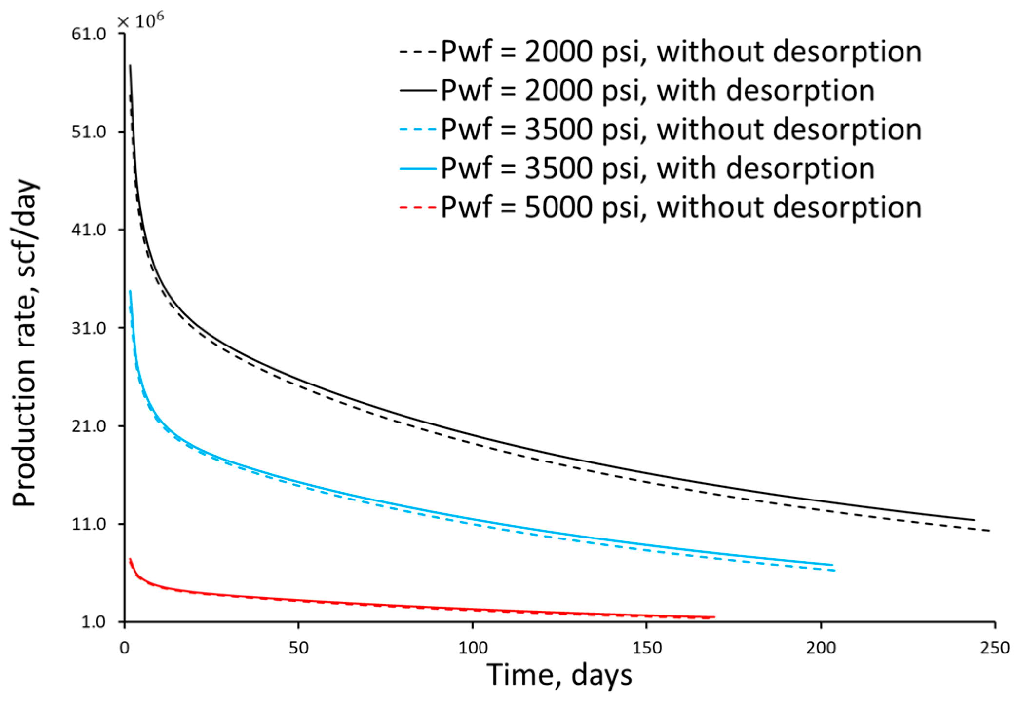
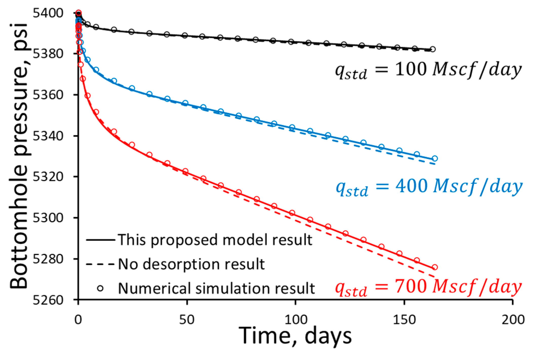
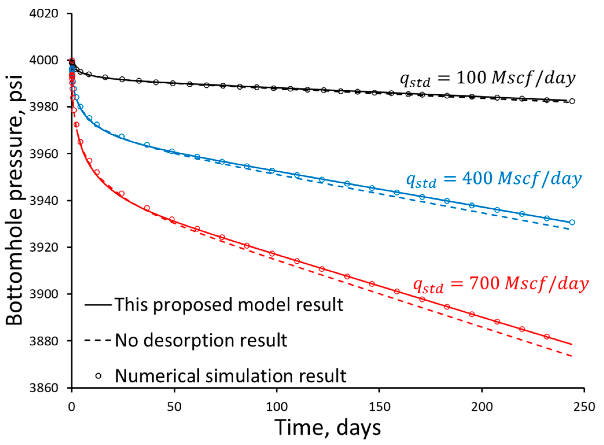
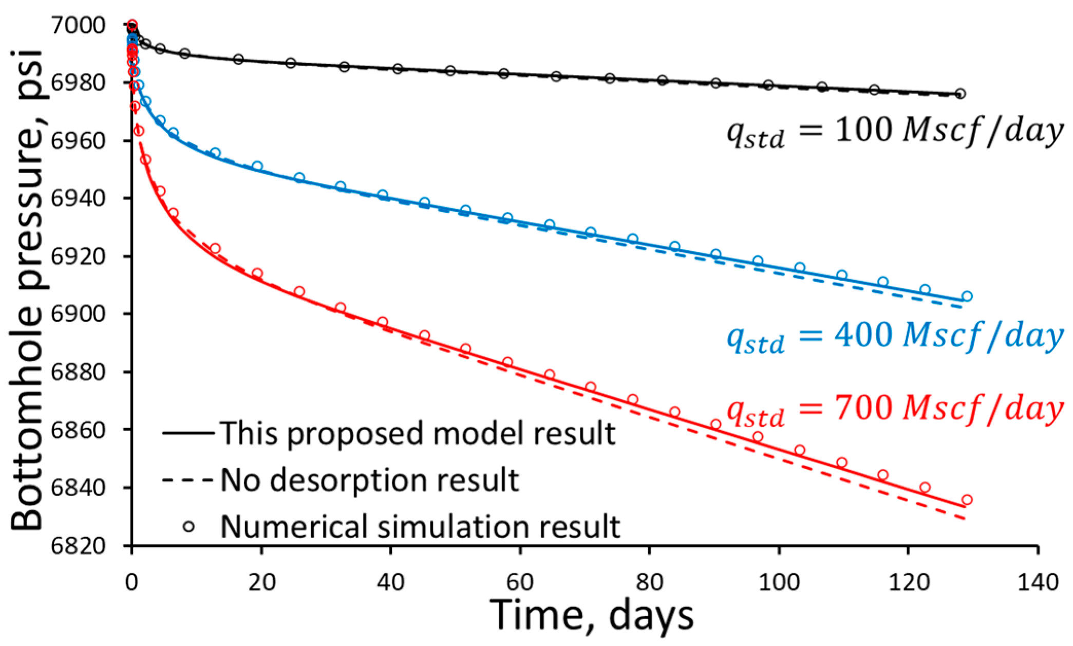
4.1. Various Bottomhole Pressures

The production rates under various constant bottomhole pressure values were calculated and are plotted in Figure 21. The associated cases without considering gas desorption behavior are also plotted for comparison. A lower pressure (a higher pressure difference compared to the reservoir pressure) led to higher gas production rates. When the wellbore pressure was 5000 psi, a difference between the cases that did and did not consider gas desorption was not apparent. The adsorbed gas amount was minimal to show the difference. When the wellbore pressure was 2000 psi, a significant pressure drop occurred in the near-wellbore region. A large amount of desorbed gas was released, thus supplying the free-gas flow. The production was maintained at a higher level. The difference is obvious in Figure 21. In future CCUS applications, a larger CO₂ injection rate could be achieved under the same injection pressure in a reservoir with gas adsorption behavior, which means that shale gas reservoirs and coal beds have good potential for storing CO₂.

4.2. Various Gas Reservoirs and Producing Rates

In order to validate and test the proposed methodology in various reservoirs with different gas properties, three case studies were conducted in a fractured well system. Case A was the base case, with the same values as those of previous studies. Case B had a lower specific gravity, of 0.56, which was close to that of a pure methane reservoir. It had a lower reservoir temperature and initial pressure. Case C had a higher specific gravity, of 0.8, with a higher reservoir temperature and initial pressure, which represents a high-temperature and high-pressure reservoir. The key parameters are listed in

Table 3. Parameters of three case studies, representing different reservoir and gas properties.

	Case A	Case B	Case C
Specific gravity	0.6	0.56	0.8
Temperature, T	80 °C	60 °C	100 °C
Pressure, pi	5400 psi	4000 psi	7000 psi

.

Calculations were applied to the three cases using the methodology proposed in this study and the commercial numerical software KAPPA Workstation Rubis V.5.50. The gridding of the reservoir is shown in Figure 22. The methodology proposed in this study used a simple 5 × 5 grid for the simulation, while the numerical software used a total of 3255 grids, with finer gridding blocks near the fractured wellbore. The modeling comparison between this study and the commercial software aimed to validate the accuracy of the proposed method under three different initial gas reservoir conditions. Using a single fracture in the well added a certain complexity to the well setup, which also tested the gridding effect around the well. However, since the reservoir’s geological setup and the fluid composition are not complicated, the proposed analytical method will be tested further under more heterogeneous and complex fracture-network geo-systems in the future.

Each case was tested by applying three different production rates (Figure 23). A higher production rate led to a quicker and more significant production well pressure drop. When the production rate was lower, such as 100 Mscf/day, the difference between the cases that did and did not consider gas desorption was not evident from the plots. However, the difference was significant when the production rate was higher. More desorbed gas was released from the pore surface of the rock, thus maintaining the reservoir pore pressure. The results from this proposed semi-analytical methodology and the commercial numerical simulation software matched well.

Figure 24 and Figure 25 show the wellbore pressures of Case B and Case C under the same three constant production rates. Case B had a lower initial reservoir pressure and temperature, and Case C had the highest initial pressure and temperature. A higher production rate showed a clear contribution of the desorbed gas to the free-gas flow supply. All three cases used the same Langmuir isotherm parameters. Case B, with an initial reservoir pressure of 4000 psi, was closer to the Langmuir pressure, at 740 psi. More desorbed gas was released under the same pressure drops. As a result, the contribution of desorbed gas was more obvious in Case B. For developing a high initial pressure in the reservoir, higher production rates are better for activating the gas desorption behavior and enhancing the natural gas production.

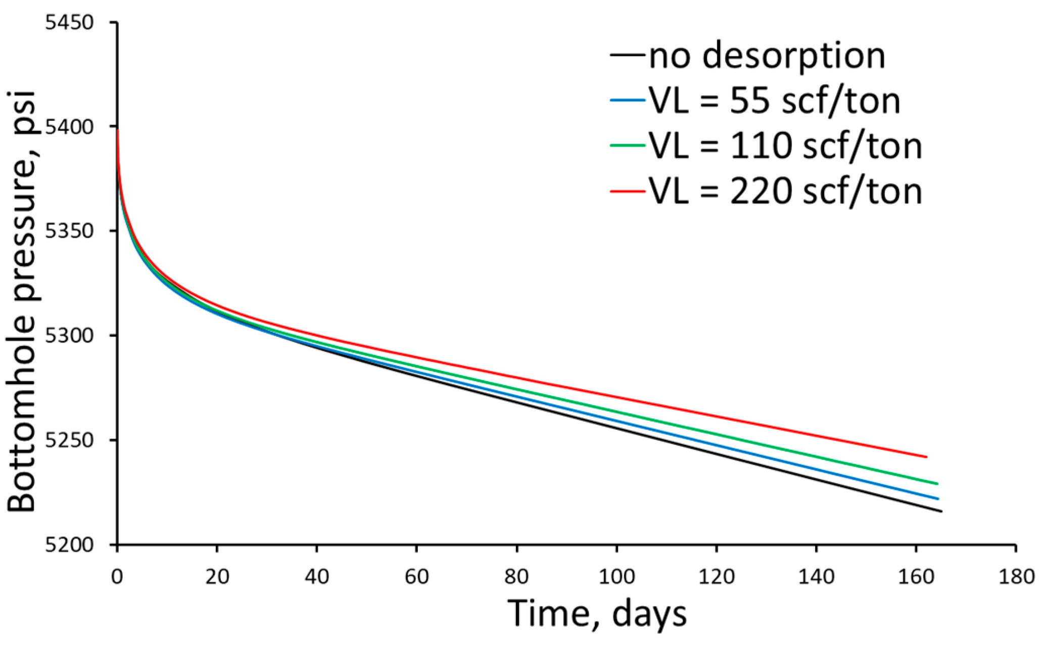
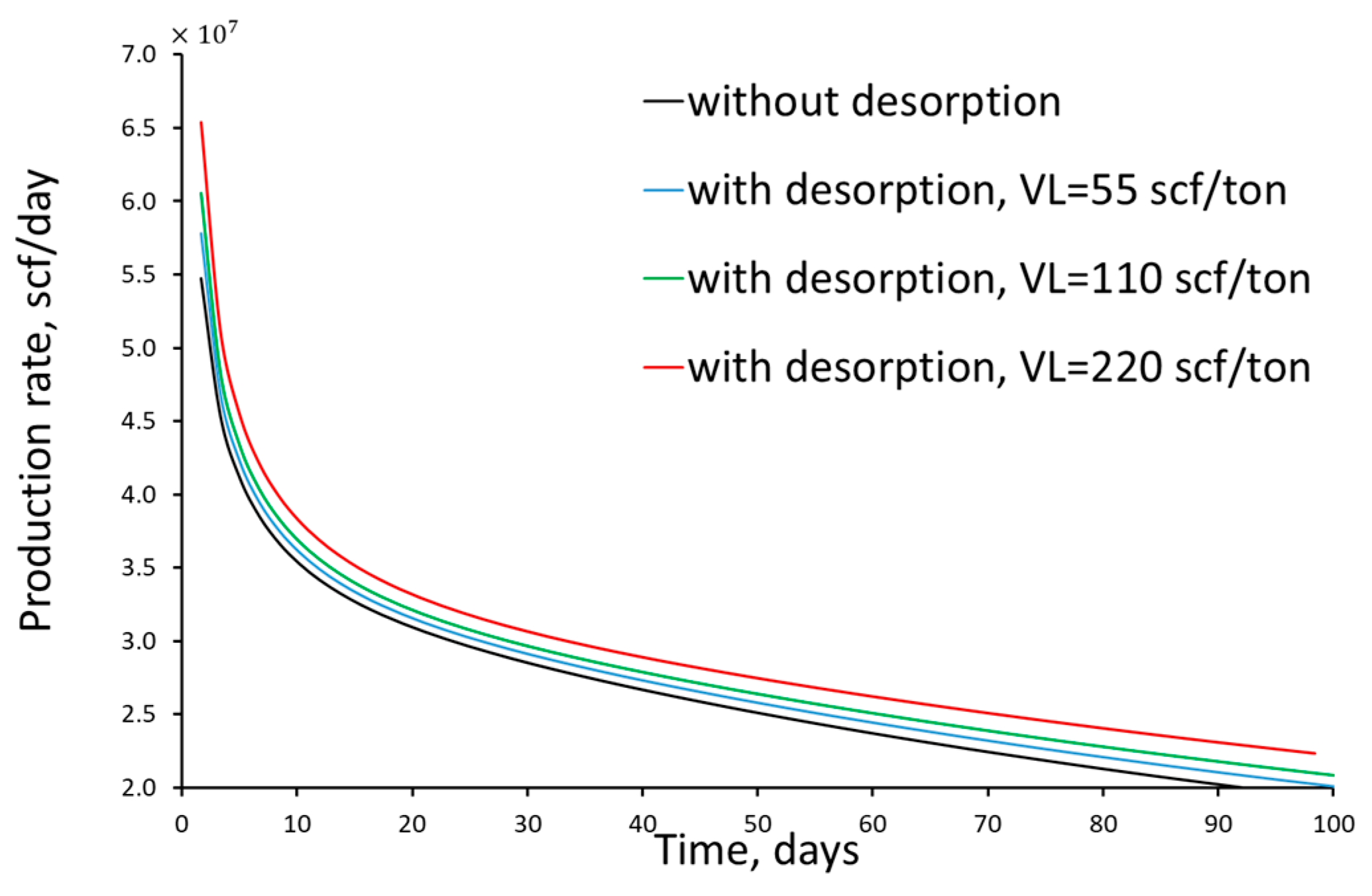
4.3. Various Gas Desorption Abilities (Langmuir Volume)

The Langmuir volume is an important property that needs to be considered for shale gas reservoirs, as it determines the amount of gas adsorbed per unit weight of rock. Figure 26 shows the bottomhole pressure drops from reservoirs with three different Langmuir volumes under the same production rates (1000 Mscf/day). The case with a value of 220 scf/ton V_L had the highest production pressure. For the production, a higher V_L can contribute to a higher gas production rate under the same bottomhole pressure (Figure 27). When using conventional well-testing methods or numerical history matching, a higher production rate or pressure may lead to a higher permeability estimation. Further research on using the pseudo-permeability to replace the desorption behavior in resource assessments is worthwhile to simplify the modeling.

5. Conclusions

This study proposed a semi-analytical methodology to capture the natural gas desorption processes in reservoirs for production modeling. The gas desorption was treated as an additional source/sink term in the system and was handled mathematically using source-and-sink functions. The desorbed gas source term and pressure-dependent gas properties, such as the viscosity and compressibility factor, increased the non-linearity of the gas diffusion in the porous media. Pseudo-terms, an average pressure evaluation, and a self-iterative method were used to linearize the system and solve the problem semi-analytically. Numerical models based on a Horn River Basin shale gas reservoir were constructed to validate the proposed methods and demonstrate the application of the semi-analytical model in predicting the performance of natural gas production while considering gas desorption. A comparison of the results from the proposed methods with those from the commercial fine-gridding numerical simulation software showed good matches with a high accuracy. The major outcomes of this modeling are summarized below:

(1)

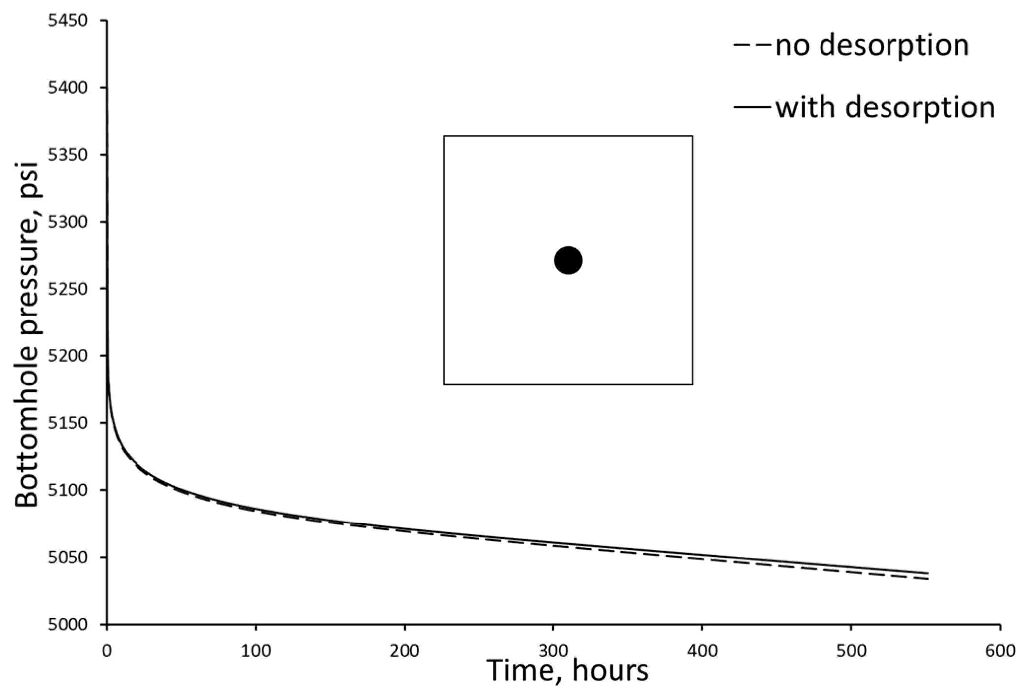
The gas released from the organic-rich shale reservoir added free gas to the reservoir and slowed down the pressure depletion to a certain degree, for instance, by increasing the gas productivity and enhancing the gas recovery;

(2)

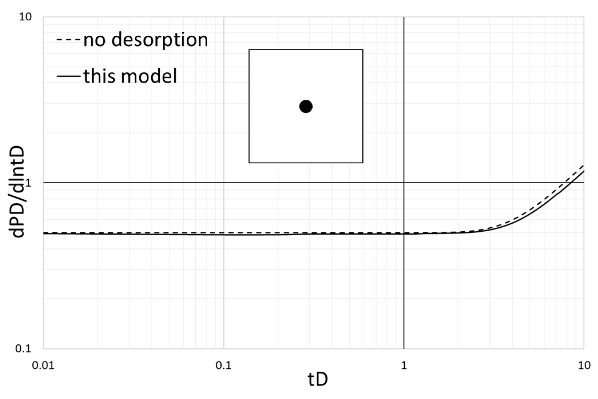
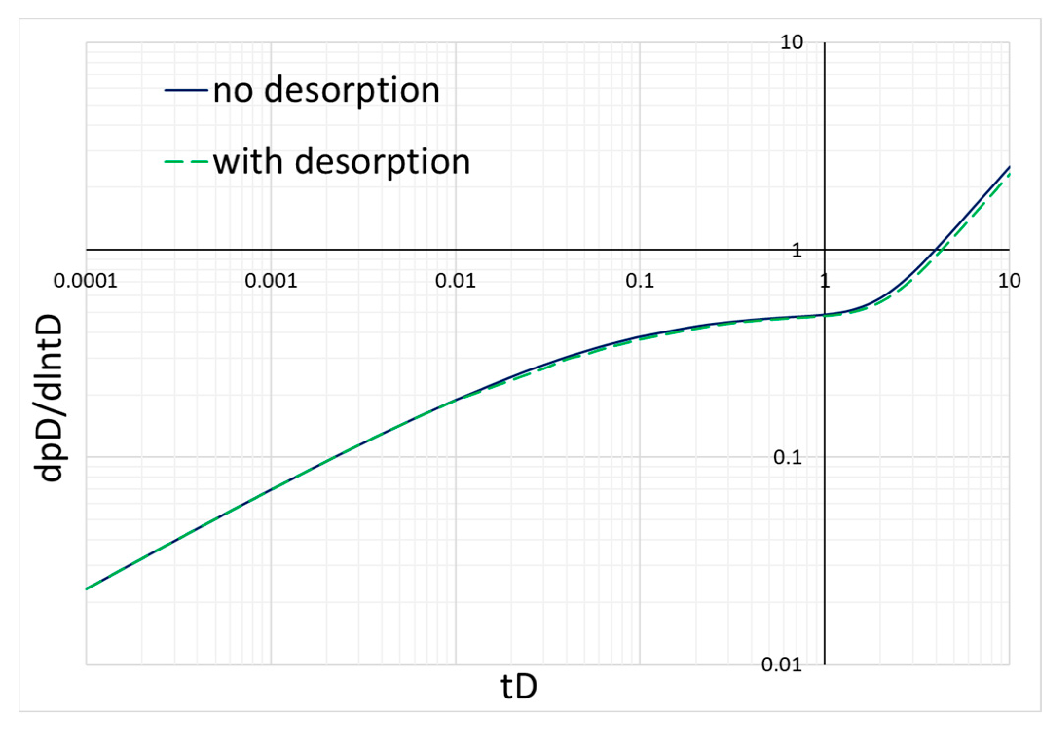
The dimensionless pressure derivative plot could be a potential indicator of gas desorption in comparing different shale gas plays;

(3)

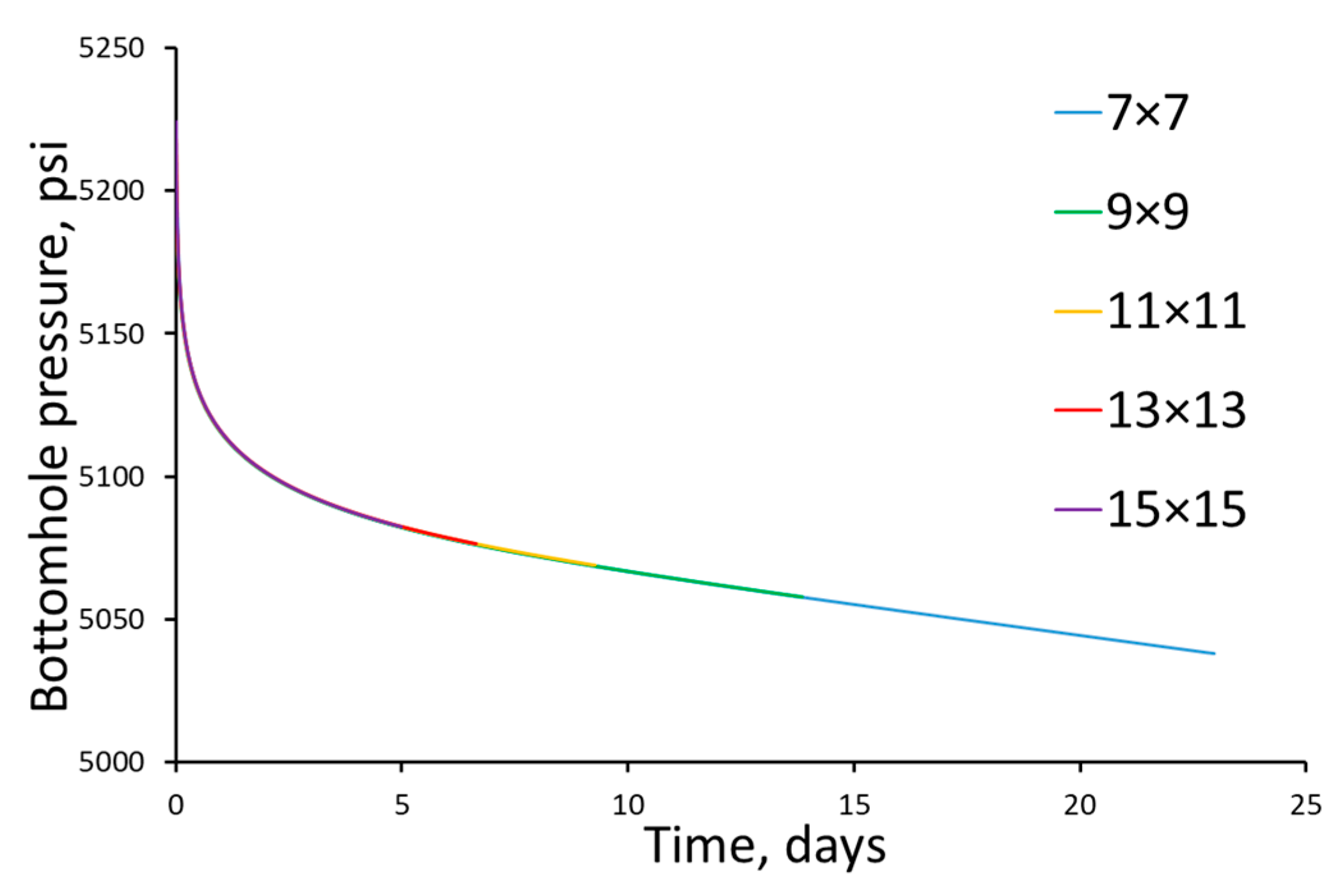
The proposed semi-analytical modeling methodology provides an additional tool for modeling shale gas production while considering gas desorption, with a higher accuracy and computational efficiency;

(4)

Through a preliminary sensitivity analysis, it was found that a lower bottomhole pressure and a high production rate will induce a severe gas desorption mechanism, which will maintain a high production rate and bottomhole pressure. Shale reservoirs with a higher amount of adsorption will have a stronger ability to achieve a high production rate and bottomhole pressure. Through the results and associated dimensionless type curves, the shale gas reservoir desorption ability was roughly diagnosed, which could be very helpful for further resource assessments.

This study mainly focused on realizing the new idea of modeling the desorbed gas in shale reservoirs. Many future works are planned and also recommended for researchers to explore. More detailed sensitivity analyses need to be conducted on more complicated cases of geological and fluid-phase behaviors. For instance, geological heterogeneity and complex fracture networks will significantly affect the pressure decay regime and area, which will further affect the gas flow and the associated desorption behavior. When applying this methodology to condensate shale reservoirs, such as the Duvernay Formation in Canada, the complexity of the gas-phase behavior needs to be considered and integrated into the modeling and sensitivity analysis.

References

1. U.S. Energy Information Administration (EIA). Natural Gas and the Environment. 2021. Available online: https://www.eia.gov/energyexplained/natural-gas/natural-gas-and-the-environment.php (accessed on 20 December 2023).
2. Kazmi, B.; Haider, J.; Taqvi, S.A.A.; Qyyum, M.A.; Ali, S.I.; Awan, Z.U.H.; Lim, H.; Naqvi, M.; Naqvi, S.R. Thermodynamic and economic assessment of cyano functionalized anion based ionic liquid for CO2 removal from natural gas integrated with, single mixed refrigerant liquefaction process for clean energy. Energy 2022, 239, 122425. [Google Scholar] [CrossRef]
3. Jin, Z.; Zhang, J.; Tang, X. Unconventional natural gas accumulation system. Nat. Gas Ind. B 2022, 9, 9–19. [Google Scholar] [CrossRef]
4. Zheng, Y.; Liu, J.; Liu, Y.; Shi, D.; Zhang, B. Experimental Investigation on the Stress-Dependent Permeability of Intact and Fractured Shale. Geofluids 2020, 2020, e8897911. [Google Scholar] [CrossRef]
5. Korre, A.; Shi, J.-Q.; Imrie, C.; Durucan, S. Modelling the uncertainty and risks associated with the design and life cycle of CO2 storage in coalbed reservoirs. Energy Procedia 2009, 1, 2525–2532. [Google Scholar] [CrossRef]
6. van Bergen, F.; Tambach, T.; Pagnier, H. The role of CO2-enhanced coalbed methane production in the global CCS strategy. Energy Procedia 2011, 4, 3112–3116. [Google Scholar] [CrossRef]
7. Prabu, V.; Mallick, N. Coalbed methane with CO2 sequestration: An emerging clean coal technology in India. Renew. Sustain. Energy Rev. 2015, 50, 229–244. [Google Scholar] [CrossRef]
8. Jiang, K.; Ashworth, P. The development of Carbon Capture Utilization and Storage (CCUS) research in China: A bibliometric perspective. Renew. Sustain. Energy Rev. 2021, 138, 110521. [Google Scholar] [CrossRef]
9. Kou, Z.; Zhang, D.; Chen, Z.; Xie, Y. Quantitatively determine CO2 geosequestration capacity in depleted shale reservoir: A model considering viscous flow, diffusion, and adsorption. Fuel 2022, 309, 122191. [Google Scholar] [CrossRef]
10. Yutong, F.; Yu, S. CO2-adsorption promoted CH4-desorption onto low-rank coal vitrinite by density functional theory including dispersion correction (DFT-D3). Fuel 2018, 219, 259–269. [Google Scholar] [CrossRef]
11. Mao, L.; Zhang, Z. Transient temperature prediction model of horizontal wells during drilling shale gas and geothermal energy. J. Pet. Sci. Eng. 2018, 169, 610–622. [Google Scholar] [CrossRef]
12. Renaud, E.; Weissenberger, J.A.; Harris, N.B.; Banks, J.; Wilson, B. A reservoir model for geothermal energy production from the Middle Devonian Slave Point Formation. Mar. Pet. Geol. 2021, 129, 105100. [Google Scholar] [CrossRef]
13. Grasby, S.E.; Allen, D.M.; Bell, S.; Chen, Z.; Ferguson, G.; Jessop, A.; Kelman, M.; Ko, M.; Majorowicz, J.; Moore, M.; et al. Geothermal Energy Resource Potential of Canada; Geological Survey of Canada, Open File 6914; Natural Resources Canada: Ottawa, ON, Canada, 2011; 322p. [CrossRef]
14. Ambrose, R.J.; Hartman, R.C.; Diaz-Campos, M.; Akkutlu, I.Y.; Sondergeld, C.H. Shale gas-in place calculations Part I: New pore-scale considerations. SPE J. 2012, 17, 219–229. [Google Scholar] [CrossRef]
15. Chen, Z.; Lavoie, D.; Malo, M.; Jiang, C.; Sanei, H.; Ardakani, O.H. A dual-porosity model for evaluating petroleum resource potential in unconventional tight-shale plays with application to Utica Shale, Quebec (Canada). Mar. Pet. Geol. 2017, 80, 333–348. [Google Scholar] [CrossRef]
16. Wang, J.; Luo, H.; Liu, H.; Cao, F.; Li, Z.; Sepehrnoori, K. An integrative model to simulate gas transport and production coupled with gas adsorption, non-Darcy flow, surface diffusion, and stress dependence in organic-shale reservoirs. SPE J. 2018, 22, 244–264. [Google Scholar] [CrossRef]
17. Das, J. Extracting Natural Gas through Desorption in Shale Reservoirs. SPE JPT. The Way Ahead. 2012. Available online: https://jpt.spe.org/twa/extracting-natural-gas-through-desorption-shale-reservoirs (accessed on 20 December 2023).
18. Yu, W.; Sepehrnoori, K.; Patzek, T.W. Modeling Gas Adsorption in Marcellus Shale With Langmuir and BET Isotherms. SPE J. 2016, 21, 589–600. [Google Scholar] [CrossRef]
19. Sang, Y.; Chen, H.; Yang, S.; Guo, X.; Zhou, C.; Fang, B.; Zhou, F.; Yang, J. A new mathematical model considering adsorption and desorption process for productivity prediction of volume fractured horizontal wells in shale gas reservoirs. J. Nat. Gas Sci. Eng. 2014, 19, 228–236. [Google Scholar] [CrossRef]
20. Pang, W.; Wang, Y.; Jin, Z. Comprehensive Review about Methane Adsorption in Shale Nanoporous Media. Energy Fuels 2021, 35, 8456–8493. [Google Scholar] [CrossRef]
21. Hildenbrand, A.; Krooss, B.M.; Busch, A.; Gaschnitz, R. Evolution of methane sorption capacity of coal seams as a function of burial history e a case study from the Campine Basin, NE Belgium. Int. J. Coal Geol. 2006, 66, 170–203. [Google Scholar] [CrossRef]
22. Zhang, T.; Ellis, G.S.; Ruppel, S.C.; Milliken, K.; Yang, R. Effect of organic-matter type and thermal maturity on methane adsorption in shale-gas systems. Org. Geochem. 2012, 47, 120–131. [Google Scholar] [CrossRef]
23. Liu, D.; Yuan, P.; Liu, H.; Li, T.; Tan, D.; Yuan, W.; He, H. High-pressure adsorption of methane on montmorillonite, kaolinite and illite. Appl. Clay Sci. 2013, 85, 25–30. [Google Scholar] [CrossRef]
24. Rexer, T.F.T.; Benham, M.J.; Aplin, A.C.; Thomas, K.M. Methane adsorption on shale under simulated geological temperature and pressure conditions. Energy Fuels 2013, 27, 3099–3109. [Google Scholar] [CrossRef]
25. Ross, D.J.K.; Bustin, R.M. The importance of shale composition and pore structure upon gas storage potential of shale gas reservoirs. Mar. Pet. Geol. 2009, 26, 916–927. [Google Scholar] [CrossRef]
26. Jarvie, D.M. Shale resource systems for oil and gas: Part 1—shale-gas resource systems. In Shale Reservoirs-Giant Resources for the 21st Century: AAPG Memoir 97; Breyer, J.A., Ed.; AAPG: Tulsa, OK, USA, 2012; pp. 69–87. [Google Scholar]
27. Gao, X.; Liu, L.; Jiang, F.; Wang, Y.; Xiao, F.; Ren, Z.; Xiao, Z. Analysis of geological effects on methane adsorption capacity of continental shale: A case study of the Jurassic shale in the Tarim Basin, northwestern China. Geol. J. 2016, 51, 936–948. [Google Scholar] [CrossRef]
28. Lee, W.J.; Holditch, S.A. Application of pseudotime to buildup test analysis of low-permeability gas wells with long-duration wellbore storage dis-tortion. J. Pet. Technol. 1982, 34, 2877–2887. [Google Scholar] [CrossRef]
29. Blasingame, T.A.; Lee, W.J. The variable-rate reservoir limits testing of gas wells. In Proceedings of the SPE Gas Technology Symposium, Dallas, TX, USA, 13–15 June 1988; Society of Petroleum Engineers: Richardson, TX, USA, 1988. [Google Scholar]
30. Palacio, J.C.; Blasingame, T.A. Decline Curve Analysis Using Type Curves—Analysis of Gas Well Production Data; SPE 25909; Society of Petroleum Engineers: Richardson, TX, USA, 1993; pp. 12–14. [Google Scholar]
31. Lee, J.; Rollins, J.B.; Spivey, J.P. Pressure Transient Testing; SPE Textbook Series Volume 9; Society of Petroleum Engineers: Richardson, TX, USA, 2003. [Google Scholar]
32. Zhao, G.; Xiao, L.; Su, C.; Chen, Z.; Hu, K. Model-based Type Curves and Their Applications for Horizontal Wells with Multi-staged Hydraulic Fractures. J. Can. Energy Technol. Innov. 2016, 2, 29–43. [Google Scholar]
33. Xiao, L.; Zhao, G.; Qing, H. A compatible boundary element approach with geologic modeling techniques to model transient fluid flow in heterogeneous systems. J. Pet. Sci. Eng. 2017, 151, 318–329. [Google Scholar] [CrossRef]
34. Yao, S.; Wang, Q.; Bai, Y.; Li, H. A practical gas permeability equation for tight and ultra-tight rocks. J. Nat. Gas Sci. Eng. 2021, 95, 104215. [Google Scholar] [CrossRef]
35. Yao, S.; Wang, X.; Yuan, Q.; Guo, Z.; Zeng, F. Production analysis of multifractured horizontal wells with composite models: Influence of complex heterogeneity. J. Hydrol. 2020, 583, 124542. [Google Scholar] [CrossRef]
36. Zhang, Y.; Wang, X.; Oilfield, Y.; Yao, S.; Yuan, Q.; Zeng, F. Gas adsorption modeling in multi-scale pore structures of shale. In Proceedings of the SPE Annual Technical Conference and Exhibition, Dallas, TX, USA, 26 September 2018. [Google Scholar] [CrossRef]
37. Carslaw, H.S.; Jaeger, J.C. Conduction of Heat in Solids; Clarendon Press: Oxford, UK, 1959. [Google Scholar]
38. Newman, A.B. Heating and cooling rectangular and cylindrical solids. Ind. Eng. Chem. 1936, 28, 545. [Google Scholar] [CrossRef]
39. Zhao, G. Reservoir Modeling Method. U.S. Patent No. 8,275,593, 25 September 2012. [Google Scholar]
40. Zhao, G. A Simplified Engineering Model Integrated Stimulated Reservoir Volume (SRV) and Tight Formation Char-acterization with Multistage Fractured Horizontal Wells. In Proceedings of the SPE Canada Unconventional Resources Conference, Calgary, AB, Canada, 30 September 2014. [Google Scholar] [CrossRef]
41. Su, C. Semi-Analytical Modeling of Fluid Flow in and Formation Evaluation of Unconventional Reservoir Using Boundary Integration Strategies. Ph.D. Dissertation, Faculty of Graduate Study and Research, University of Regina, Regina, SK, Canada, 2018. [Google Scholar]
42. Yuan, W. Analytical Coupling Methodology of Fluid Flow in Porous Media within Multiphysics Domain in Reservoir Engineering Analysis. Ph.D. Dissertation, Faculty of Graduate Study and Research, University of Regina, Regina, SK, Canada, 2020. [Google Scholar]
43. BC Oil and Gas Conmmission (BCOGC). Horn River Basin Unconventional Shale Gas Play Atlas. 2014. Available online: https://www.bcogc.ca/files/reports/Technical-Reports/horn-river-play-atlas.pdf#:~:text=The%20Horn%20River%20Basin%20is,Otter%20Park%20and%20Evie%20Formations (accessed on 20 December 2023).
44. Dong, T.; Harris, N.B.; Ayranci, K.; Twemlow, C.E.; Nassichuk, B.R. Porosity characteristics of the Devonian Horn River shale, Canada: Insights from lithofacies classification and shale composition. Int. J. Coal Geol. 2015, 141–142, 74–90. [Google Scholar] [CrossRef]
45. Kim, T.; Hwang, S.; Jang, S. Petrophysical approach for S-wave velocity prediction based on brittleness index and total organic carbon of shale gas reservoir: A case study from Horn River Basin, Canada. J. Appl. Geophys. 2017, 136, 513–520. [Google Scholar] [CrossRef]
46. BC Oil and Gas Conmmission (BCOGC). Hydrocarbon and By-Product Reserves in British Columbia. 2013. Available online: https://www.bcogc.ca/node/11111/download (accessed on 20 December 2023).
47. BC Oil and Gas Conmmission (BCOGC). Ultimate Potential for Unconventional Natural Gas in Northeastern British Columbia’s Horn River Basin. 2011. Available online: https://www2.gov.bc.ca/assets/gov/farming-natural-resources-and-industry/natural-gas-oil/petroleum-geoscience/oil-gas-reports/og_report2011-1.pdf (accessed on 20 December 2023).
48. BC Oil and Gas Conmmission (BCOGC). British Columbia’s Oil and Gas Reserves and Production Report. 2020. Available online: https://www.bcogc.ca/files/reports/Technical-Reports/2020-Oil-and-Gas-Reserves-and-Production-Report.pdf (accessed on 20 December 2023).
49. McPhail, S.; Walsh, W.; Lee, C.; Monahan, P.A. Shale Units of the Horn River Formation, Horn River Basin and Cordova Embayment, Northeastern British Columbia (abs.) (p. 14). Canadian Society of Petroleum Geologists and Canadian Well Logging Society Convention. 2008. Available online: https://www2.gov.bc.ca/assets/gov/farming-natural-resources-and-industry/natural-gas-oil/petroleum-geoscience/petroleum-open-files/pgof20081.pdf (accessed on 20 December 2023).
50. Carr, N.L.; Kobayashi, R.; Burrows, D.B. Viscosity of Hydrocarbon Gases under Pressure. J. Pet. Technol. 1954, 6, 47–55. [Google Scholar] [CrossRef]
51. Brill, J.P.; Beggs, H.D. Two-Phase Flow in Pipes; INTERCOMP Course; Scientific Research: The Hague, The Netherlands, 1974. [Google Scholar]
52. Guo, B.; Ghalambor, A. Chapter 2—Properties of Natural Gas, 2nd ed.; Gulf Publishing Company: Houston, TX, USA, 2005. [Google Scholar] [CrossRef]
Figure 1. Schematic diagram of gas adsorption/desorption in a rock matrix.
Energies 17 00676 g001
Figure 2. Schematic diagram of the drainage area in the reservoir.
Energies 17 00676 g002
Figure 3. Bottomhole pressure decay of a standard gas production case without gas desorption behavior.
Energies 17 00676 g003
Figure 4. Diagram of the Langmuir isotherm.
Energies 17 00676 g004
Figure 5. Schematic diagram of the desorbed gas source calculation in a specific volume.
Energies 17 00676 g005
Figure 6. (a) A random average pressure decay curve showing the non-linearity; (b) example desorption rates, characterized using a step function for the non-linearity.
Energies 17 00676 g006
Figure 7. (a) Illustration showing the closed-circle relationship among the gas desorption rate, average pressure result, and present pressure system results (red arrows represent the prerequisite). (b) Illustration showing average pressure value in the time domain (black circle represents the validated values in the past; white circle represents the guess value for the present time point). (c) Illustration showing the system’s self-iterative method (green arrows represent the causality).
Energies 17 00676 g007
Figure 8. Flowchart of the modeling procedure of the methodology proposed in this study.
Energies 17 00676 g008
Figure 10. (a) Illustration of the vertical wellbore case in a square-shaped reservoir. (b) Illustration of the fractured wellbore in a square-shaped reservoir.
Energies 17 00676 g010
Figure 11. The pressure-dependent gas properties and the calculated pseudo-pressure value.
Energies 17 00676 g011
Figure 12. Bottomhole pressure decay of the vertical well cases.
Energies 17 00676 g012
Figure 13. Bottomhole pressure decay of the cases that did and did not consider gas desorption.
Energies 17 00676 g013
Figure 14. Log–log plot of the dimensionless pressure derivative curve for the cases with and without gas desorption behavior in the vertical well system.
Energies 17 00676 g014
Figure 15. Bottomhole pressure decay, calculated by using different grid numbers in this study.
Energies 17 00676 g015
Figure 16. The 2D and 3D pressure distribution plots of the vertical well case at three time points.
Energies 17 00676 g016
Figure 17. Log–log plot of the dimensionless pressure derivative curve of the cases with and without gas desorption behavior in the fractured well system.
Energies 17 00676 g017
Figure 18. Bottomhole pressure of the fractured wellbore case.
Energies 17 00676 g018
Figure 19. Gas influx rates of each sub-segment of the fracture at five time points.
Energies 17 00676 g019
Figure 20. The 2D and 3D pressure distribution plots of the fractured well case at three time points.
Energies 17 00676 g020
Figure 21. Gas production rates under various constant bottomhole pressures.
Energies 17 00676 g021
Figure 22. Gridding maps of this work and the numerical simulation software.
Energies 17 00676 g022
Figure 23. Pressure drop curves under various constant production rates in Case A.
Energies 17 00676 g023
Figure 24. Pressure drop curves under various constant production rates in Case B.
Energies 17 00676 g024
Figure 25. Pressure drop curves under various constant production rates in Case C.
Energies 17 00676 g025
Figure 26. Production wellbore pressure in three cases with different Langmuir volumes under the same production rate.
Energies 17 00676 g026
Figure 27. Production rates in three cases with different Langmuir volumes under the same wellbore pressure.
Energies 17 00676 g027