Feature Selection and Model Evaluation for Threat Detection in Smart Grids

Abstract

The rising interest in the security of network infrastructure, including edge devices, the Internet of Things, and smart grids, has led to the development of numerous machine learning-based approaches that promise improvement to existing threat detection solutions. Among the popular methods to ensuring cybersecurity is the use of data science techniques and big data to analyse online threats and current trends. One important factor is that these techniques can identify trends, attacks, and events that are invisible or not easily detectable even to a network administrator. The goal of this paper is to suggest the optimal method for feature selection and to find the most suitable method to compare results between different studies in the context of imbalance datasets and threat detection in ICT. Furthermore, as part of this paper, the authors present the state of the data science discipline in the context of the ICT industry, in particular, its applications and the most frequently employed methods of data analysis. Based on these observations, the most common errors and shortcomings in adopting best practices in data analysis have been identified. The improper usage of imbalanced datasets is one of the most frequently occurring issues. This characteristic of data is an indispensable aspect in the case of the detection of infrequent events. The authors suggest several solutions that should be taken into account while conducting further studies related to the analysis of threats and trends in smart grids.

1. Introduction

Digital technology surrounds us at every moment. We have become accustomed to it and are no longer surprised by such incremental changes in our environment. Not so long ago, self-service checkouts began appearing in stores to make shopping easier, and today stores are moving toward a checkout-free model that is even further tied with technology. We can rent a car in minutes from our smartphone, and upon entering our home we are greeted by the familiar voice of an electronic assistant from a speaker on the coffee table. Moreover, Internet of Things (IoT) devices are present in all areas of our lives, in places directly connected to us as well as in sectors of the economy that we often do not think about; for example, in supply chains or smart grids. Smart grids refer to enhanced electrical grids that integrate state-of-the-art technologies and communication systems to improve the efficiency, reliability, and sustainability of energy generation, transmission, distribution, and consumption. The growing use of renewable energy sources further increases the complexity of smart grids, while creating new opportunities for malicious actors. Protecting the exchange of sensitive data within smart systems is crucial to prevent theft, manipulation, or loss of information, which can compromise consumer privacy and cause significant losses for businesses. Because of these weaknesses, edge devices, the IoT, and smart grids have become a prime target for attacks in recent years [1]. In the domain of smart grids, information and communication technologies (ICTs) are a fundamental element. ICT plays a key role in extending the functionality and capabilities of smart grids. This includes a variety of technologies, hardware, and software systems that facilitate data collection, communication, analysis, and control within the smart grid infrastructure. The technological advances associated with the introduction of smart solutions have had a positive impact on the energy industry. Yet, this advancement has also created opportunities for attackers to exploit security vulnerabilities, which has led to the rise of additional threats that need to be addressed proactively. As such, the role of ICT, and the experience that comes with it, is particularly relevant with regard to critical infrastructure and its connected devices. To mitigate these vulnerabilities, it is necessary to establish an effective real-time detection and response mechanism that relies on informed reasoning. Given the growing interest in securing ICT systems and the ever-evolving threats in the network ecosystem, a number of machine learning-based approaches have emerged that offer the promise of improving existing threat detection solutions. Machine learning (ML) techniques can identify trends, attacks, and events that are invisible or not easily detectable even to a network administrator. However, to properly leverage the full range of possibilities that ML methodologies can offer, not only is the domain knowledge of smart grids required, but also an understanding of selected mathematical and probabilistic concepts, as well as a background in raw data cleansing and pre-processing. Finally, the awareness of common continuous development, integration, and deployment cycles or processes, such as the cross-industry standard process for data mining (CRISP-DM), Sample, Explore, Modify, Model, and Assess (SEMMA), or Team Data Science Process (TDSP), is also beneficial. This is particularly useful when we want to revise a solution, enhance its capabilities, or simply adapt it to a newer or different dataset.

The aim of this paper is to propose an optimal approach for feature selection and to identify the most appropriate method for comparing outcomes across various studies in the context of imbalanced datasets and detecting threats in the domain of digital technology and communication. We are certain that the correct selection of features is an essential step in the machine learning pipeline that can help make the future models more accurate, efficient, and interpretable. Beforehand, we present the actual state of the data science discipline in the context of the ICT industry, with consideration of currently known solutions to threat detection in networks. We provide valuable guidance to readers by directing them to articles that comprehensively discuss the various aspects of threats emerging in the smart grid landscape. These articles delve into in-depth analyses of various types of threats and their implications, offering a holistic overview of the risk in the context of smart grids. We reviewed available datasets related to threat detection in the ICT domain. We identified the most frequently used algorithms for threat, anomaly, or incident detection. On the basis of this, we identified the most prevalent mistakes and shortcomings associated with machine learning-based solutions in ICT applications. This includes the entire process associated with the development of a solution, from data preparation through to feature selection for supervised machine learning, to the proper selection of metrics that evaluate the effectiveness of the resulting model. For the purpose of this paper, we have focused mainly on the CSE CIC IDS2018 dataset [2] in order to examine the underlying problems, but our findings are valid throughout the domain. The CSE CIC IDS2018 dataset is an imbalanced dataset that contains per-flow statistics, labelled network attacks, and appropriately captures the reality of the network environment. Filter, wrapper, and embedded methods for feature selection were compared, as well as accuracy, F1-score, Cohen’s kappa, and ROC AUC metrics. Finally, random forest (RF), multi-layer perceptron (MLP), and linear support vector classifier (LSVC) were used in order to evaluate the impact of the earlier efforts. Based on this work, we suggest several solutions that should be taken into account while conducting further studies related to the analysis of threats and events in the ICT field, which are apparently still overlooked. Among others, the correct choice of a feature selection method can have a significant impact on the effectiveness of a model. Moreover, to reliably present findings in studies that use imbalanced datasets, adequate metrics should be used to appropriately show the obtained results. The main contributions of this paper are as follows:

• We reviewed papers related to machine learning-based threat detection in smart grids;
• We conducted a thorough review of the datasets pertaining to machine learning-based threat detection;
• We identified the most frequently used algorithms for threat, anomaly, or incident detection in smart grids;
• We compared the effectiveness of the filter, wrapper, and embedded methods for feature selection, as well as accuracy, F1-score, Cohen’s kappa, and ROC AUC metrics;
• We proposed the optimal method for feature selection;
• We proposed new feature sets for training machine learning algorithms on the CSE CIC IDS2018 dataset;
• We found the most suitable method to compare results between different studies in the context of imbalance datasets and threat detection in smart grids;
• We identified the most common errors and shortcomings in adopting best practices in data analysis;
• We suggested several solutions that should be taken into account while conducting further studies related to the analysis of threats in smart grids.
• We confirmed that Cohen’s kappa and F1-score are more suitable for comparison with imbalanced datasets;
• We strongly suggested the use of a baseline model that should serve as a reference point throughout the research;
• We recommended the use of feature selection methods based on random forest, ANOVA F-value, or logistic regression with L1 regularisation for processing large datasets;
• We identified that the use of more than one metric should not be neglected in academic studies, especially in the case of experiments with imbalanced datasets;
• We stated that it is fundamental to have a clear and thorough description of the entire process of model creation, starting from data preparation through to model setup, testing methodology, and result visualisation.

This paper is organised as follows. Section 2 provides an overview of the state of the art concerning data science techniques in conjunction with one of the recent datasets enabling threat detection in the ICT environment. Section 3 guides readers to the resources that cover threats, and presents the most popular solutions for their detection. Section 4 provides an overview of future selection methods. Section 5 describes the data preparation process, including initial data analysis and data cleaning. The methodology behind conducted experiments is presented in Section 6. Section 7 shows the results. Finally, Section 8 concludes the paper.

2. State of the Art

Machine learning empowers STEM professionals with powerful tools for data analysis, automation, optimisation, and prediction. Leveraging the benefits of ML, engineers can make better decisions, improve system performance, detect faults, optimise maintenance, improve design processes, and drive engineering innovation. Examples of the application of ML techniques can be found in numerous fields, such as cybersecurity [3], biology [4,5], civil engineering [6,7], and logistics [8,9].

Methodologies that promise improvements to cybersecurity with the use of data science techniques and big data to analyse existing and emerging threats in smart grids are currently a hot topic and the subject of numerous scientific research studies [10,11]. These methods can efficiently leverage the overwhelming amount of network-related data, which would be unfeasible for a human to analyse, with the goal of identifying patterns of activity and underlying trends. These makes it easier for cybersecurity specialists to analyse incidents or abnormal events. Furthermore, such initial analyses can be used to make data-driven reasoning in an automated manner. This allows for increased efficiency of systems designed by definition for the detection of potential threats within ICT infrastructure. Data science offers a promising solution as it can be used to detect a variety of cyber-attacks or malicious activity by automatically analysing communication patterns between nodes.

The ability of communication services providers and internet service providers (ISPs) to offer statistical data regarding their services’ usage is a prerequisite for the development of methods that are capable of identifying suspicious patterns, as well as the development of new approaches that can provide further insight into network traffic analysis, which is another building block in threat detection. In addition, data science techniques may provide additional case-related uses, especially with the usage of machine learning processes or anomaly detection to block unwanted activities in the network, such as an intrusion detection system (IDS), an intrusion detection and prevention system (IDPS), or security information and event management (SIEM) solutions. Information obtained with the help of ML group solutions can support the development of classic rules for firewalls but also the generation of automated rules for this class of systems itself.

Machine learning can provide valuable pieces of information related to the detection of threats, such as cyber-attacks or social engineering. While the latter can be used to gain unauthorised access to critical systems and confidential data with the use of human imperfections, ML solutions might prove their necessity. Machine learning techniques can provide a threat detection system with the ability to learn from users’ behaviours and improve results over time, which in turn will reduce the number of false positives that generate unwanted alarms, which is the scourge of present systems of this kind.

The following part of this section presents papers related to intrusion detection systems, using mainly one of the most recent datasets created for this task and the one used in the experiments in this work: the CSE CIC IDS2018 dataset.

A paper published by Kanimozhi and Prem Jacob [12] was among the first that utilised the CSE CIC IDS2018 dataset. The authors evaluated two variations of the MLP algorithm [13] on the modified dataset consisting of benign and DoS samples only. The first model was not additionally configured; all parameters were set to default. The second one used the “lbfgs” solver: the L2-regularisation alpha value was set to 1 × 10${}^{-5}$ and the GridSearchCV hyperparameter optimiser hidden layer arrangement was set to 9 and 4 neurons in the second and the third layer, respectively. The first configuration achieved a 0.9995 accuracy score but was marked as an overfitted model, and the latter achieved nearly perfect scores in accuracy, precision, recall, F1-score, and ROC AUC score. The parameter hyper-tuning aspect is worth mentioning, but the lack of details regarding data cleaning and feature selection processes can be considered a drawback.

In the next paper, Chastikova and Sotnikov [14] proposed a long-short term memory (LSTM) [15] model to analyse network traffic. Even though the work was just theoretical, it is interesting that the utilisation of the focal loss function [16] was mainly used in the area of computer vision to address the imbalance in the distribution of classes in the dataset. Not addressing the problem of non-uniform data distribution, which is a common case when working with this type of dataset, can cause a misunderstanding of the problem and consequently mask the shortcomings of the proposed method that should solve the issue and include bias in the results [17,18]. Given imbalanced classes, one example of unintended misrepresentation of results might be the use of only the accuracy metric, which does not account for and will not correctly report such a characterisation, as in the case of [19]. Evaluation with proper metrics is a topic that has been addressed in [20,21].

In [22], with six classifiers (RF [23], decision tree (DT) [24], logistic regression [25], SGDClassifier [26], Adaboost [27], and MLP) and custom dataset consisting of CIC-DoS, ISCX2012, CIC IDS2017, and CSE CIC IDS2018, Filho et al. created a comprehensive scenario for DoS attack detection. The compiled dataset featured 33 attributes derived from source and destination ports, IP packet sizes, and TCP flags. Using the recursive feature elimination with the cross-validation method, they reduced the size of the feature set to 20 attributes and achieved their highest score of 1.0 accuracy and 1.0 recall with the RF classifier. The paper represents a solid approach to the subject. The only drawback of this work is the use of the outdated ISCX2012 dataset, which is considered easy to analyse because of its structure and limited diversity of traffic. It is worth noting that the use of the cross-validation method is considered to be effective when working with an imbalanced dataset [28].

Basnet et al. [29], with the use of MLP implemented using different tested tools such as Keras or PyTorch, achieved their top score of 0.99 accuracy. In terms of data cleaning, they dropped around 20 thousand samples with infinity or missing values. For training and validation, a 10-fold cross-validation with either an 80:20 or a 70:30 split ratio between training and test subsets was used. The research was correctly performed, but the lack of any reference to the baseline model or any other model is a considerable shortcoming of this paper.

With two datasets, CSE CIC IDS2018 and Bot-IoT, Ferrag et al. [30] evaluated a recurrent neural network (RNN) [31], a deep neural network [32], a restricted Boltzmann machine [33], a deep belief network [34,35], a convolutional neural network (CNN) [35,36], a deep Boltzmann machine [37,38] and deep autoencoders [39]. Despite the fact that the experiments are just a small portion of the whole work, the authors achieved 97.38% accuracy with the RNN and 98.18% recall with the deep autoencoder. However, as the emphasis was mainly on a review of approaches and datasets, the experiment part of the study lacked detail.

With the use of an aggregator module integrating four ML architectures—Boltzmann machine, deep feed-forward neural network, LSTM, and gated recurrent unit (GRU) [40]—Atefinia and Ahmadi [41] achieved a perfect score of 1.0 in accuracy, precision, and recall metrics for the DoS, DDoS, and brute force attack types. The data pre-processing involved the removal of IP addresses and port numbers. The authors used one-hot encoding for labels and feature scaling for numeric feature normalisation. In terms of the data cleaning process, there is just information about the removal of rows with missing values and columns with too many missing values. For training purposes, stratified sampling with an 80-20 train-to-test ratio was utilised. The research lacks reference to the baseline model or any other model.

Of the papers concerning the CSE CIC IDS2018 dataset, the paper by Karatas et al. [42] performed the best work in terms of data cleaning. The dataset was pre-processed to address issues such as missing and infinity values. In addition, one-hot encoding was used, and rows were shuffled. To address class imbalance, the synthetic minority oversampling technique (SMOTE) [43] was used. The five-fold cross-validation was applied to a training set comprising 80% of the samples, while the remaining instances served as the test set.

Sawadogo et al. [44] presented a deep learning approach with the tree-CNN model, not only to detect threats but also to classify them. As with the previous paper, the authors also used the SMOTE to address class imbalance. The model reached a score of 99.94% accuracy in threat detection. Additionally, the results were presented using accuracy, precision, and F1-score metrics. However, the research missed several key aspects. The data preparation phase was entirely omitted. The final selected features were not present. In the comparison with related works, the authors mention difficulties in properly comparing results with previous experiments. Yet, they themselves do not address the aforementioned issue.

A comprehensive study, presented in [45], delved into the application of three powerful machine learning techniques for the detection of internet threats. The study specifically concentrated on a limited set of parameters, and the techniques under analysis included long short-term memory (LSTM), isolation forest, and support vector machine (SVM). To conduct the analysis, two datasets were employed: ASNM-CDX-2009 and CIC-IDS2017. The findings of the study revealed notable disparities between the performance of the different techniques, as well as the impact of the dataset size and the balance of samples in datasets on the results. It was demonstrated that increasing the number of analysed features can lead to improved classification accuracy. However, each increase in the number of elements requires a more extensive analysis. To facilitate the practical implementation of the proposed analysis methods, the authors outlined future steps that should be taken.

The ML-based approaches to threat detection in the ICT infrastructure seem to be prominent. The performed studies show affirmative results. However, the manner in which the experiments are described does not allow for a meaningful comparison of the applied methods. On the basis of the performed research, we identified the most prevalent mistakes, deficiencies associated with ML-based solutions, and shortcomings in the adoption of data analytics best practices. This includes the entire process associated with the development of a new solution, missing details in the description of the preparation process of used data, disregard of the application of an imbalanced dataset, lack of features selection information, incomplete explanation of the testing methodology, and improper selection of metrics that evaluate the effectiveness of the resulting model. Ultimately, the problem of how to compare the effectiveness of models becomes evident. Taking into account the previous comments would allow the opportunity of reproducing approximate results. Furthermore, presenting the gain relative to the baseline model would also be beneficial. Without these crucial pieces of information, a consecutive paper with a model achieving accuracy over 99.99% is meaningless. Therefore, in this work, we intend to address the topic of optimal feature selection for ML-based approaches to threat detection in ICT, as well as the matter of a consistent approach when comparing results from various studies using adequate metrics. Overall, proper feature selection techniques can lead to more accurate, efficient, and interpretable models, making it an important step in the machine learning pipeline. Similarly, the use of proper metrics in studies involving imbalanced datasets can provide a more accurate evaluation of the model’s performance, better identification of the minority class, more informed decision-making, and consistency in the comparison of different models.

3. Threats and Threat Detection Solutions

Smart grids offer benefits such as improved energy efficiency and reliability by enabling real-time monitoring, control, and optimisation of electricity generation, transmission, and consumption. They also facilitate the integration of renewable energy sources, demand response programs, and advanced metering systems, enabling a more sustainable and resilient energy infrastructure. With the integration of connected devices into the grid, however, new risks have emerged [46]. Challenges and threats associated with modern medical, financial, emergency, or air traffic control information systems are now affecting another fragment of critical infrastructure. The majority of these kinds of threats are well known and classified in the ICT domain. The majority of threats in the smart grid domain are widely acknowledged and classified within the ICT domain. In this section, we will focus on showcasing the cyber security solutions implemented to effectively counter these threats. However, for a comprehensive understanding of the specific threats encountered in the smart grids field, we highly recommend referring to well-prepared review papers that extensively delve into the subject [1,47,48]. These papers serve as valuable resources, providing in-depth insights into the intricacies and nuances of smart grid threats, thus enhancing the reader’s familiarity with this critical domain.

Given the ever-changing landscape of challenges in cybersecurity, there is always a need for better and improved tools that can help cyber analytics and specialists to monitor and react to emerging threats. The use of machine learning techniques for threat detection has been applied in several commercial products that are used by some of the largest companies in different markets. These include IBM’s Watson Studio for fraud detection, WatchGuard Technologies’ Cloud Access Security Broker (CASB), and Cisco’s Cognition Engine.

3.1. Intrusion Detection and Prevention Systems

An IDPS monitors network traffic and alerts when suspicious activity is detected. Systems can monitor traffic in real-time, offer a way to set up rules to flag uncharacteristic behaviour, label the type of event or set severity and proper actions for different detected alerts. Most solutions allow for customisation to suit specific needs. IDPSs can detect a broad range of malicious activities, including port scans, denial-of-service attacks, and botnet activity. Depending on their capabilities, solutions can be further classified into IDS (detection only), IPS (reaction only), and full-fledged IDPS.

IDSs can be classified into different categories depending on the specific case, such as host-based or network-based, as well as signature-based or anomaly-based. Host-based IDSs primarily focus on the internal monitoring of a computer system, and perform tasks, such as Windows registry monitoring, log analysis, and file integrity checking. On the other hand, network-based IDSs analyse network traffic to identify various threats, including DoS attacks, SQL injection attacks, and password attacks. A signature-based IDS relies on predefined patterns of known attacks and requires regular updates of its signature database to effectively detect and mitigate threats. However, it may be difficult for this kind of system to identify previously unknown attacks. Anomaly-based IDSs, on the other hand, focus on identifying deviations from normal traffic behaviour, allowing for the detection of previously unseen attacks or unusual network activity.

3.2. Security Information and Event Management Tools

SIEM tools are used to monitor traffic across networks, categorise and describe it, and provide an informative overview of the overall state of the available resources. SIEM tools can monitor a broad range of network activity, including traffic patterns, logs, IP addresses’ activity, and system configuration changes. A comprehensive SIEM tool will allow for the identification of all sorts of attacks, usage patterns, and potentially infectious files using network traffic data.

3.3. Firewalls

Firewalls can range from a state-of-the-art distributed system [49] to a simple device. They all comes down to the use of a set of rules that separates benign traffic from malicious or abnormal traffic in order to protect an internal network from outside actors. A firewall monitors inbound and outbound traffic and blocks any unauthorised attempts to communicate across the barrier. However, despite their widespread implementation in network deployments, the misconfiguration or outright absence of a firewall is considered a significant vulnerability in smart grids [1].

4. Feature Selection

In the data science field, there is no such thing as an excessive amount of data. Nonetheless, there is a phenomenon called the curse of dimensionality [50], which is associated with various problems that arise when analysing, organizing, and processing data in high-dimensional spaces, such as decreased computational efficiency or reduced interpretability. The use of fewer features tends to reduce the required amount of memory and space and time complexity, thus allowing machine learning algorithms to run more efficiently and effectively. Moreover, some machine learning algorithms can be misled by irrelevant input features, resulting in worse predictive performance and overfitting [51]. The set of techniques that enable the selection of a subset of the original features from the dataset based on their relevance or importance to the task is referred to as feature selection.

One should note, however, that feature selection may be less effective for deep learning algorithms, which, by design, have the ability to automatically extract relevant features from the raw data. That said, there are still possible cases where feature selection is beneficial for this technique. For example, in scenarios with limited data, limited computational resources, or high-dimensional input data, feature selection techniques can still contribute to a reduction in computational complexity and an improvement in model performance [52]. Additionally, in transfer learning scenarios, where pre-trained deep learning models are tuned for specific tasks, feature selection can be used to more efficiently adapt the learned representations to the target task [53,54].

Among feature selection methodologies, three general classes can be distinguished:

• Embedded (intrinsic or implicit) methods;
• Filter methods;
• Wrapper methods.

Table 1. An overview of feature selection techniques.

Method	Advantages	Disadvantages	Examples
Filter	Independence of the classifier Lower computational cost (compare to wrappers) Relatively fast Good generalisation ability	Ignores interaction with the classifier Ignores feature dependencies	Chi square Euclidean distance Information gain Correlation-based feature selection
Wrapper	Interaction with the classifier Accounts for feature dependencies	Depends on classifier selection Overfitting risk Computationally expensive	Sequential forward selection Recursive feature elimination Genetic algorithms
Embedded	Interaction with the classifier Lower computational cost (compare to wrappers) Accounts for feature dependencies	Depends on classifier selection	Decision trees Multivariate adaptive regression spline models Least absolute shrinkage and selection operator

, located at the end of this section, provides an overview of the advantages and disadvantages of different feature selection techniques.

4.1. Filter Methods

Filter methods are one of the earliest feature selection approaches for machine learning [55]. The basic principle of operation is straightforward, as seen in Figure 1. Given the features significant score (which can be, e.g., any kind of statistic coefficient), the algorithm filters out insignificant features that are perceived as having little impact on the analysis. Compared to other methods, filter algorithms are computationally less expensive and more generic as they do not interact with the classifier incorporated in the learning step.

4.1.1. Chi Square

The chi-square test (${\chi }^2$) is a statistical method used to assess the independence between two events or variables. The test compares the observed occurrences of the data O with the expected occurrences E, which are based on the assumption of independence. The test calculates the chi-square statistic, which follows a chi-square distribution. By comparing the observed O and expected E occurrences, the chi-square test helps determine whether there is a statistically significant relationship between the variables and indicates the degree of association between the variables.

4.1.2. ANOVA F-Test

ANOVA, which stands for “analysis of variance”, is a statistical hypothesis test used to assess whether the means of two or more data samples are drawn from the same population distribution. The ANOVA F-test assumes that the data follows a normal distribution and that the groups being compared have equal variances. The test compares the ratio of the mean square between the groups to the mean square within the groups. If the calculated F-value is larger than the critical value from the F-distribution, it indicates that there is a significant difference between at least one pair of groups. From a feature selection standpoint, the ANOVA test can be a good choice for classification tasks due to its effectiveness in applications where one variable is numeric (vector of numerical input variables) and the other is categorical (target variable).

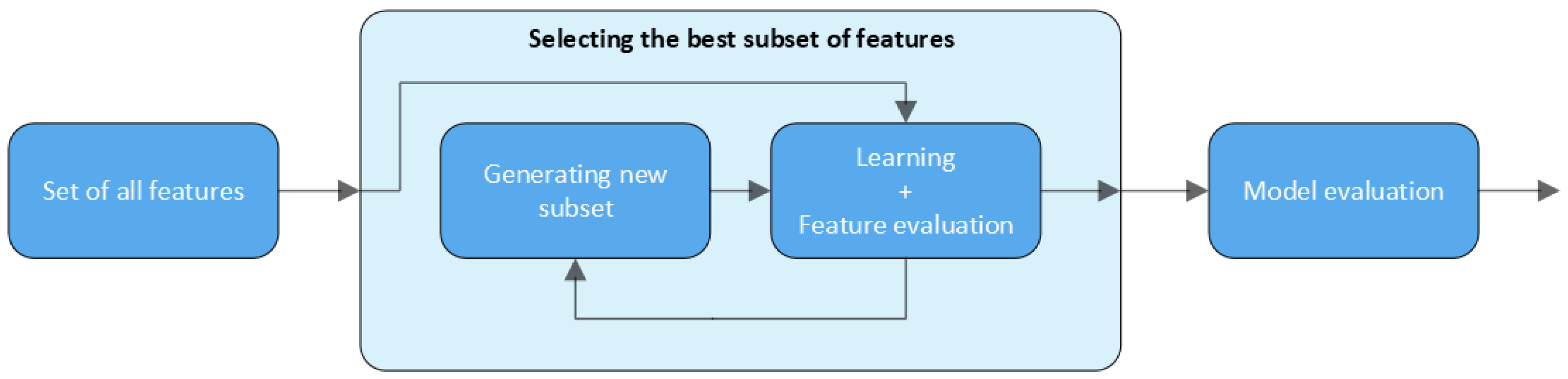
4.2. Wrapper Methods

Wrapper methods select a subset of features using a provided learning algorithm as part of the feature evaluation process, as seen in Figure 2. The learning algorithm serves the purpose of a guide in the search for a better subset. The evaluation function for each possible feature subset returns an estimate of the quality of the model, which therefore causes a better estimate of the algorithm performance. Wrapper methods tend to be slower and exhibit higher computational requirements compared to other methods. Furthermore, they are prone to overfitting, since they rely on a provided classifier. Wrappers have proven to be an interesting choice in many domains for tasks such as DNA analysis, intrusion detection, text categorisation, or information retrieval [56].

Recursive Feature Elimination

Recursive feature elimination (RFE) is a feature selection technique that aims to identify the most relevant features by iteratively considering subsets of features based on their assigned weights by an external estimator. Initially, the estimator is trained on the full feature set and the importance of each feature is evaluated. The features with the lowest importance scores are then eliminated from the current set. RFE provides a systematic approach to progressively narrow down the feature space, focusing on the most influential variables. The combined use of RFE with cross-validation looping can be used to find the optimal number of features [57].

4.3. Embedded Methods

In contrast to the filter and wrapper methods, in embedded methods, the feature selection part and the learning part are performed together, as shown in Figure 3. This method is less computationally expensive than the wrapper method and less prone to overfitting, but unlike the filter method, it can detect feature interactions.

5. Data Preparation and Overview

The following section describes data cleaning and preparation steps performed after initial data analysis. For the research purpose, the CSE CIC IDS2018 dataset [2] was divided into two subsets, hereafter referred to as dataset A and dataset B. The split was determined based on the number of features in the files forming the entire dataset. Dataset A has 80 features and 8,284,181 samples (files: Thursday-15-02-2018, Friday-16-02-2018_clean, Wednesday-21-02-2018, Friday-23-02-2018, Wednesday-28-02-2018, Wednesday-14-02-2018, Thursday-22-02-2018, Thursday-01-03-2018, and Friday-02-03-2018) and dataset B has 84 features and 7,948,748 samples (file Tuesday-20-02-2018.csv). Each sample describes a single flow and a statistic associated with it. Features of the samples along with information on the data types are described in Appendix A.

Overall, the original dataset is nearly ready to work with after being downloaded. There is one minor issue regarding duplicated headers in some files, as mentioned before in some publications. For the sake of subsequent works, the following list presents the files and duplicated headers count: Friday-16-02-2018: 1 duplicate; Thursday-01-03-2018: 25 duplicates; Wednesday-28-02-2018: 33 duplicates. Duplicates were removed.

As mentioned before, dataset A is composed of 80 features collected over a period of 9 days. Nearly 74% of the data is labelled as benign traffic. The remaining part of the data represents groups of some of the most common threats on the internet. The distribution of the labelled data is presented in

Table 2. Overview of types of traffic in dataset A, including the percentage share in the total traffic.

Label	Count	As a Percentage
Benign	6,112,137	73.7808%
DDOS attack-HOIC	686,012	8.2810%
DoS attacks-Hulk	461,912	5.5758%
Bot	286,191	3.4547%
FTP-BruteForce	193,360	2.3341%
SSH-Bruteforce	187,589	2.2644%
Infilteration	161,934	1.9547%
DoS attacks-SlowHTTPTest	139,890	1.6886%
DoS attacks-GoldenEye	41,508	0.5011%
DoS attacks-Slowloris	10,990	0.1327%
DDOS attack-LOIC-UDP	1730	0.0209%
Brute Force-Web	611	0.0074%
Brute Force-XSS	230	0.0028%
SQL Injection	87	0.0011%

.

The cleaning process of dataset A consists of the following actions.

• Removal of the old samples (before year 2000): four entries from Thursday 01-03-2018 and eight entries from Friday 02-03-2018.
• Removal of void features (zeroed columns): Bwd PSH Flags, Bwd URG Flags, Fwd Byts/b Avg, Fwd Pkts/b Avg, Fwd Blk Rate Avg, Bwd Byts/b Avg, Bwd Pkts/b Avg, and Bwd Blk Rate Avg.
• Removal of 22,954 samples with NaN values and replacement of infinity values for 120,000,000 value, as the observed maximum of other features.

Dataset B is composed of 84 features collected over a period of one day. Labelled data are split into two categories, benign and DDoS attacks, in a nearly 93 to 7 ratio. The distribution of the labelled data is presented in

Table 3. Overview of types of traffic in dataset B including the percentage share in the total traffic.

Label	Count	As a Percentage
Benign	7,372,557	92.75%
DDoS attacks-LOIC-HTTP	576,191	7.25%

.

The cleaning process of dataset B consists of the following actions.

• Removal of void features (zeroed columns): Bwd PSH Flags, Fwd URG Flags, Bwd URG Flags, CWE Flag Count, Fwd Byts/b Avg, Fwd Pkts/b Avg, Fwd Blk Rate Avg, Bwd Byts/b Avg, Bwd Pkts/b Avg, and Bwd Blk Rate Avg.
• Remove of non-relevant feature: Flow Id.
• Removal of 36,767 samples with NaN values and replacement of infinity values for 120,000,000 value, as observed maximum of other features.

6. Methodology

The following section describes the methodology behind the conducted experiments. Most parts of the work were performed using a combination of Google Colaboratory, Python 3, and libraries such as pandas, numpy, and sklearn.

6.1. Feature Selection

The original CSE-CIC-IDS2018 dataset has a class imbalance, with roughly 17% of the instances comprising attack (anomalous) traffic, which had to be addressed. The dataset was prepared from a large network of simulated clients and attacking machines, resulting in a dataset that contains 16,233,002 instances gathered from 10 days of network traffic, where each instance represents a single flow and its statistics. After preliminary cleaning and dividing into two sets, we were left with two matrices with around 8 million samples each. For further analysis, the two datasets needed to be additionally processed, ultimately reducing each sample to a reasonable size. As a reasonable parameter for the number of features, a value of 20 was chosen, as most of the conducted experiments in this dataset choose something around this number of features for analysis [22]. Due to insufficient resources, the feature selection process was conducted several times using undersampled datasets. One-tenth of the data from the prepared datasets was used, precisely every tenth sample, sorted by the timestamp set. An overview of the selected parameters for different feature selection methods is shown in

Table 4. Selected parameters for feature selection methods.

Feature Selection Method	Parameters
Random selection	None
Recursive feature elimination with random forest (RFE RF)	Number of trees: 50
Chi2	None
ANOVA F-value	None
Random forest (RF)	Number of trees: 100
Logistic regression with L1 regularisation (LR L1)	Penalty: L1 Solver: saga Dual formulation: false C: 0.1 Class weight: balanced Max number of iterations: 100
Linear support vector classification (LSVC)	Penalty: L1 Dual formulation: false C: 0.01 Class weight: balanced

.

Table 5. Dataset A features ranked by recursive feature elimination with random forest as a classifier.

Feature	Rank	Feature	Rank	Feature	Rank
Dst Port	1	Tot Bwd Pkts	6	ECE Flag Cnt	30
Fwd Seg Size Min	1	Pkt Len Max	7	Bwd IAT Tot	31
Init Fwd Win Byts	1	Subflow Bwd Byts	8	Bwd IAT Max	32
Pkt Size Avg	1	Bwd Pkt Len Std	9	Idle Min	33
Pkt Len Mean	1	TotLen Bwd Pkts	10	Bwd IAT Std	34
Bwd Pkts/s	1	Tot Fwd Pkts	11	Idle Mean	35
Fwd Pkts/s	1	Pkt Len Std	12	Idle Max	36
Fwd Header Len	1	Fwd Seg Size Avg	13	Down/Up Ratio	37
Fwd IAT Min	1	Bwd Pkt Len Mean	14	Active Mean	38
Fwd IAT Max	1	ACK Flag Cnt	15	Idle Std	39
Fwd IAT Mean	1	Flow IAT Std	16	Fwd Pkt Len Min	40
Fwd IAT Tot	1	Subflow Fwd Pkts	17	Active Min	41
Flow IAT Min	1	Bwd Seg Size Avg	18	Active Max	42
Flow IAT Max	1	PSH Flag Cnt	19	Bwd Pkt Len Min	43
Flow IAT Mean	1	Bwd Pkt Len Max	20	Active Std	44
Flow Pkts/s	1	Subflow Fwd Byts	21	Pkt Len Min	45
Bwd Header Len	1	URG Flag Cnt	22	FIN Flag Cnt	46
Flow Byts/s	1	RST Flag Cnt	23	Protocol	47
TotLen Fwd Pkts	1	Fwd Act Data Pkts	24	Fwd PSH Flags	48
Flow Duration	1	Fwd IAT Std	25	SYN Flag Cnt	49
Fwd Pkt Len Max	2	Bwd IAT Min	26	Fwd URG Flags	50
Init Bwd Win Byts	3	Pkt Len Var	27	CWE Flag Count	51
Fwd Pkt Len Mean	4	Bwd IAT Mean	28
Subflow Bwd Pkts	5	Fwd Pkt Len Std	29

and

Table 6. Dataset B features ranked by recursive feature elimination with random forest as a classifier. Features marked in bold were selected for further experiments. The two features marked in bold and italics are used interchangeably with source and destination IP addresses.

Feature	Rank	Feature	Rank Feature	Rank
Src Port	1	Subflow Fwd Pkts	7	Fwd Act Data Pkts	30
Flow IAT Min	1	ACK Flag Cnt	8	Bwd Pkts/s	31
Subflow Fwd Byts	1	Fwd Seg Size Min	9	TotLen Bwd Pkts	32
Fwd IAT Tot	1	Pkt Len Var	10	Protocol	33
Fwd IAT Mean	1	Idle Mean	11	Bwd IAT Tot	34
Fwd Pkt Len Std	1	Tot Fwd Pkts	12	URG Flag Cnt	35
Fwd Pkt Len Mean	1	Fwd Header Len	13	Bwd IAT Mean	36
Fwd IAT Std	1	Bwd Pkt Len Max	14	Bwd Seg Size Avg	37
Fwd Pkt Len Max	1	Idle Max	15	PSH Flag Cnt	38
Fwd IAT Max	1	Subflow Bwd Pkts	16	Pkt Len Min	39
TotLen Fwd Pkts	1	Pkt Len Max	17	Active Max	40
Fwd IAT Min	1	Tot Bwd Pkts	18	Bwd IAT Min	41
Fwd Seg Size Avg	1	Bwd Header Len	19	RST Flag Cnt	42
Flow Duration	1	Idle Min	20	Idle Std	43
Fwd Pkts/s	1	Active Min	21	Bwd IAT Max	44
Dst Port	1	Pkt Size Avg	22	Fwd Pkt Len Min	45
Flow IAT Max	1	Bwd IAT Std	23	ECE Flag Cnt	46
Flow IAT Mean	1	Active Mean	24	Down/Up Ratio	47
Flow Pkts/s	2	Pkt Len Mean	25	SYN Flag Cnt	48
Bwd Pkt Len Std	3	Subflow Bwd Byts	26	Fwd PSH Flags	49
Pkt Len Std	4	Bwd Pkt Len Mean	27	FIN Flag Cnt	50
Flow IAT Std	5	Flow Byts/s	28	Bwd Pkt Len Min	51
Init Fwd Win Byts	6	Init Bwd Win Byts	29	Active Std	52

present ranked lists of features selected, respectively, from datasets A and B by RFE RF. Among all the methods, this one most accurately captures the dynamics of the datasets. As demonstrated in [58], information about inter-arrival times (IATs) may prove their potential to provide a valuable contribution to network analysis. Figure 4 and Figure 5 provide an overview of the selected features by method, and

Table 7. Comparison of selected features by method using Jaccard similarity coefficient for dataset A.

Method	Random	RFE RF	Chi2	ANOVA F-Value	RF	LR l1	LSVC
Random	100.00%	11.11%	8.11%	11.11%	11.11%	14.29%	8.11%
RFE RF	11.11%	100.00%	33.33%	25.00%	90.48%	14.29%	5.26%
Chi2	8.11%	33.33%	100.00%	14.29%	29.03%	0.00%	2.56%
ANOVA F-value	11.11%	25.00%	14.29%	100.00%	25.00%	29.03%	25.00%
RF	11.11%	90.48%	29.03%	25.00%	100.00%	14.29%	5.26%
LR L1	14.29%	14.29%	0.00%	29.03%	14.29%	100.00%	25.00%
LSVC	8.11%	5.26%	2.56%	25.00%	5.26%	25.00%	100.00%

and

Table 8. Comparison of selected features by method using Jaccard similarity coefficient for dataset B.

Method	Random	RFE RF	Chi2	ANOVA F-Value	RF	LR l1	LSVC
Random	100.00%	11.11%	17.65%	14.29%	5.26%	14.29%	17.65%
RFE RF	11.11%	100.00%	29.03%	37.93%	81.82%	25.00%	14.29%
Chi2	17.65%	29.03%	100.00%	11.11%	25.00%	14.29%	0.00%
ANOVA F-value	14.29%	37.93%	11.11%	100.00%	37.93%	21.21%	29.03%
RF	5.26%	81.82%	25.00%	37.93%	100.00%	29.03%	14.29%
LR L1	14.29%	25.00%	14.29%	21.21%	29.03%	100.00%	17.65%
LSVC	17.65%	14.29%	0.00%	29.03%	14.29%	17.65%	100.00%

represent the degree of similarity in feature selection using the Jaccard similarity coefficient. Finally,

Table 9. Comparison of selected features by method using Jaccard similarity coefficient for datasets A and B.

Method	Random	A RFE RF	A Chi2	A ANOVA F-Value	A RF	A LR l1	A LSVC
Random	100.00%	11.11%	8.11%	11.11%	11.11%	14.29%	8.11%
B RFE RF	11.11%	42.86%	33.33%	21.21%	42.86%	14.29%	0.00%
B Chi2	17.65%	29.03%	60.00%	5.26%	29.03%	2.56%	0.00%
B ANOVA F-value	14.29%	17.65%	11.11%	17.65%	21.21%	33.33%	17.65%
B RF	5.26%	42.86%	37.93%	25.00%	42.86%	17.65%	0.00%
B LR L1	14.29%	5.26%	14.29%	14.29%	8.11%	25.00%	2.56%
B LSVC	17.65%	25.00%	2.56%	42.86%	29.03%	37.93%	25.00%

provides a comparison of selected features between all selected feature sets for both datasets. It can be observed that there are no major similarities between the sets of selected attributes, which confirms that there is no single predefined answer when selecting features. Interestingly, the features selected just partly match those proposed by the authors of the CICIDS2018 dataset [59].

6.2. Models and Training

Prepared datasets were split into training and test stratified subsets in an 80:20 ratio using the train_test_split function from the sklearn library. Subsequent experiments were performed using the stratified 10-fold cross-validation technique. RF, MLP, and LSVC were selected in order to evaluate the impact of the earlier efforts. These algorithms effectively capture the diverse problem-solving groups of strategies and represent some of the most commonly used approaches in this area. Each test’s pipeline consists of a pipeline with one of the selected models and a scaler at the input. Except for the MLP model, where MinMaxScaler was used instead of StandardScaler. Due to insufficient resources, the LSVC model was not used for dataset A. The configuration of all the models used is given in

Table 10. The configuration of all the models used in experiments with dataset A.

Model	Configuration
Dummy classifier	Strategy = ‘most_frequent’
Random forest classifier (RF) from sklearn.ensemble package	n_estimators = 12 criterion = ‘gini’ max_depth = 22 min_samples_split = 10 class_weight = ‘balanced’
Multi-layer perceptron classifier (MLP) from sklearn.neural_network package	hidden_layer_sizes = (15) activation = ‘relu’ solver = ‘adam’ batch_size = ‘auto’ alpha = 0.001 learning_rate_init = 0.001 max_iter = 20

and

Table 11. The configuration of all the models used in experiments with dataset B.

Model	Configuration
Dummy classifier	strategy = ‘most_frequent’
Random forest classifier (RF) from sklearn.ensemble package	n_estimators = 12 criterion = ‘gini’ max_depth = 22 min_samples_split = 10 random_state = 2021 class_weight = ‘balanced’
Multi-layer perceptron classifier (MLP) from sklearn.neural_network package	hidden_layer_sizes = (15) activation = ‘relu’ solver = ‘adam’ batch_size = ‘auto’ alpha = 0.001 learning_rate_init = 0.001 max_iter = 20
Linear support vector classifier (LSVC) from sklearn.svm package	penalty = ‘l2’ loss = ‘squared_hinge’ dual = False C = 1.0 class_weight = ‘balanced’ max_iter = 50

.

7. Results

Given the results, there is a clear difference between cases of datasets A and B, with the first one representing multiclass classification problems (14 classes), and the second one representing binary classification (benign and DDoS). In both cases, we can see the slight advantage of the three-layer MLP model over RF, which prevails in publications related to network threat detection. The linear support vector classifier achieved reasonable results. Considering the full results (Figure 6, Figure 7, Figure 8, Figure 9 and Figure 10), we can confirm the statement given in [57], suggesting that the efficiency of feature selection using random forest is better than that based on the support vector classifier. Interestingly, LSVC-based feature selection performed better with the task of binary classification. In the case of multiclass, the basic solution with randomly selected features performs better. For the case of both subsets, the effectiveness of the chi-square method is not satisfying, although better results can be observed for the binary classification task in combination with RF and MLP models.

As mention in the previous section, configurations of the RF and RFE RF methods differs slightly. Overall, RF, with double the number of trees compared to RFE RF, shows a slight advantage. Moreover, when we take into consideration the processing time, the RF-based feature selection should be preferred over the RFE RF method. In accordance with [18], Cohen’s kappa and F1-score metrics proved to be more suitable for comparison with imbalanced datasets compared to the widely used accuracy metric. The results also support the statement in [60] that, although AUC metrics might be useful as summary statistics, there is a lack of visual inspection capability of the curves to provide more information about evaluation.

Taking a holistic view of all the charts we can see how important it is to perform a comprehensive analysis of the subject. Not every feature selection method behaves exactly the same with different classifiers and classification tasks. This is why it is important to pay extra attention to data analysis and comparison of outcomes. Firstly, by taking into account at least two metrics, it is possible to capture the characteristics of the domain under evaluation. Secondly, the inclusion of a baseline model in the results shows the complexity of the problem and provides minimum expectations for the newly developed solution. The same holds true for the basic solution of feature selection (random feature selection). As such, for publications proposing yet another model for threat detection for datasets achieving over 99% effectiveness this may come as a surprise. However, given that some of the data may be filtered for the purposes of that new research and that the basic model can achieve efficiency of over 90% for basic metrics that do not take into account the distribution of the data, these doubts can be alleviated. The model and results are correct, but the context may not be fully covered.

As mentioned earlier, the classification issues differ between subsets. The case for subset A represents a multilabel classification problem while the case for subset B represents a binary classification problem. The former case is, by definition, more difficult, represented by the differences in the results obtained in each metric. What seems interesting is that, using an appropriate feature selection method, the MLP model gives superior results when compared to the RF model, which is often highlighted in the literature.

A comparison between the ANOVA F-value (filter method) and RFE RF (wrapper method) (Figure 11 and Figure 12) shows that, in the case of the CSE CIC IDS2018 dataset, there is no major difference in the observed results. This contrasts to the time aspect of the experiments, where the wrapper method requires much more of this resource. Overall, the best results were achieved with the embedded feature selection method: feature selection based on random forest. In this case, however, a different aspect is noteworthy. Although the feature selection methods do not exhibit significant differences in their outcomes, the performance variations among the models become significantly pronounced. This example underscores the importance of presenting the results alongside the baseline model, as it provides valuable context and perspective. Moreover, including two or three additional metrics does not impose a substantial overhead but greatly enhances the comparability of the proposed solutions for future researchers. This practice not only improves the overall understanding of the findings but also fosters a more comprehensive and meaningful comparison between different approaches. By incorporating these additional metrics, we contribute to the advancement of research in the field and facilitate more informed decision-making in subsequent studies.

Confidence intervals are not shown in the figures because of their minor values. For the sake of transparency, the most significant values for experiments with datasets A and B are presented in Figure 13 and Figure 14, respectively. The rest of the confidence intervals values were below 0.005.

The most challenging part, in addition to data preparation, which took around 60% of the total work time (domain average for this task is around 60–70% of the total work time), was to constantly optimise the use of resources, with an emphasis on RAM usage, due to the large amount of data being processed. The duration of each test cycle, which was counted in days, was also a problem. Due to limited resources and time constraints, we were unable to properly optimise the parameters of every feature selection algorithm for every machine learning model. Additionally, a detailed exploration of the influence of the number of processed features remains an area that requires further investigation in future work. Although these aspects were not comprehensively addressed in our current study, they present valuable directions for future research and development in this field.

8. Conclusions

This paper discusses the problems of feature selection and metric choice for the performance evaluation of network traffic threat detection solutions that use machine learning techniques. These network solutions requires rapidity of response and accuracy as well as precision of detection. Data science tools, including machine learning approaches, have a broad range of applications. As research shows, the ICT domain is also a place where their use delivers promising results. That is mainly because of the nature of this area. By definition, ICT infrastructure including smart grid infrastructure directly or indirectly process a significant volume of data, which is often structured and is appropriate for big data applications. In addition to domain knowledge, a proper understanding of a specific case, the related data, and the understanding and awareness of available tools are also essential. These tools include pre-processing methods, dimension reduction and feature selection techniques, and means of verifying the correct and effective operation of the developed application. The proper adoption of data analysis best practice in research is able to positively affect the quality of research in a given area and the authenticity of the achieved results; however, we noticed that this aspect of research is still frequently overlooked.

In this work, we proposed new feature sets for training machine learning algorithms on the CSE CIC IDS2018 dataset, suggested the effective techniques for features selection, and proposed the appropriate method for comparing results between different studies in the context of imbalanced datasets and threat identification. Dismissing part of the features may appear to be an information loss. However, the use of a streamlined feature set in machine learning can lead to faster, more accurate, and more interpretable models, while also lowering computational complexity and storage requirements. Regarding the comparison of the effectiveness of the proposed ML-based solutions for threat detection, at this moment there is no common framework used whatsoever. Therefore, we suggest several general steps that should be taken into consideration before publishing future findings. To reach these conclusions, firstly, we reviewed the available datasets and papers related to machine learning-based threat detection in the ICT domain. Secondly, we identified the most frequently used algorithms for threat, anomaly, or incident detection. On the basis of this, we identified the most prevalent mistakes and shortcomings associated with machine learning-based solutions in ICT applications. To examine the underlying problems, we used an imbalanced CSE CIC IDS2018 dataset that contains labelled network attacks and appropriately captures the reality of the network environment. Then, we compared the effectiveness of the filter, wrapper, and embedded methods for feature selection, as well as accuracy, F1-score, Cohen’s kappa, and ROC AUC metrics. Subsequent experiments were performed using the stratified 10-fold cross-validation technique, and we used random forest, multi-layer perceptron, linear support vector classifier, and dummy classifier, which serve the purpose of a reference point, in order to evaluate the impact of the earlier efforts with regard to multiclass classification and binary classification problems.

As a short summary of the article and our work, the following conclusions can be presented:

• Feature selection methods based on random forest, ANOVA F-value and logistic regression with L1 regularisation have proven their robustness and are recommended for processing large datasets.
• The baseline model serves superbly as a reference point throughout the research. The same holds true for the basic solution for feature selection, which relied on randomly selected features. This aspect should not be ignored in scientific research, as it appears to be the case in most publications.
• Compared to the widely used accuracy metric, Cohen’s kappa and F1-score metrics are more suitable for comparison with imbalanced datasets. Once again, the use of more than one metric should not be neglected in academic studies, especially in the case of experiments on imbalanced datasets where appropriate metrics need to be used.
• Finally, it is fundamental to have a clear and thorough description of the entire process of model creation, starting from data preparation, through model setup, testing methodology, and result visualisation. The absence of such information undermines the credibility of a study and makes it impossible to make meaningful comparisons with future research.

To conclude, with reference to the data, information, knowledge, wisdom (DIKW) and data science pyramids, what is important in data science research is not only the final result achieved by the model but also the way in which the result was obtained and the model was developed. In order to gain deeper insights and wisdom from the developed model, it is crucial to have a strong foundation at the lower levels of the pyramid, starting with the proper preparation of data and information. The quality of the data and the methods used to process these data are essential to the accuracy and reliability of the final model and its results.

References

1. Ding, J.; Qammar, A.; Zhang, Z.; Karim, A.; Ning, H. Cyber Threats to Smart Grids: Review, Taxonomy, Potential Solutions, and Future Directions. Energies 2022, 15, 6799. [Google Scholar] [CrossRef]
2. Communications Security Establishment and The Canadian Institute for Cybersecurity—A Realistic Cyber Defense Dataset (CSE-CIC-IDS2018). 2018. Available online: https://registry.opendata.aws/cse-cic-ids2018 (accessed on 6 October 2022).
3. Rapacz, S.; Chołda, P.; Natkaniec, M. A Method for Fast Selection of Machine-Learning Classifiers for Spam Filtering. Electronics 2021, 10, 2083. [Google Scholar] [CrossRef]
4. McQuin, C.; Goodman, A.; Chernyshev, V.; Kamentsky, L.; Cimini, B.A.; Karhohs, K.W.; Doan, M.; Ding, L.; Rafelski, S.M.; Thirstrup, D.; et al. CellProfiler 3.0: Next-generation image processing for biology. PLoS Biol. 2018, 16, e2005970. [Google Scholar] [CrossRef] [Green Version]
5. Weiss, J.; Raghu, V.K.; Bontempi, D.; Christiani, D.C.; Mak, R.H.; Lu, M.T.; Aerts, H.J. Deep learning to estimate lung disease mortality from chest radiographs. Nat. Commun. 2023, 14, 2797. [Google Scholar] [CrossRef] [PubMed]
6. Wu, C.; Hong, L.; Wang, L.; Zhang, R.; Pijush, S.; Zhang, W. Prediction of wall deflection induced by braced excavation in spatially variable soils via convolutional neural network. Gondwana Res. 2022. [Google Scholar] [CrossRef]
7. Zhang, W.; Wu, C.; Tang, L.; Gu, X.; Wang, L. Efficient time-variant reliability analysis of Bazimen landslide in the Three Gorges Reservoir Area using XGBoost and LightGBM algorithms. Gondwana Res. 2022. [Google Scholar] [CrossRef]
8. Baryannis, G.; Dani, S.; Antoniou, G. Predicting supply chain risks using machine learning: The trade-off between performance and interpretability. Future Gener. Comput. Syst. 2019, 101, 993–1004. [Google Scholar] [CrossRef]
9. Ni, D.; Xiao, Z.; Lim, M.K. A systematic review of the research trends of machine learning in supply chain management. Int. J. Mach. Learn. Cybern. 2019, 11, 1463–1482. [Google Scholar] [CrossRef]
10. Mololoth, V.K.; Saguna, S.; Åhlund, C. Blockchain and Machine Learning for Future Smart Grids: A Review. Energies 2023, 16, 528. [Google Scholar] [CrossRef]
11. Tufail, S.; Parvez, I.; Batool, S.; Sarwat, A. A Survey on Cybersecurity Challenges, Detection, and Mitigation Techniques for the Smart Grid. Energies 2021, 14, 5894. [Google Scholar] [CrossRef]
12. Kanimozhi, V.; Jacob, T.P. Artificial Intelligence based Network Intrusion Detection with Hyper-Parameter Optimization Tuning on the Realistic Cyber Dataset CSE-CIC-IDS2018 using Cloud Computing. In Proceedings of the 2019 International Conference on Communication and Signal Processing (ICCSP), Melmaruvathur, India, 4–6 April 2019; pp. 33–36. [Google Scholar] [CrossRef]
13. Gardner, M.; Dorling, S. Artificial neural networks (the multilayer perceptron)—A review of applications in the atmospheric sciences. Atmos. Environ. 1998, 32, 2627–2636. [Google Scholar] [CrossRef]
14. Chastikova, V.A.; Sotnikov, V.V. Method of analyzing computer traffic based on recurrent neural networks. J. Phys. Conf. Ser. 2019, 1353, 012133. [Google Scholar] [CrossRef]
15. Hochreiter, S.; Schmidhuber, J. Long Short-Term Memory. Neural Comput. 1997, 9, 1735–1780. [Google Scholar] [CrossRef] [PubMed]
16. Lin, T.Y.; Goyal, P.; Girshick, R.; He, K.; Dollár, P. Focal Loss for Dense Object Detection. IEEE Trans. Pattern Anal. Mach. Intell. 2020, 42, 318–327. [Google Scholar] [CrossRef] [Green Version]
17. Gu, Q.; Zhu, L.; Cai, Z. Evaluation Measures of the Classification Performance of Imbalanced Data Sets. In Proceedings of the Computational Intelligence and Intelligent Systems; Cai, Z., Li, Z., Kang, Z., Liu, Y., Eds.; Springer: Berlin/Heidelberg, Germany, 2009; pp. 461–471. [Google Scholar]
18. Fatourechi, M.; Ward, R.K.; Mason, S.G.; Huggins, J.; Schlögl, A.; Birch, G.E. Comparison of Evaluation Metrics in Classification Applications with Imbalanced Datasets. In Proceedings of the 2008 Seventh International Conference on Machine Learning and Applications, San Diego, CA, USA, 11–13 December 2008; pp. 777–782. [Google Scholar] [CrossRef]
19. Chadza, T.; Kyriakopoulos, K.G.; Lambotharan, S. Contemporary Sequential Network Attacks Prediction using Hidden Markov Model. In Proceedings of the 2019 17th International Conference on Privacy, Security and Trust (PST), Fredericton, NB, Canada, 26–28 August 2019; pp. 1–3. [Google Scholar] [CrossRef] [Green Version]
20. Weng, C.G.; Poon, J. A New Evaluation Measure for Imbalanced Datasets. In Proceedings of the 7th Australasian Data Mining Conference, Glenelg/Adelaide, SA, Australia, 27–28 November 2008; Volume 87, pp. 27–32. [Google Scholar]
21. Bekkar, M.; Djema, H.; Alitouche, T. Evaluation measures for models assessment over imbalanced data sets. J. Inf. Eng. Appl. 2013, 3, 27–38. [Google Scholar]
22. Filho, F.; Silveira, F.; Junior, A.; vargas solar, G.; Silveira, L. Smart Detection: An Online Approach for DoS/DDoS Attack Detection Using Machine Learning. Secur. Commun. Netw. 2019, 2019, 749. [Google Scholar] [CrossRef]
23. Breiman, L. Random Forests. Mach. Learn. 2001, 45, 5–32. [Google Scholar] [CrossRef] [Green Version]
24. Safavian, S.; Landgrebe, D. A survey of decision tree classifier methodology. IEEE Trans. Syst. Man Cybern. 1991, 21, 660–674. [Google Scholar] [CrossRef] [Green Version]
25. Dreiseitl, S.; Ohno-Machado, L. Logistic regression and artificial neural network classification models: A methodology review. J. Biomed. Inform. 2002, 35, 352–359. [Google Scholar] [CrossRef] [Green Version]
26. Bottou, L. Large-Scale Machine Learning with Stochastic Gradient Descent. In Proceedings of the COMPSTAT’2010; Lechevallier, Y., Saporta, G., Eds.; Springer: Heidelberg, Germany, 2010; pp. 177–186. [Google Scholar]
27. Hu, W.; Hu, W.; Maybank, S. AdaBoost-Based Algorithm for Network Intrusion Detection. IEEE Trans. Syst. Man Cybern. Part B (Cybernetics) 2008, 38, 577–583. [Google Scholar] [CrossRef] [PubMed]
28. Raeder, T.; Forman, G.; Chawla, N.V. Learning from Imbalanced Data: Evaluation Matters. In Data Mining: Foundations and Intelligent Paradigms: Volume 1: Clustering, Association and Classification; Holmes, D.E., Jain, L.C., Eds.; Springer: Berlin/Heidelberg, Germany, 2012; pp. 315–331. [Google Scholar] [CrossRef]
29. Basnet, R.B.; Shash, R.; Johnson, C.; Walgren, L.; Doleck, T. Towards Detecting and Classifying Network Intrusion Traffic Using Deep Learning Frameworks. J. Internet Serv. Inf. Secur. 2019, 9, 1–17. [Google Scholar]
30. Ferrag, M.A.; Maglaras, L.; Moschoyiannis, S.; Janicke, H. Deep learning for cyber security intrusion detection: Approaches, datasets, and comparative study. J. Inf. Secur. Appl. 2020, 50, 102419. [Google Scholar] [CrossRef]
31. Vinayakumar, R.; Soman, K.; Poornachandran, P. Evaluation of Recurrent Neural Network and Its Variants for Intrusion Detection System IDS. Int. J. Inf. Syst. Model. Des. 2017, 8, 43–63. [Google Scholar] [CrossRef]
32. Al-Mhiqani, M.; Ahmad, R.; Zainal Abidin, Z. An Integrated Imbalanced Learning and Deep Neural Network Model for Insider Threat Detection. Int. J. Adv. Comput. Sci. Appl. 2021, 12, 2021. [Google Scholar] [CrossRef]
33. Chen, H.; Murray, A. Continuous restricted Boltzmann machine with an implementable training algorithm. Vision Image Signal Process. IEE Proc. 2003, 150, 153–158. [Google Scholar] [CrossRef] [Green Version]
34. Gao, N.; Gao, L.; Gao, Q.; Wang, H. An Intrusion Detection Model Based on Deep Belief Networks. In Proceedings of the 2014 Second International Conference on Advanced Cloud and Big Data, Huangshan, China, 20–22 November 2014; pp. 247–252. [Google Scholar] [CrossRef]
35. Alom, M.Z.; Bontupalli, V.; Taha, T.M. Intrusion detection using deep belief networks. In Proceedings of the 2015 National Aerospace and Electronics Conference (NAECON), Dayton, OI, USA, 15–19 June 2015; pp. 339–344. [Google Scholar] [CrossRef]
36. Li, Y. Research on Application of Convolutional Neural Network in Intrusion Detection. In Proceedings of the 2020 7th International Forum on Electrical Engineering and Automation (IFEEA), Hefei, China, 25–27 September 2020; pp. 720–723. [Google Scholar] [CrossRef]
37. Salakhutdinov, R.; Hinton, G. Deep Boltzmann Machines. In Proceedings of the Twelth International Conference on Artificial Intelligence and Statistics, Clearwater Beach, FL, USA, 16–18 April 2009; van Dyk, D., Welling, M., Eds.; Hilton Clearwater Beach Resort: Clearwater Beach, FL, USA, 2009; Volume 5, pp. 448–455. [Google Scholar]
38. Seo, S.; Park, S.; Kim, J. Improvement of Network Intrusion Detection Accuracy by Using Restricted Boltzmann Machine. In Proceedings of the 2016 8th International Conference on Computational Intelligence and Communication Networks (CICN), Dehradun, India, 23–25 December 2016; pp. 413–417. [Google Scholar] [CrossRef]
39. Chuang, P.J.; Wu, D.Y. Applying Deep Learning to Balancing Network Intrusion Detection Datasets. In Proceedings of the 2019 IEEE 11th International Conference on Advanced Infocomm Technology (ICAIT), Jinan, China, 18–20 October 2019; pp. 213–217. [Google Scholar] [CrossRef]
40. Xu, C.; Shen, J.; Du, X.; Zhang, F. An Intrusion Detection System Using a Deep Neural Network With Gated Recurrent Units. IEEE Access 2018, 6, 48697–48707. [Google Scholar] [CrossRef]
41. Atefinia, R.; Ahmadi, M. Network Intrusion Detection using Multi-Architectural Modular Deep Neural Network. J. Supercomput. 2021, 77, 3571–3593. [Google Scholar] [CrossRef]
42. Karatas, G.; Demir, O.; Sahingoz, O.K. Increasing the Performance of Machine Learning-Based IDSs on an Imbalanced and Up-to-Date Dataset. IEEE Access 2020, 8, 32150–32162. [Google Scholar] [CrossRef]
43. Chawla, N.V.; Bowyer, K.W.; Hall, L.O.; Kegelmeyer, W.P. SMOTE: Synthetic Minority over-Sampling Technique. J. Artif. Int. Res. 2002, 16, 321–357. [Google Scholar] [CrossRef]
44. Sawadogo, L.M.; Bassolé, D.; Koala, G.; Sié, O. Intrusions Detection and Classification Using Deep Learning Approach. In Proceedings of the Research in Computer Science and Its Applications, Virtual, 17–19 June 2021; Faye, Y., Gueye, A., Gueye, B., Diongue, D., Nguer, E.H.M., Ba, M., Eds.; Springer: Cham, Switzerland, 2021; pp. 40–51. [Google Scholar]
45. Stryczek, S.; Natkaniec, M. Internet Threat Detection in Smart Grids Based on Network Traffic Analysis Using LSTM, IF, and SVM. Energies 2023, 16, 329. [Google Scholar] [CrossRef]
46. Peng, C.; Sun, H.; Yang, M.; Wang, Y.L. A Survey on Security Communication and Control for Smart Grids Under Malicious Cyber Attacks. IEEE Trans. Syst. Man Cybern. Syst. 2019, 49, 1554–1569. [Google Scholar] [CrossRef]
47. Gunduz, M.Z.; Das, R. Cyber-security on smart grid: Threats and potential solutions. Comput. Netw. 2020, 169, 107094. [Google Scholar] [CrossRef]
48. Sakhnini, J.; Karimipour, H.; Dehghantanha, A.; Parizi, R.M.; Srivastava, G. Security aspects of Internet of Things aided smart grids: A bibliometric survey. Internet Things 2021, 14, 100111. [Google Scholar] [CrossRef]
49. Caprolu, M.; Raponi, S.; Di Pietro, R.; Antonopoulos, A. FORTRESS: An Efficient and Distributed Firewall for Stateful Data Plane SDN. Sec. Commun. Netw. 2019, 2019, 6874592. [Google Scholar] [CrossRef] [Green Version]
50. Weber, R.; Schek, H.J.; Blott, S. A Quantitative Analysis and Performance Study for Similarity-Search Methods in High-Dimensional Spaces. In Proceedings of the 24rd International Conference on Very Large Data Bases, San Francisco, CA, USA, 26–29 August 1998; VLDB ’98. pp. 194–205. [Google Scholar]
51. Butcher, B.; Smith, B.J. Feature Engineering and Selection: A Practical Approach for Predictive Models. Am. Stat. 2020, 74, 308–309. [Google Scholar] [CrossRef]
52. Borisov, V.; Haug, J.; Kasneci, G. CancelOut: A Layer for Feature Selection in Deep Neural Networks. In Proceedings of the Artificial Neural Networks and Machine Learning—ICANN 2019: Deep Learning, Munich, Germany, 17–19 September 2019; Tetko, I.V., Kůrková, V., Karpov, P., Theis, F., Eds.; Springer: Cham, Switzerland, 2019; pp. 72–83. [Google Scholar]
53. Gidey, H.T.; Guo, X.; Li, L.; Zhang, Y. Heterogeneous Transfer Learning for Wi-Fi Indoor Positioning Based Hybrid Feature Selection. Sensors 2022, 22, 5840. [Google Scholar] [CrossRef] [PubMed]
54. Attallah, O. Tomato Leaf Disease Classification via Compact Convolutional Neural Networks with Transfer Learning and Feature Selection. Horticulturae 2023, 9, 149. [Google Scholar] [CrossRef]
55. Hall, M.A. Correlation-Based Feature Selection for Machine Learning. Ph.D. Thesis, The University of Waikato, Hamilton, New Zealand, 1999. [Google Scholar]
56. Bolón-Canedo, V.; Sánchez-Maroño, N.; Alonso-Betanzos, A. A review of feature selection methods on synthetic data. Knowl. Inf. Syst. 2013, 34, 483–519. [Google Scholar] [CrossRef]
57. Granitto, P.M.; Furlanello, C.; Biasioli, F.; Gasperi, F. Recursive feature elimination with random forest for PTR-MS analysis of agroindustrial products. Chemom. Intell. Lab. Syst. 2006, 83, 83–90. [Google Scholar] [CrossRef]
58. Zimmermann, J.; Clark, A.; Mohay, G.; Pouget, F.; Dacier, M. The use of packet inter-arrival times for investigating unsolicited Internet traffic. In Proceedings of the First International Workshop on Systematic Approaches to Digital Forensic Engineering (SADFE’05), Taiwan, China, 7–9 November 2005; pp. 89–104. [Google Scholar] [CrossRef] [Green Version]
59. Sharafaldin, I.; Habibi Lashkari, A.; Ghorbani, A. Toward Generating a New Intrusion Detection Dataset and Intrusion Traffic Characterization. In Proceedings of the 4th International Conference on Information Systems Security and Privacy, Madeira, Portugal, 22–24 January 2018; pp. 108–116. [Google Scholar] [CrossRef]
60. Fernández, A.; García, S.; Galar, M.; Prati, R.C.; Krawczyk, B.; Herrera, F. Learning from Imbalanced Data Sets; Springer: Cham, Switzerland, 2018. [Google Scholar] [CrossRef]
Figure 1. General scheme of a filter method for feature selection.
Energies 16 04632 g001
Figure 2. General scheme of a wrapper method for feature selection.
Energies 16 04632 g002
Figure 3. General scheme of an embedded method for feature selection.
Energies 16 04632 g003
Figure 4. Summary of selected features by different methods for dataset A.
Energies 16 04632 g004
Figure 5. Summary of selected features by different methods for dataset B.
Energies 16 04632 g005
Figure 6. Comparison of the influence of feature selection methods on the effectiveness of the random forest model with dataset A.
Energies 16 04632 g006
Figure 7. Comparison of the influence of feature selection methods on the effectiveness of the multi-layer perceptron model with dataset A.
Energies 16 04632 g007
Figure 8. Comparison of the influence of feature selection methods on the effectiveness of the random forest model with dataset B.
Energies 16 04632 g008
Figure 9. Comparison of the influence of feature selection methods on the effectiveness of the multi-layer perceptron model with dataset B.
Energies 16 04632 g009
Figure 10. Comparison of the influence of feature selection methods on the effectiveness of the linear support vector classifier model with dataset B.
Energies 16 04632 g010
Figure 11. Comparison between filter (ANOVA F-value) and wrapper (RFE with RF) feature selection methods with dataset A. Each row represents a different type of metric.
Energies 16 04632 g011
Figure 12. Comparison between filter (ANOVA F-value) and wrapper (RFE with RF) feature selection methods with dataset B. Each row represents a different type of metric.
Energies 16 04632 g012
Figure 13. Top 95 confidence intervals for results of experiments with dataset A. X-axis is represented by the type of a model, a feature set, and a metric from the bottom to the top.
Energies 16 04632 g013
Figure 14. Top 95 confidence intervals for results of experiments with dataset B. X-axis is represented by the type of a model, a feature set, and a metric from the bottom to the top.
Energies 16 04632 g014