1. Introduction
Notice: This manuscript has been authored by UT-Battelle, LLC, under contract DE-AC05-00OR22725 with the US Department of Energy (DOE). The US government retains and the publisher, by accepting the article for publication, acknowledges that the US government retains a nonexclusive, paid-up, irrevocable, worldwide license to publish or reproduce the published form of this manuscript, or allow others to do so, for US government purposes. DOE will provide public access to these results of federally sponsored research in accordance with the DOE Public Access Plan (
http://energy.gov/downloads/doe-public-access-plan, accessed on 10 May 2023).
1.1. Background
Buildings are responsible for about 40% of the total energy consumed in the United States [
1], accounting for 75% of the total electricity consumption and 78% of the 2:00–8:00 p.m. peak period of electricity use [
2,
3]. As of 2020, 75% of the homes in the United States use central air conditioning [
4]. Since space conditioning loads comprise about half of the total building’s load [
2], residential buildings present an opportunity to reduce peak energy demands by managing a building’s heating and cooling demand and can relieve stress on the electric grid during peak times by shifting the peak loads [
5,
6,
7,
8].
Thermal energy storage (TES) has been identified as a key enabler for reducing peak demand and providing resilience for reliable operation during power outages, as described in the US Department of Energy’s Grid-interactive Efficient Buildings report [
2]. According to the report [
2], consumers who pay demand charges or time-of-use (TOU) rates are generally the most financially driven to adopt the technology because TES is beneficial for shifting predictable daily loads for demand response.
The US Census Bureau reports that more than 44% of US houses were built before 1970 and were constructed according to outdated standards [
9]. As a result, oversized heat pumps (HPs) are essential for regulating humidity and temperature inside the house. Although renovating the house or fully upgrading the conventional heating, ventilation, and air conditioning (HVAC) equipment can be costly, heat pump (HP) systems are adaptable because they are able to respond smartly to the fluctuations in peak demand. The capabilities of HPs and TES can be combined by integrating these technologies. This integration allows the use of already-established technology and resources with minimal equipment to reduce the installation complexity and TES footprint [
2,
10].
Many possibilities exist for packaging phase change material (PCM)-TES in various configurations. Passive TES configurations are the most common in the literature, whereby TES charging and discharging occur according to one or more uncontrolled independent variables such as ambient temperature and PCM melting temperature. Passive TES may provide energy and cost saving benefits, but they pose challenges such as complex installation, material encapsulation, space constraints, and additional controls and components. Furthermore, passive TES are not ideal for peak demand reduction because they do not have control over TES operation [
11,
12,
13,
14,
15,
16]. In active TES configurations, the decision of when to charge and discharge is determined by controller hardware. The major benefit of active TES configurations is the flexibility allowing them to be installed in an existing building infrastructure without needing a significant construction—the TES may be separate and removed from the space and simply integrated into existing HP equipment. The heat transfer is mediated by the HP in active HP–integrated TES (HP-TES) configurations, and the user can control the charging and discharging process based on cooling or heating demand because HP-TES is programable with the thermostat [
10].
1.2. State of the Art
Researchers have installed PCM via passive TES configurations in walls, ceilings, windows, or embedded directly into building materials such as concrete [
17,
18,
19,
20,
21,
22]. HP-integrated active TES—where TES has been coupled to or installed in HP components such as an evaporator or condenser [
23,
24,
25,
26,
27,
28]—is the focus of this paper. The techno-economic value for each configuration varies by charging and discharging operation, storage capacity and the material used. A previous review [
10] pointed out that researchers have shown energy savings of 9–62% when using TES, but the PCM temperature and storage varies in each study [
10].
A particularly promising active HP-TES configuration by Dong et al. [
23] offers large performance improvement with minimum modification while reducing the TES footprint. The ice-based TES system simulated for 100 residential buildings in Tennessee was mediated by HP and absorbs the air conditioner’s condenser heat during peak hours. Peak load of 12.7% was shifted, saving 19% of winter electricity cost and 13% of electric consumption for space heating on a winter day in Nashville.
The selection of PCM, phase change temperature (PCT) and storage capacity are important to design the appropriate TES [
29]. Various approaches that choose the PCT can be found in the literature to maximize their performance for space conditioning in buildings. Waqas et al. [
29] argued that PCM temperature selection should be close to the comfort temperature of the chosen climate location. Medved and Arkar [
30] studied passive cooling for continental climates and found the PCM with a melting point equal to the average temperature of the hottest month was the most appropriate choice (i.e., 20–22 °C). Waqas and Kumar [
31] demonstrated optimum PCM storage unit performance by selecting a PCM with the melting point equal to the comfort temperature of the hottest month for free cooling.
A single PCM unit for heating and cooling was analyzed for the subtropical humid climate of Islamabad, Pakistan, which experiences large variations in summer and winter temperatures [
32]. A commercial PCM (salt and paraffin blend) was used, and a parametric study was performed. The optimum melting point was approximately 29 °C for summer and approximately 21 °C for winter. Both seasons could have optimized performance at approximately 27.5 °C, but the cooling capacity dropped drastically below this point. The study concluded that to choose a single melting temperature for both applications, the PCM melting point that maximized summer cooling could be used for winter heating but not vice versa [
32].
Passive PCM-TES is proven in the literature to be effective for space cooling, but for the climates with less significant diurnal or annual temperature variations, passive systems may not be beneficial [
29,
32].
PCM temperature optimization has been studied by various researchers and is briefly discussed in
Table 1. The table summarizes the range of PCTs used in each paper, with the optimized PCT for the respective application. Notably, PCM is mostly used passively and is integrated in the building envelope.
The literature survey on optimization studies suggests that only passive systems have been investigated to find optimum PCT, which is room temperature for the majority of cases. Different PCM materials and melting temperatures have been selected for heating and cooling applications for a given TES [
33,
34,
35,
36,
37,
38,
39,
40,
41,
42].
For the configuration chosen for this study, PCM-TES was not directly used to cool or heat the building but was coupled to the HP to provide a heat sink/source. This type of system can be integrated with the existing HP via active configuration and is beneficial for residential buildings [
10], where even small TES can provide savings in peak energy.
1.3. Research Gap and Objectives
This study fills a gap in the literature by modeling a single PCM characterized by a single PCT in HP-TES configuration for heating and cooling. This study evaluated the economic and grid benefits of HP-TES using time-based utility rates in three climates and included performing parametric analysis. The PCM was installed in a heat exchanger coupled to the HP, with heat transfer to and from the TES always mediated by the HP. The HP model, building model and PCM model were simplified to show the promise of such HP-TES configurations. The scope of this study was to determine the optimum PCT and storage capacity for maximum energy savings, cost savings and peak load shifting benefits of the said configuration of HP-integrated TES.
The novelty of this research is:
Evaluating a novel configuration of HP-TES and determining the economic value of the system.
Using single PCM for both heating and cooling for an active HP-TES and determining the optimum phase change temperature and storage capacity.
2. Materials and Methods
The modeled system was composed of several models that operate simultaneously, including a simplified building model, vapor compression HP model, TES with embedded PCM as a heat exchanger, and thermostat model that monitored the building’s indoor temperature and implemented rule-based controls based on a fixed TOU pricing schedule. The HP-TES system was modeled using MATLAB.
The TES consisted of an arbitrary PCM; the PCT did not correspond to any specific PCM. The TES only interacted with the HP, and no direct heat transfer occurred between the TES and building. In this configuration, the TES was coupled to the vapor compression system (VCS) and absorbed the condenser heat during summer peak hours; the TES provided the evaporator heat during winter peak hours.
The focus of this study was to evaluate the effect of HP-integrated PCM-TES using simple, rule-based controls with time-based, predefined utility rates. The effects on peak energy consumption, annual energy consumption, and energy cost were calculated. A simple building model and control strategy were used, which can be improved in future studies to achieve more accurate results.
The building and TES-integrated HP was modeled for 1 calendar year using a minute time step. For each minute, the thermal profile of the building, the operation of the HP, and the cumulative electrical energy usage of the HP were determined. The temperature and energy storage capacity of TES were parametrically varied. Three different climate locations within the United States were examined: Birmingham, Alabama (ASHRAE climate zone 3A, mixed humid); Houston, Texas (2A, hot humid); and New York City, New York (4A, mixed humid) [
43]. Each of these geographical locations requires summertime cooling and wintertime heating, but the amount of each varies.
With this model, the TES temperature corresponding to the lowest annual HP energy consumption was determined, which helped identify which PCMs may be integrated into TES systems for each location. The model also identified the minimum TES energy storage capacity necessary to see these energy savings for the building size and type modeled. This informed the total system sizing, which can be used in future work to determine associated manufacturing and installation costs.
2.1. System Overview
Two cases were compared using TOU rates: baseline and TES. The baseline system did not include TES, and the heating or cooling was provided by air source HP via a vapor compression refrigeration system. The scope is limited to space conditioning only and this paper does not consider hot water preparation.
In the TES case, the basic VCS was modified to enhance its performance by coupling it to PCM-TES. The TES was assumed to have an infinite heat transfer coefficient and was always at a constant temperature. Depending on the mode of operation, the PCM heat exchanger can function either as an evaporator or condenser in the HP.
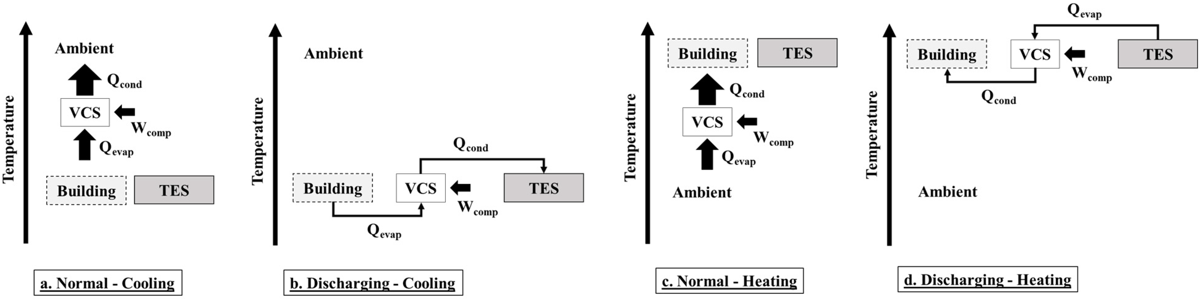
Figure 1 compares the temperature gradient for normal VCS operation (baseline system) for primary modes and TES-assisted cooling or heating. The baseline system for the primary cooling mode is shown in
Figure 1a, where the building was cooled with VCS acting as conventional air conditioning system [
24]. The VCS evaporator cooled the building air, and the condenser dispersed the heat into the ambient air. A positive temperature gradient allowed the VCS to transfer heat between the building and the ambient. A similar positive gradient is illustrated in
Figure 1c, representing a baseline system for the primary heating mode. The increasing width of arrows indicates added heat.
PCM-embedded TES can improve the building cooling and heating performance by introducing a more favorable temperature gradient for the operation of the VCS.
Figure 1b shows the TES-assisted cooling, where the condenser was coupled to the colder temperature of the TES [
24]. Therefore, to move the building’s cooling load, the VCS had a negative temperature gradient. Similarly, for the TES-assisted heating, the evaporator was coupled to the hotter temperature of the PCM and moved the heating load using a negative gradient. This gradient enabled the VCS to operate at a much higher performance compared with the baseline.
2.2. Operating Modes
The system had two primary modes: a primary cooling mode and primary heating mode. Each primary mode had four operational modes: normal mode, charging mode, discharging mode, and standby. The TES was not involved in the standby and normal modes.
Standby mode is when the HP is off, and no cooling or heating is provided. The ambient thermal loads and solar heat are gained passively during the standby cooling mode. In the normal mode, the building is cooled or heated by conventional HP operation only. In the primary cooling mode, the vapor compression cycle operates such that the condenser moves heat (Qcond) to the ambient, and the evaporator removes heat (Qevap) from the building. In the primary heating mode, the vapor compression cycle is reversed; the evaporator extracts energy from the ambient, and the condenser delivers heat to the building.
For the discharging operation in primary cooling mode, the evaporator is coupled to the building to provide space cooling, and the condenser is coupled to the TES. The heat, Qcond, is absorbed by the PCM through latent heat of melting. Likewise, for the discharging operation in primary heating mode, the HP condenser is coupled to the building to provide space heating, and the evaporator is coupled to the TES. The PCM releases heat, Qevap. The coefficient of performance (COP) is higher than in the normal operation during the discharging operation.
The PCM heat exchanger operates as the evaporator in the charging mode for cooling. The latent heat of freezing is removed from the PCM, and the condenser heat is rejected into the ambient. In the charging heating mode, the PCM operates as the condenser and absorbs Qcond through the latent heat of melting.
2.3. Component Models
The total model was a collection of submodels that operated together to maintain indoor building temperature at comfortable levels at each 1-min time step of the simulation.
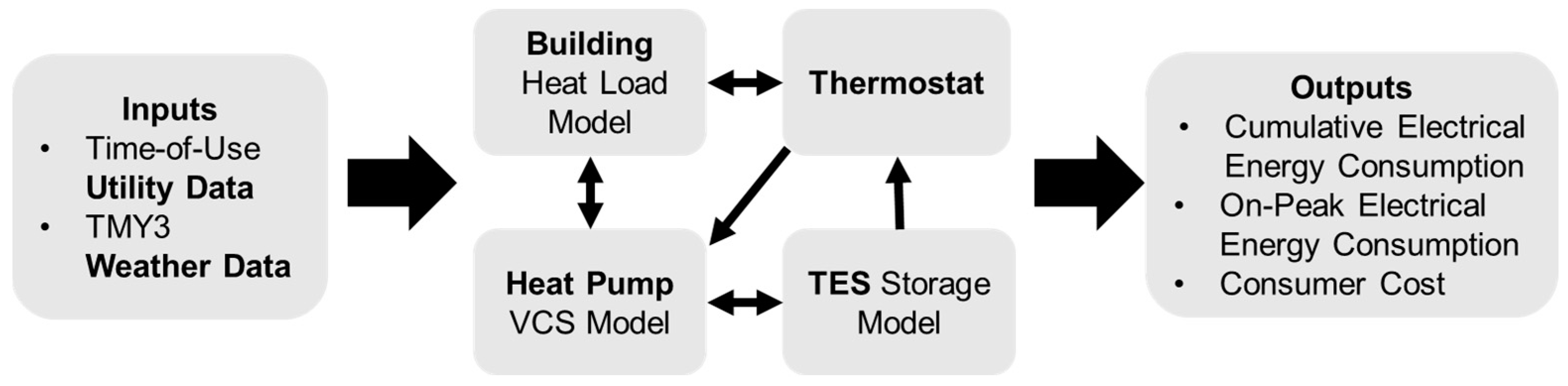
Figure 2 shows the general operating schematic of the total model and the exchange of information between submodels. All models were written in MATLAB. The following sections describe each submodel in detail.
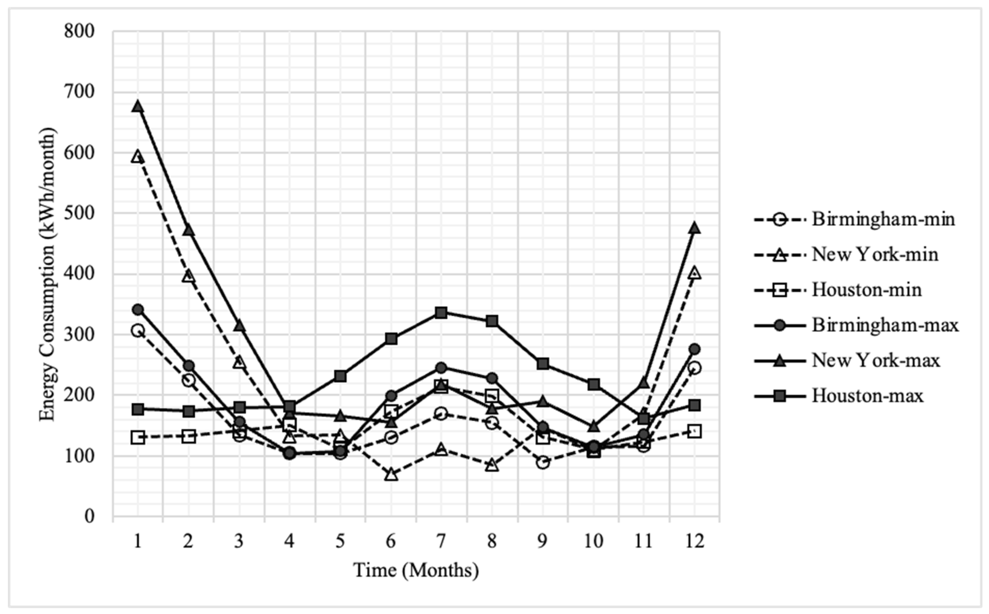
2.3.1. Weather Data
Typical meteorological year (TMY3) data was used for this analysis [
44]. This TMY3 data is hourly in its raw form with each temperature corresponding to the end of the hour. It was interpolated using a spline fit to expand to minute time step resolution. Only the ambient temperature was used. This model did not include solar irradiation or wind on the building. This information can be included in future model iterations. Considering the solar irradiation in a building model would be expected to change the building loads. Specifically, solar gain in winters would decrease the winter daytime building load (with limited effect on the electricity demand during the morning grid peak time) while solar gain in summer would increase the summer peak load. This may increase the importance of summer load and require larger cooling capacity. Potentially, our load shifting controls would then also generate higher benefits.
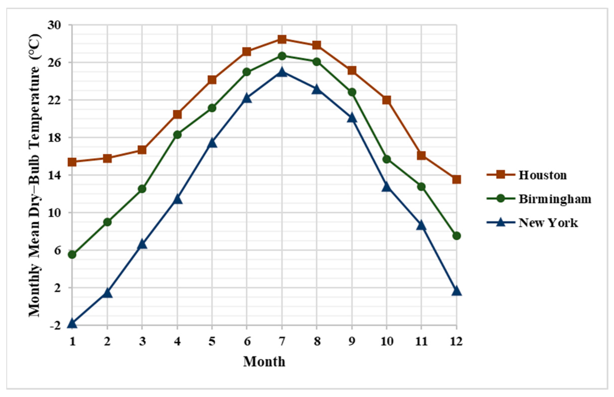
The climate locations studied were Birmingham, Houston, and New York City, corresponding to ASHRAE climate zones 3A (mixed humid), 2A (hot humid), and 4A (mixed humid), respectively [
43]. These are the representative climate zones from both cooling- and heating-dominated regions and should have different performance affected by the weather.
Figure 3 shows the average ambient dry-bulb temperature during each month for all three locations.
2.3.2. Utility Data
For this model, the on-peak periods were determined using TOU utility rates available to a residential consumer in each geographic location. TOU rates price the cost of electricity differently depending on the time of day and the month. In this analysis, only energy-based TOU rates were used—that is, the electricity is priced per kilowatt hour. Other TOU rates may provide greater information on instantaneous demand, but this factor was not considered here.
TOU rates were found for each location, and the model was run such that the on-peak times were determined when the cost of electricity was higher than the baseline.
Table 2 shows the utility cost information during 2020 for all locations, which demonstrates the disparity in electrical pricing across the United States and highlights the different financial incentives that TES may offer.
2.3.3. TES Model
The TES model was simplified for ease in analysis with only energy balance performed; no considerations were made to the inner workings of the TES system. The TES was assumed to be a heat exchanger with embedded PCM, which enabled isothermal operation. In this analysis, the TES heat exchanger was considered to have an infinite heat transfer coefficient; thus, the TES was maintained at the PCM PCT, TTES. The model was simplified to assume that Tevap and Tcond were equal to TTES during charging and discharging modes, respectively, when TES was coupled to HP.
The PCM is idealized in this model, leading to more favorable results. Zero glide and zero super cooling were assumed [
45,
46]. The glide and supercooling were neglected for simplicity. However, while the idealized PCM used in this study allowed for simplified modeling to focus on the impact of controls, there are limitations of the current model.
A recent study [
47] evaluated the energy saving and demand reduction potential of HP-TES configuration and compared the performance of ideal and realistic PCMs. The analytical analysis used ideal PCM and an HP with 5 K approach temperature, while a numerical analysis used real PCM and a more realistic HP model using ORNL’s Heat Pump Design Model (HPDM). A commercial refrigeration cooling was compared as an example. For 20 °C T
TES, 40% demand reduction and 25% energy savings were achieved using ideal PCM and an HP with 5 K approach temperature; while in the real PCM and HPDM numerical analysis case, 40% demand reduction and 20% energy savings were reported for the same T
TES of 20 °C.
Demand savings were unchanged but a 20% decrease in energy savings was observed in the real PCM case as compared to the ideal PCM. We expect a similar difference for our PCM model.
The TES stored the thermal energy desirable for the primary space conditioning mode, which defines the state of charge (SOC). At its full capacity, TES SOC is 0 in primary cooling mode and 1 in primary heating mode. TES SOC is defined as a thermal battery, where 0 refers to the PCM being fully frozen (zero usable thermal energy), and 1 indicates that it is fully melted (full of thermal energy).
Table 3 explains the SOC in different modes. During the discharging cooling mode, the TES acts as a heat sink for the HP, and TES SOC increases, thus melting the PCM. During the discharging heating mode, the TES acts as a heat source for the HP, and TES SOC decreases, thus solidifying the PCM. During the use of TES, if energy storage capacity is reached, the system will default to normal mode operation.
2.3.4. Thermostat Controls
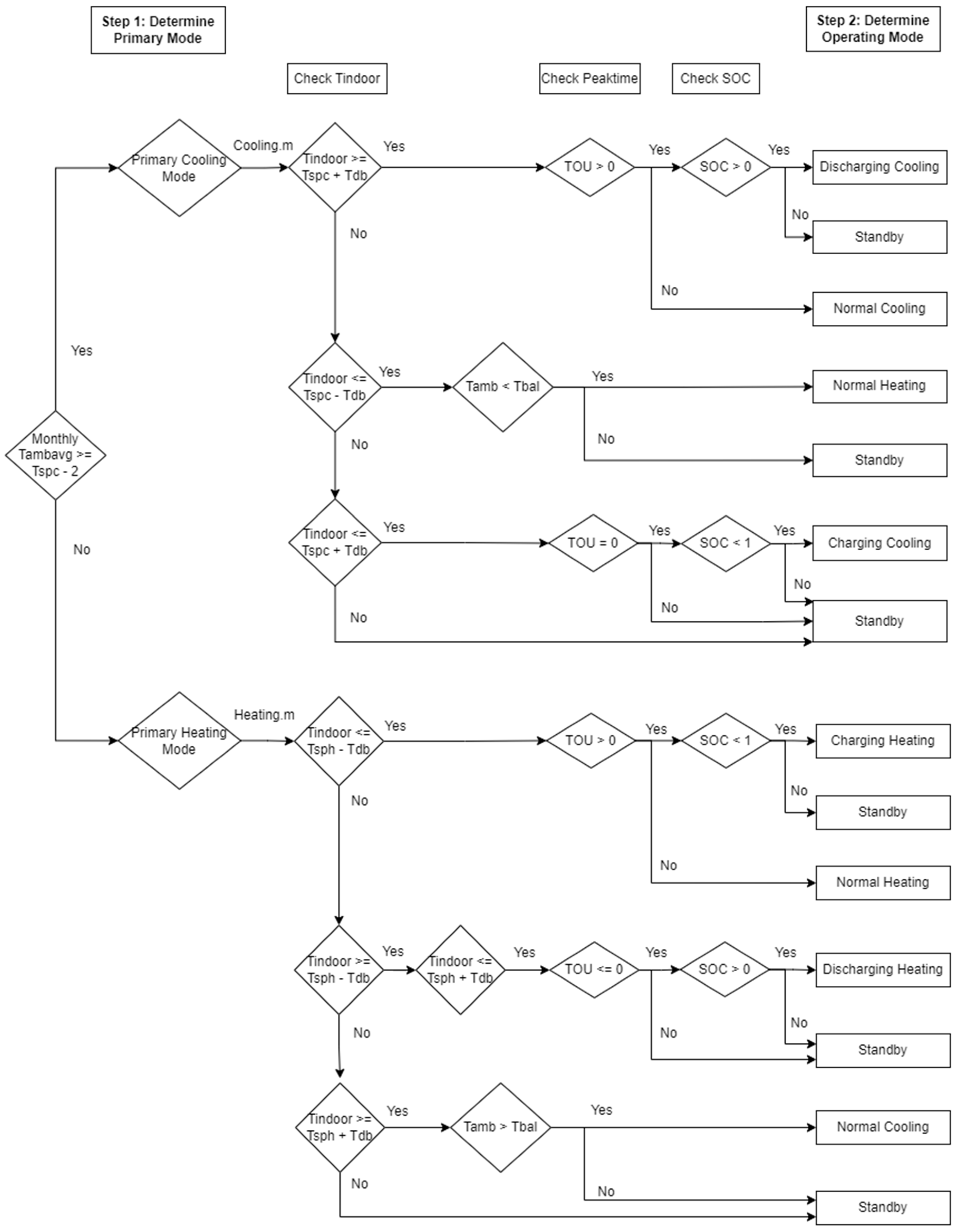
The thermostat was the core of the model and communicated information between all submodels. It determined which operating mode to use to run the TES system by monitoring the indoor temperature, TES SOC, and on-peak status. Thermostat controls were implemented in two steps. First, depending on the monthly average temperature, the thermostat determined if the building and HP were operating in primary heating mode or primary cooling mode for the given month. If the monthly average ambient temperature was greater than 2 °C above the indoor set point temperature, the system operated in primary cooling mode for that month. Otherwise, the system defaulted to primary heating mode. This step was only for convenience and did not impact the results. For the main controls to determine TES operating modes, daily values were considered, and the indoor temperature was rewritten for each minutely time step.
The building set point temperature and dead band for the primary cooling mode were 23 °C ± 0.5 °C and 20 °C ± 0.5 °C for the primary heating mode, respectively, which correspond to typical occupant behavior and ASHRAE standards for indoor climate comfort (ASHRAE 55). In the primary cooling mode, the system primed itself to reduce energy only to cool. If the indoor space needed to be heated during this mode, the TES would not be used, and the system would only use the normal heating mode. The same was true in the primary heating mode. Within these primary modes, the thermostat determined whether the heat pump or TES should be used for cooling or heating at a given time.
As shown in the controls decision tree in
Figure 4, if neither cooling nor heating was needed during off-peak time, and the TES SOC < 1, the charging mode was activated. During peak time, TES was discharged until SOC reached 0.
Table 3 shows the operating mode decisions based on indoor temperature, SOC and peak time (TOU) determination. Primary modes (column 1), as determined by monthly average temperature, had controls to determine operating modes (column 5).
Tindoor and TOU were checked at each time step, but SOC was only checked for TES modes after the first two conditions were met. This decision was the first decision made in each time step, and the appropriate information was sent to each submodel.
2.3.5. Heat Pump Model
The R410A refrigerant HP was modeled first in Engineering Equation Solver (EES) for an array of evaporator and condenser temperatures. The EES model was the same as that in previous work [
14]. HP electrical work and heat loads were calculated from the EES model and fit to the following equations.
In Equation (1), the parameter
a curve fits the density of saturated R410A vapor at the compressor suction, according to Equation (2):
The parameter
b normalizes the operation of the HP such that 7.5 kW of cooling is achieved with
Tevap = 0 °C and
Tcond = 35 °C:
The parameter
c accounts for the increase in vapor mass fraction quality entering the evaporator during isenthalpic expansion. The approximate specific heat,
cp, is 1.5 J/(g⋅K) and enthalpy of vaporization, Δ
Hg, for R410A approximately 220, as shown in Equation (4) to normalize parameter
c:
The coefficients of performance for heating and cooling were estimated using Carnot relationships and an assumed Carnot efficiency of 30%. In the case where the heat source was hotter than the heat sink, this study assumed a fixed COP. Paired with Equation (1), the heating and cooling capacity and electrical work were determined for given condensing and evaporating temperatures of the HP. During the total model run, the inputs to Tcond and Tevap were either the indoor temperature, TES temperature, or ambient temperature—as decided by the thermostat model and the operating mode.
2.3.6. Building Model
The building model was simplified to focus on HP-TES configuration. A simple, single resistor and single capacitance (1R-1C) building system were used for calculating the thermal loads on the building [
24,
48]. The heating and cooling of the building were based on daily TMY data for the individual climate regions. The resistance values were calculated based on building loads by analyzing prebuilt building models in each climate zone from EnergyPlus [
49]. The value for a typical 2500 ft
2 detached single family home in the United States was assumed as overall heat transfer coefficient: namely, UA = 0.11 kW/K. The building capacitance,
Cbuild, was calculated using Equation (7) with the balance temperature of 15 °C.
The heat load on the building from the ambient was calculated simply using the building UA and the difference between balance point temperature and ambient temperature at time
i.
The building indoor temperature was set as the set point temperature at the initial time step, and at the next time step
i + 1, it was found by Equation (6). This equation sums the heat load from the ambient and the heat load from the HP submodel.
Humidity was not considered in this model. Future analysis may improve on this building model by taking it into account.
3. Results
The PCT and TES storage capacity (EPCM) were varied parametrically to evaluate their effect on utility cost, electric consumption and peak consumption for a year. PCT was varied from 5 to 45 °C and EPCM from 5.56 to 47.2 kWh (20 to 170 MJ). Three locations in the United States were simulated.
In the following sections, results are presented for each location for annual electricity energy consumption, annual electricity consumed during peak hours and annual electric utility cost. Note that the scale on the vertical axis changes for each location. Each line in a figure corresponds to a different energy storage capacity of the TES, and winter and summer seasons are plotted separately. Baseline is the case where no TES was present, and the system operated as a conventional air source HP system.
For utility cost analysis, the TES case used the TOU tariff, and there were two baseline cases. The primary baseline was the no-TES case, where a standard utility tariff (non-TOU) was implemented; the additional baseline was the no-TES case with a TOU tariff. For each location, TOU and non-TOU tariffs are mentioned in
Table 2. The utility costs were the only energy consumption charges associated with space conditioning. This study excluded connection and base service charges.
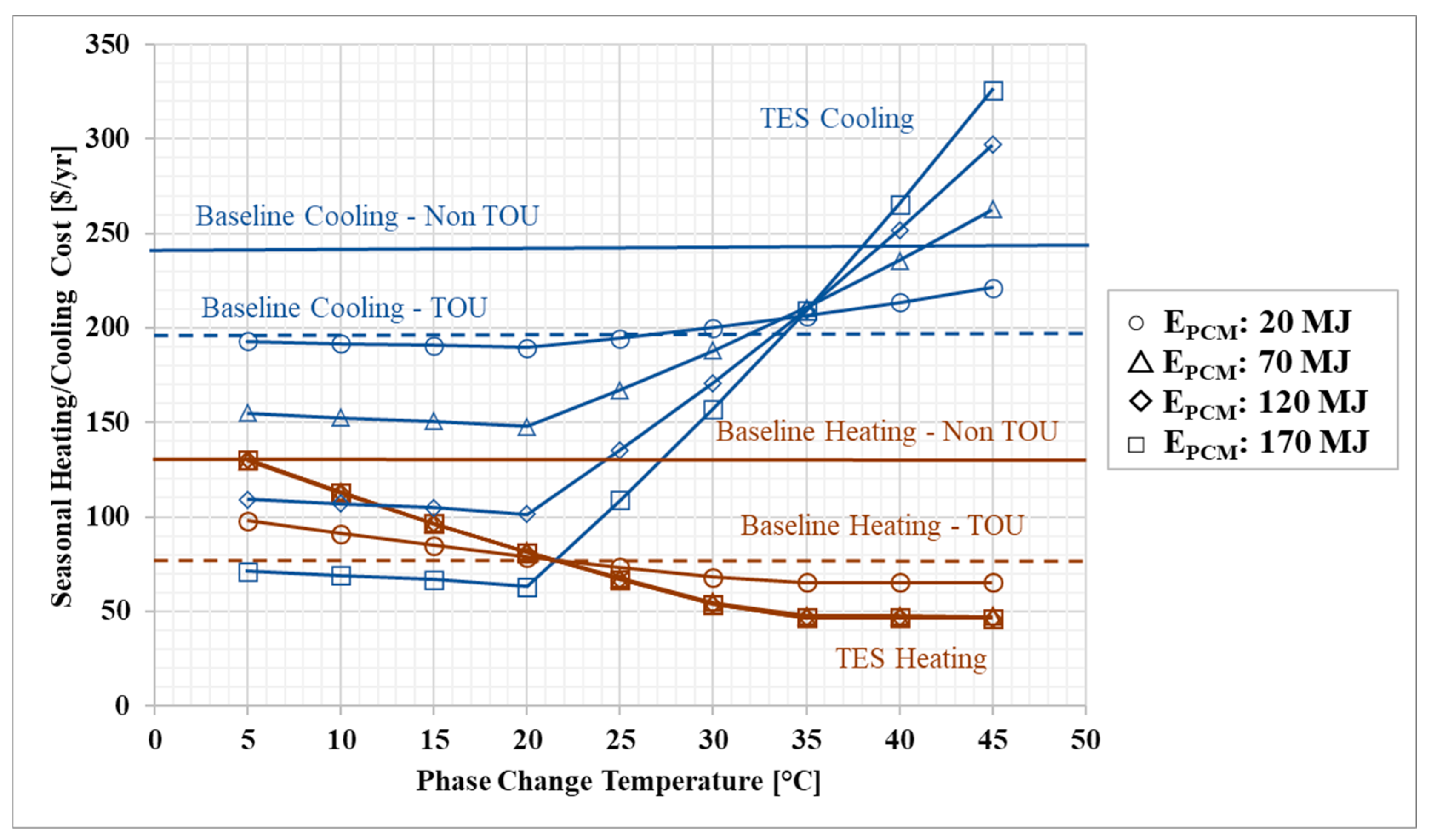
3.1. Birmingham, Alabama
Birmingham is in ASHRAE climate zone 3A (warm and humid climate).
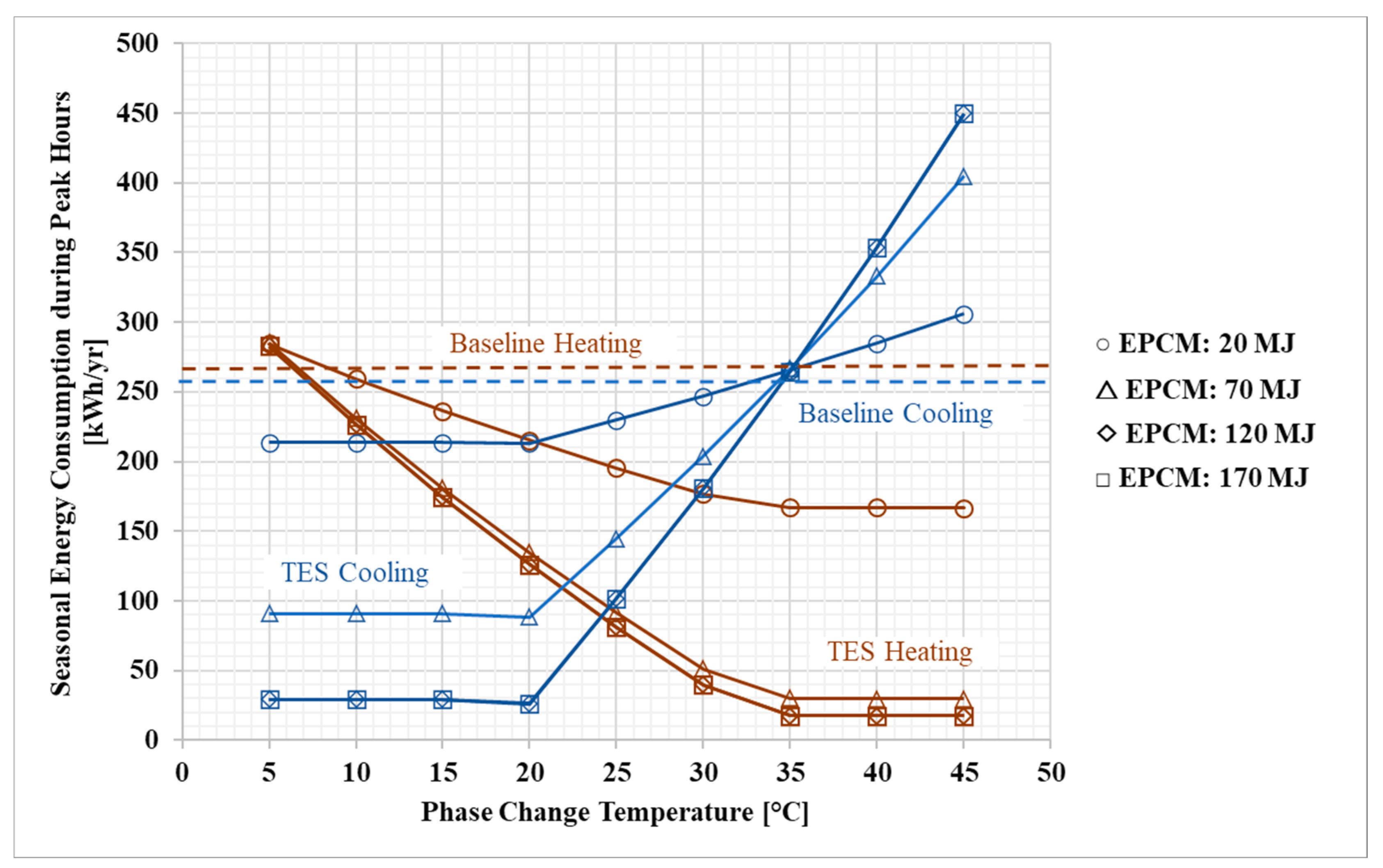
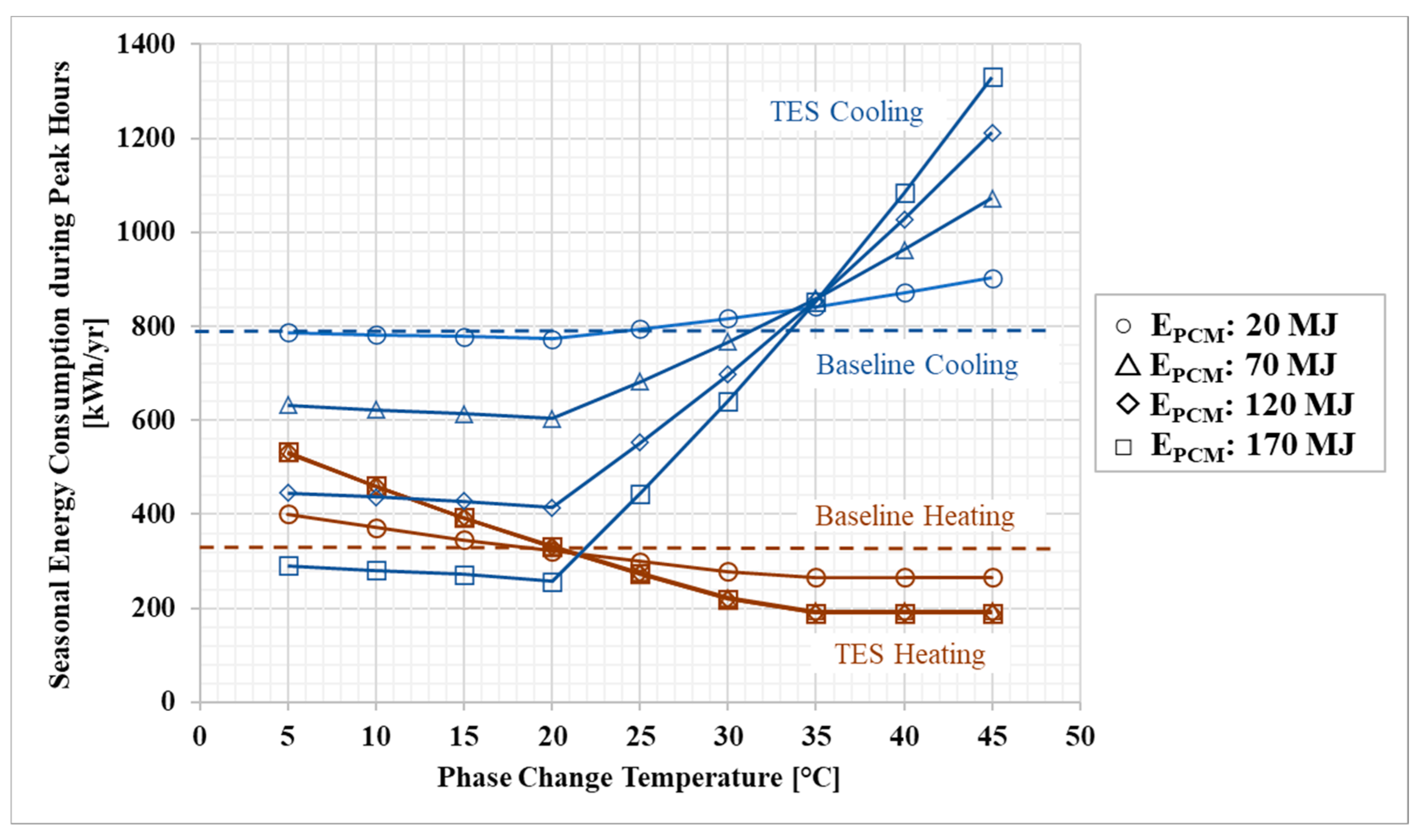
Figure 5 shows the results for electricity consumption during peak times for winter and summer (as defined by utility tariff). The winter months simulated were those in which a winter TOU tariff was active for the local utility (October–May), and the summer months simulated were the months in which a summer TOU tariff was active (June–September).
The TES with a larger storage capacity allowed for more demand shift from on-peak to off-peak hours, with diminishing returns once the TES capacity equaled the daily building thermal loads experienced during the most extreme ambient conditions.
At PCT below 20 °C for cooling, the peak energy consumption was consistent. This consistency was because the study assumed a constant COP when the source was hotter than the sink. Above 20 °C shows decreasing benefits as the PCM temperature increased, and as it approached 35 °C, the TES consumed more energy than the baseline. This increase was because the control strategy only depended on peak time, which was defined by the TOU rate; it did not depend on ambient weather. At 35 °C, the peak energy consumption was the same regardless of the size. This lack of change was because 32–35 °C was the average ambient temperature during summer peak hours, and discharging TES for cooling at 32–35 °C was expected to be equivalent to or worse than the baseline. As PCT further increased, there was a penalty to discharge the system when TES became even hotter than the ambient; that is, when the TES consumed more energy than the baseline. Hence, TES was not effective if PCT was closer to or hotter than the ambient. PCT of 20 °C saved maximum energy for the cooling season, and 35 °C was ideal for heating.
Figure 5 shows seasonal results. Throughout the year, using a single PCM with 20 °C PCT and TES with 47.2 kWh (170 MJ) storage capacity, the annual reduction in energy consumption during on-peak hours was 70.5% (517 kWh/year baseline vs. 152 kWh/year with TES). In the TES case, the cumulative energy consumption during on-peak hours was 152 kWh/year (not shown in figure). Compared with the baseline, 365 kWh/year energy consumption was shifted from on-peak to off-peak hours.
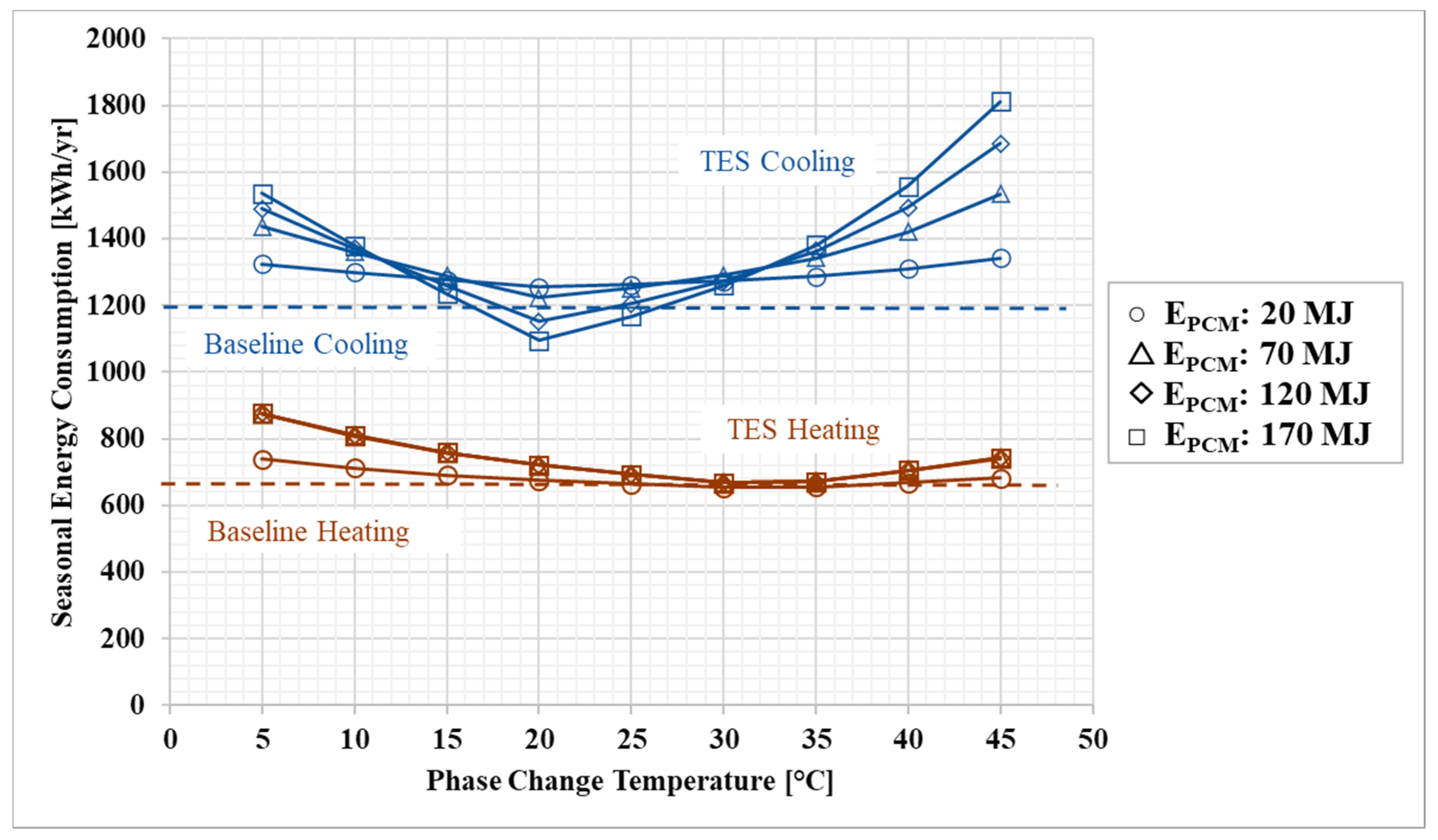
Figure 6 shows summer and winter energy consumption associated with space conditioning as a function of PCT for different TES sizes. Percent cooling energy savings were highest with a PCT of 20 °C and energy storage capacity of 33.3 kWh (120 MJ). During summers, at 20 °C, the smallest TES consumed more energy than the baseline. This increase was because of the suboptimal rule-based control strategy, which did not account for ambient temperature in charging mode decision-making. TES was charging even when it was hot outside, and that reduced the charging–discharging cycle efficiency of the TES, resulting in more energy consumption. This effect was less prominent in a larger TES because it took longer for the larger TES to charge. For the cooling season, a larger TES experienced the charging process further into the evening when the ambient temperature naturally dropped. Cooling energy savings were observed only when the PCT was between 15 and 25 °C. It is unfavorable to use TES at temperatures far from the indoor temperature. The smallest 5.56 kWh (20 MJ) TES consumed less energy than the larger TES at extreme temperatures because the smallest did not get used as much.
The heating results are more consistent and do not deviate as much at extreme temperatures because Birmingham is a cooling-dominated climate. The ambient temperatures were not as extreme for frequent unfavorable charging, and even 70 MJ TES in this case could fulfil the heating demand at 35 °C PCT.
Annual energy savings (not shown in figure) for a single PCM with a PCT of 20 °C at an energy storage capacity of 33.3 kWh (120 MJ) was 5.4% (2036 kWh/year baseline vs. 1925 kWh/year with TES). Annual energy savings in general were much less than peak savings because of the increased energy consumption during off-peak times required to recharge the TES. This result is consistent with previous studies.
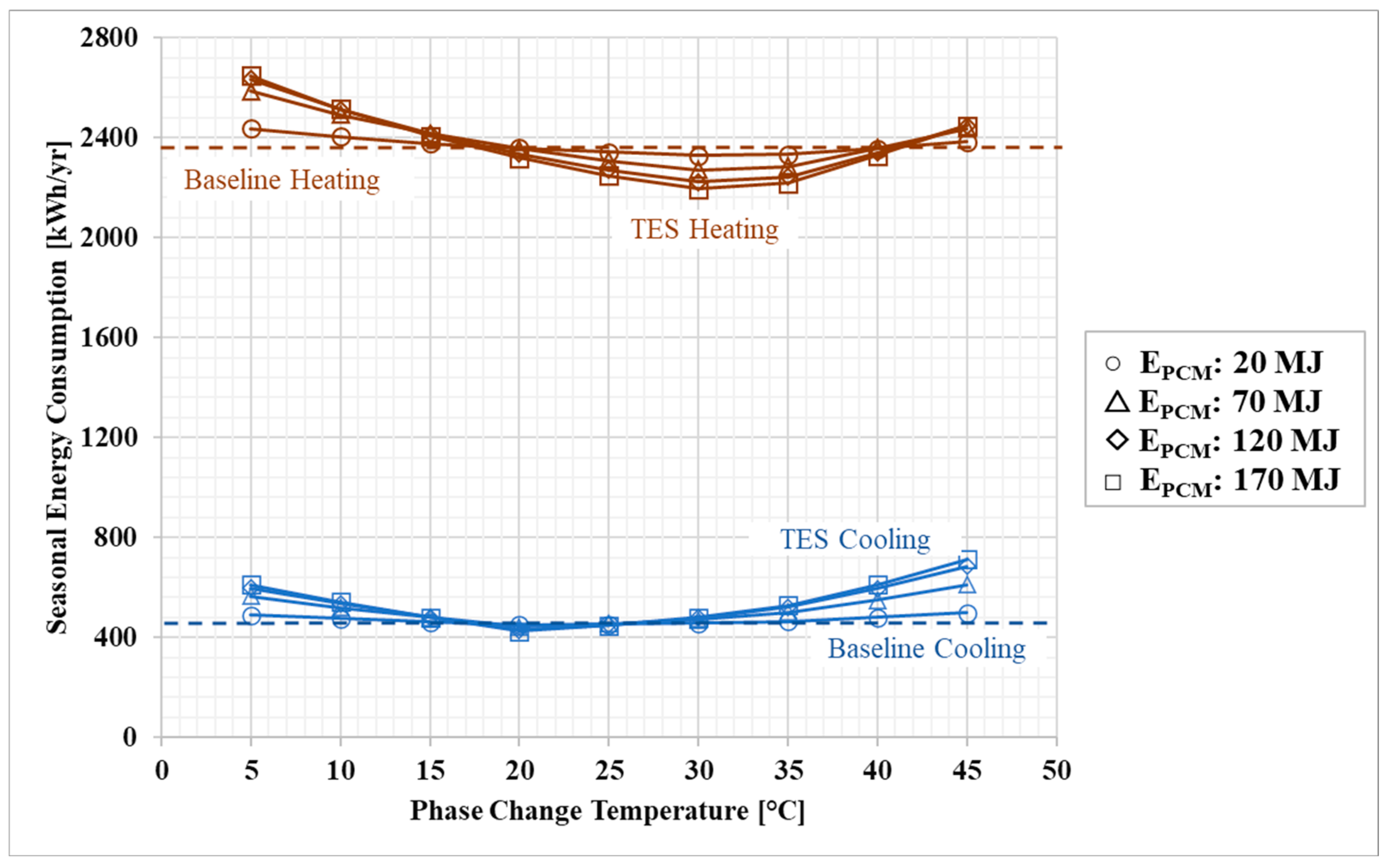
The heating and cooling cost of the integrated HP and TES system in Birmingham is shown in
Figure 7. TES used the TOU rate and was compared against TOU and non-TOU baselines. The trend for TES is similar to the peak energy consumption for summers, except the cost slightly rose again below 20 °C. This increase was because more off-peak energy below 20 °C meant an increase in utility payment. For winters, the off-peak price was greater than in summers; thus, the savings were more significant.
Figure 7 shows that TOU baselines were already saving cost as compared with non-TOU baselines. For the winter baseline case, more cost was saved using a TOU tariff. The difference between the primary baseline and TOU baseline is huge because on-peak and off-peak TOU rates were less than the standard rate (non-TOU) in winters (
Table 2). For summer, the primary baseline saved more cost than the TOU baseline because the on-peak TOU rate was much higher than the standard non-TOU rate (difference of 15.48 ¢/kWh).
Figure 7 shows seasonal results. Total annual results are not shown. The annual TES cost was
$141/year (a saving of
$111/year compared with the baseline). The 43.9% cost savings were achieved by using TES at 20 °C PCT and 33.3 kWh (120 MJ) energy storage capacity under the TOU rate structure with
$0.2/kWh price differential between on-peak and off-peak times during summers and
$0.02/kWh during winters. For the baseline system, the annual energy cost would have been
$252.7/year.
3.2. New York City, New York
New York City is in ASHRAE climate zone 4A, a mixed humid climate. It is considered a subtropical continental climate with large variations between summer and winter.
Figure 8 shows the results for electricity consumption during peak times for winter and summer (as defined by the utility tariff). Winter months were when the winter TOU tariff was active (October–May), and summer months were those in which the summer TOU tariff was active (June–September). The trend is similar to peak energy results in Birmingham. Maximum savings are observed at PCT 20 °C for the summer season and 35 °C for heating, with a 170 MJ storage capacity for both cases. TES was not effective when PCT was far from these values.
Figure 8 shows seasonal results optimized at different PCT and
EPCM for winter and summers. The annual results were calculated by performing parametric analysis for the whole year and finding the PCT and
EPCM that delivered maximum annual reduction in the cumulative energy consumption during on-peak hours. Peak energy consumption of 53% was reported, achieved by using a TES with 47.2 kWh (170 MJ) storage capacity and 30 °C PCT under the TOU tariff. The on-peak TOU rates in New York are much higher than others. The cumulative energy consumption during on-peak hours was 627 kWh, and for the baseline, the minimum on-peak annual energy consumed was 1344 kWh/year. Compared to the baseline, 717 kWh/year energy consumption was shifted from on-peak to off-peak hours.
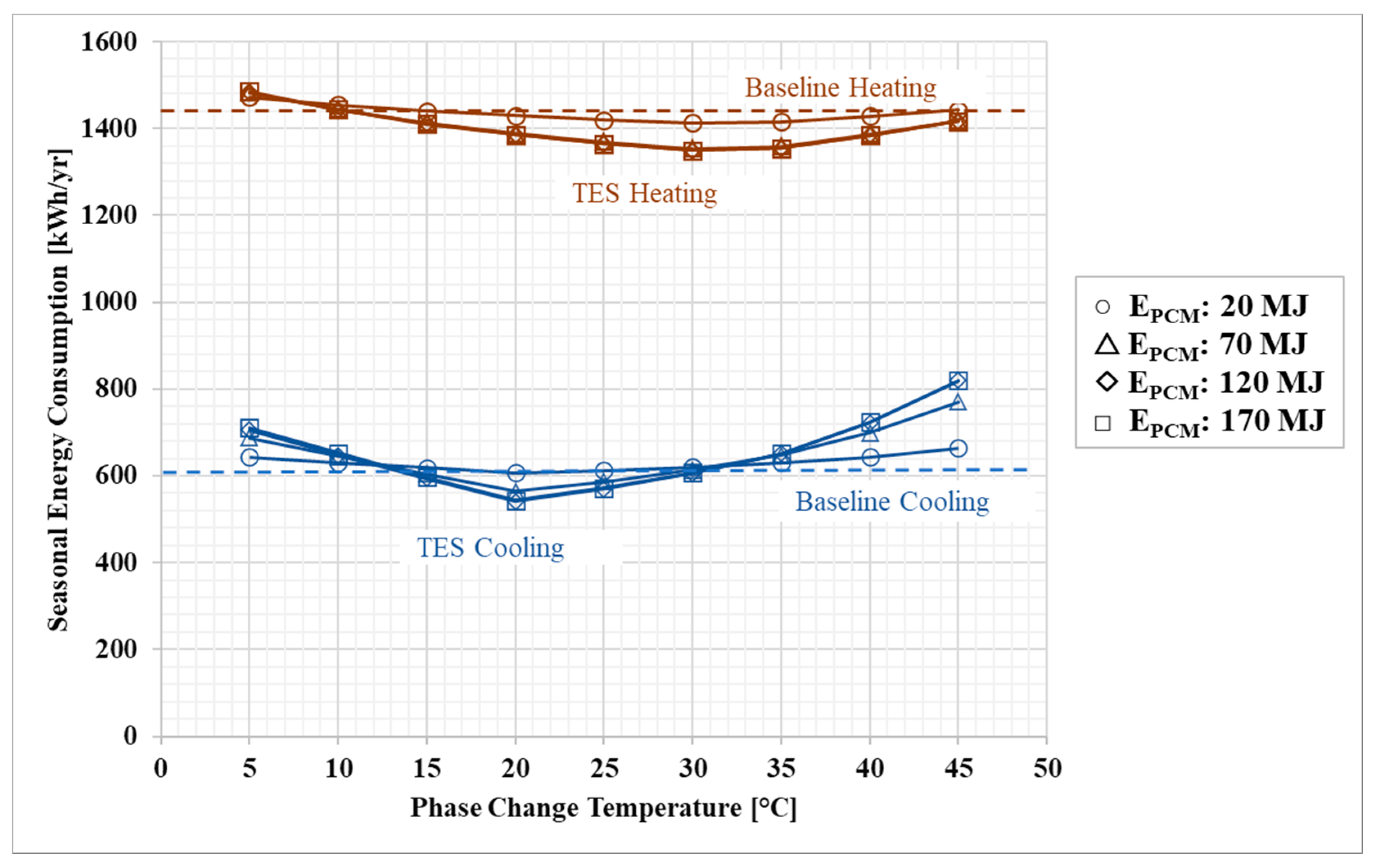
Figure 9 shows seasonal energy consumption associated with space conditioning against PCT for different TES sizes. Cooling energy savings were both insignificant—0.98%—and achieved only with a PCT of 20 °C, while heating savings (6.9%) were achieved with PCT 30 °C, both at an energy storage capacity of 170 MJ. For heating, TES energy savings were observed when the PCT was between 25 and 35 °C. It was unfavorable to use TES otherwise.
The maximum annual energy savings (not shown in figure) for New York City were approximately 3.9% (2675 kWh/year vs. 2785 kWh/year) with a PCT of 30 °C and energy storage capacity of 47.2 kWh (170 MJ).
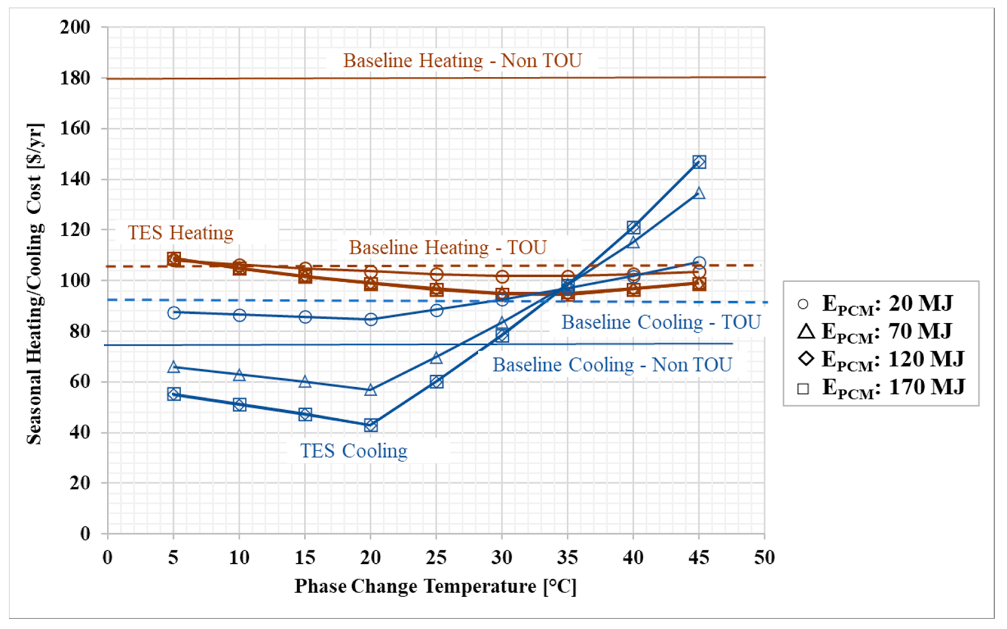
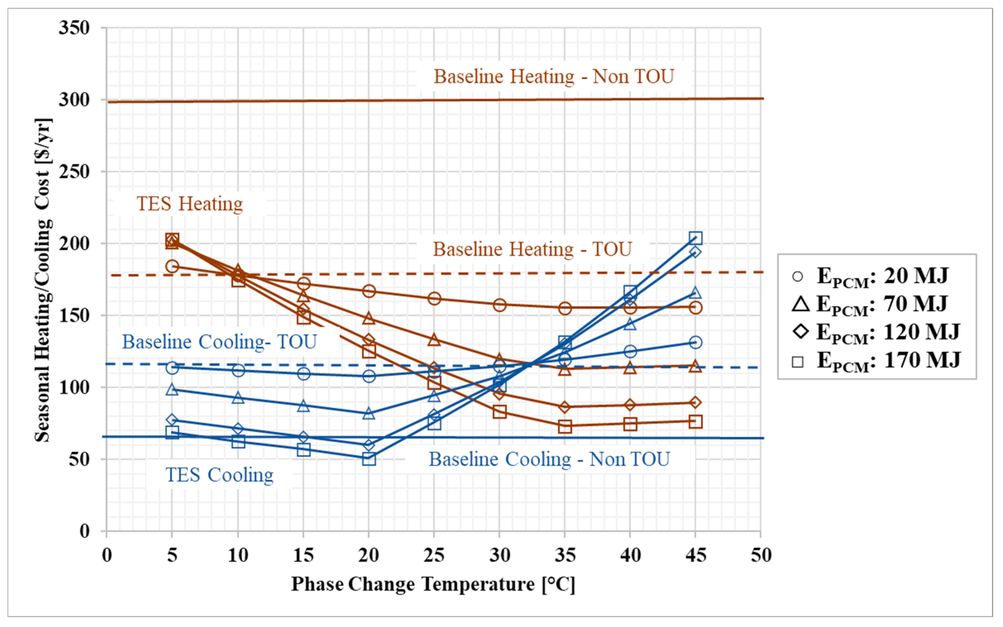
Figure 10 shows the seasonal heating and cooling cost of the integrated HP and TES system in New York City. Maximum TES savings were achieved using 170 MJ
EPCM at 35 °C in winters and 20 °C in summers. TES and TOU baselines meet at 32 °C in summers and 10 °C in winters, which indicates that discharging TES at these PCTs is the same as normal HP operation, yielding no savings.
For winters, TOU baselines saved more cost compared with non-TOU baselines. The TOU off-peak rate was very cheap, and it was almost free electricity at 1.5 ¢/kWh (
Table 2). For summer, the primary baseline saved more cost than the TOU baseline because the on-peak TOU rate was much higher (40.1 ¢/kWh) than the standard non-TOU rate (14.6 ¢/kWh).
Annual savings of 35% were achieved at 30 °C PCT and 170 MJ EPCM. TES cost was $185/year under the TOU rate structure. Without the TOU rate structure, the minimum peak annual energy cost was $287.5/year.
3.3. Houston, Texas
Houston is a hot, humid climate zone, categorized as 2A. In these plots, winter was November through March, and summer was April through October, as defined by historical average climate in Houston [
50].
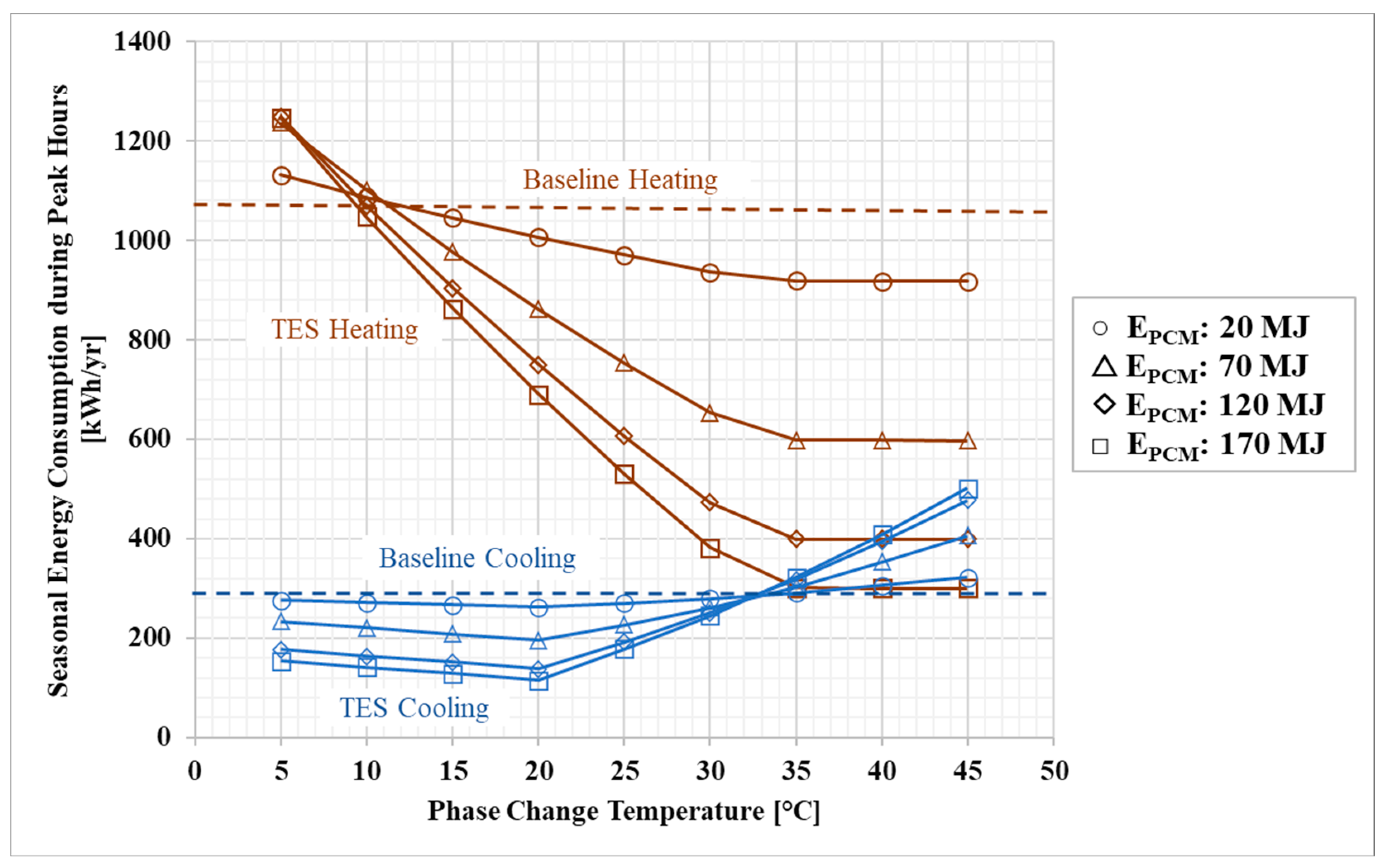
Figure 11 shows peak energy consumption during winter and summer for Houston. The notable cooling energy savings were observed at PCT 20 °C and
EPCM of 170 MJ. For the winter season, even a 70 MJ storage capacity was enough to meet the load, and maximum savings were achieved at PCT 35 °C. Baseline heating and TES met at 20 °C, which means that discharging TES for heating at 20 °C would be the same as using an HP in normal mode. This was also the case for cooling at 35 °C. The TES consumption with PCT increased at far beyond these values.
The maximum annual reduction (not shown in figure) in the cumulative energy consumption during on-peak hours was 47%, achieved by using a TES with 47.2 kWh (170 MJ) storage capacity and 20 °C PCT under the TOU tariff. The cumulative energy consumption during on-peak hours was 588 kWh. For the baseline system, the minimum on-peak annual energy consumed was 1120 kWh/year without the TOU tariff. Energy consumption of 531.9 kWh/year was shifted from on-peak to off-peak hours.
Figure 12 shows seasonal results optimized at different PCT and
EPCM for winter and summer. The minimum annual energy consumption (not shown in figure) was 1816 kWh/year with a PCT of 20 °C and energy storage capacity of 47.2 kWh (170 MJ). For the baseline case, energy consumption was 1848 kWh/year. Annual energy savings were observed only when the PCT was between 20 and 35 °C. The energy savings were 1.75%, which is lower than the savings at other locations. Heating energy savings during winters in the New York City case made a huge difference to the results. Houston, on the other hand, is a cooling-dominated, humid climate with very short and mild winters, yielding less significant heating energy savings.
Figure 13 shows the seasonal heating and cooling cost of the integrated HP and TES system in Houston. Maximum TES savings were achieved using 170 MJ EPCM at 35 °C in winters and 20 °C in summers. TES and TOU baselines met at 35 °C in summers and 20 °C in winters, which indicates that discharging TES at these PCTs was the same as for normal heat pump operation, yielding no savings.
For both seasons, TOU baselines saved more cost compared with non-TOU baselines because off-peak energy was free in Houston under the TOU tariff by Gexa Energy (
Table 2).
Figure 13 shows seasonal results. The annual minimum on-peak annual energy cost of the integrated HP and TES system in Houston was
$144/year with 20 °C PCT under the TOU rate structure. Without the TOU rate structure, the minimum peak annual energy cost was
$274.6/year, corresponding to 47% savings.
4. Discussion
This study focused on evaluating the indirect HP-TES configuration using simple, rule-based controls with time-based, predefined utility rates. For that reason, the building model and control strategy were simplified.
Figure 14 shows monthly total energy consumption for all three locations. The minimum refers to the values obtained at optimum PCTs (20 °C for summers and 30 °C for winters). The maximum values refer to those found at extreme PCTs (45 °C for summers and 5 °C for winters). The consumption is highest for New York during winters and for Houston during summers. Even though cooling loads for Birmingham are higher than the heating loads, they are comparatively moderate.
In a previous study [
24], 20% energy savings were achieved by using similar control strategies and configuration to those used for an ice storage system in Fresno, California (ASHRAE climate zone 3B). The TES in the previous study was simulated for 1 week, and only the cooling mode was studied. The total energy consumption savings were smaller in the current study. One reason for this decrease is that the week simulated in Fresno in the previous study [
24] had particularly large diurnal temperature swings, and the year-long simulations in this study had smaller average diurnal swings. TES can provide more energy savings for climate locations where the daily diurnal temperature swing is larger than the difference between indoor and PCM temperature.
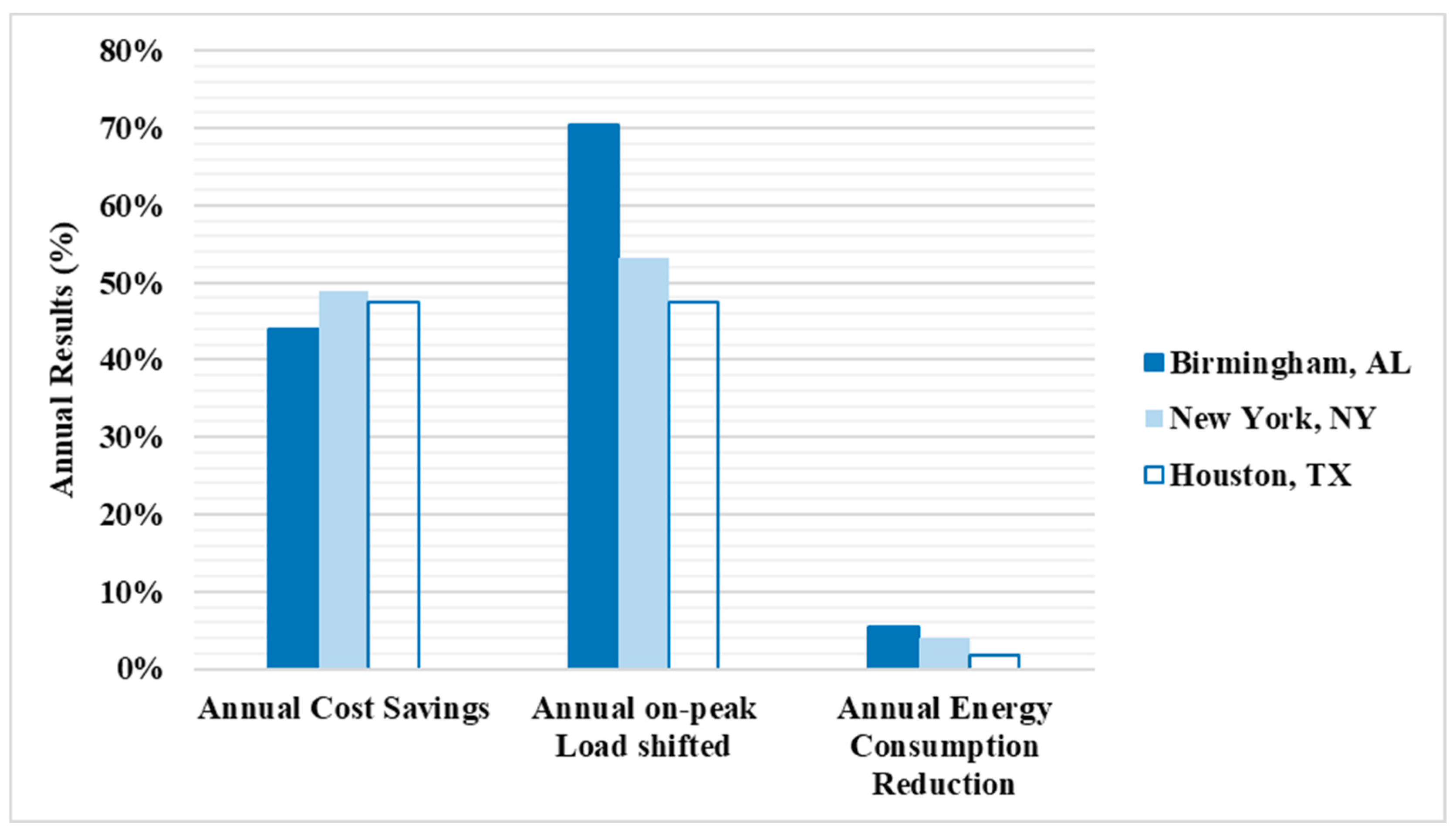
The annual results are shown in
Table 4 and
Figure 15. To meet the high cooling demand in Birmingham and Houston, the optimized PCT was 20 °C for maximum annual cost savings and peak electric demand reduction. For the New York City case, the optimum PCT was 30 °C because of the high heating load.
Energy savings were highly dependent on the ambient temperature and diurnal swing, while the cost savings and peak load shifted were driven by the peak time and heating and cooling demand for each climate location studied. It can be concluded that higher savings are expected in warmer areas where cooling demands dominate.
We only analyzed PCT from 0 to 45 °C with a resolution of 5 °C, and this is a limitation of this study. If the optimum lay between 20 and 25 °C, for example, that would not show up in our assessment.
An important controls shortcoming was identified in this study. PCM was used for discharging even if the ambient temperature was not favorable. For instance, if the PCT was lower than the ambient temperature, extracting heat from the TES resulted in more electricity consumption to meet the heating load as compared with the normal mode (i.e., extracting heat from warmer ambient air). Thus, predictive weather data should be included in control strategies for future work to optimize TES operation.
TES systems with larger storage capacities were shown to have a narrower acceptable PCT range because the adverse effects of this suboptimal control strategy became more pronounced at extreme PCTs. In future work, the control strategy should be improved to take advantage of the daily ambient temperature swing.
5. Conclusions
An HP-integrated TES was modeled in a simple configuration to determine the PCT and storage capacity that maximized energy savings, cost savings, and peak shifting for select residential building types. Three TES systems were modeled and compared with a baseline for different climate zones in the United States: Birmingham, Houston, and New York City. The simple, rule-based TES controls were designed to shift the load from on-peak to off-peak hours based on TOU utility tariffs available to residential customers in these locations. Very simple models of the HP, TES, and building were used to focus on evaluating the potential energy and cost savings and grid benefits of this HP-TES configuration. The best TES storage capacity and melting temperature were calculated for each case.
Birmingham and Houston are cooling-dominated climates, and 20 °C was found to be the best melting temperature for annual energy and cost savings, as well as demand shift. New York City saw the largest energy savings and demand shift at 30 °C because the system needed to meet a high heating demand. The highest energy savings of 5.4% and maximum peak load shifting of 70% compared with the baseline HP were observed in the Birmingham case. Maximum energy cost savings of 48.9% compared with the baseline ASHP were achieved in New York City. The energy cost savings and peak load shifted were driven by the peak time and heating and cooling demand for each climate location studied. TES with larger storage capacity allowed for more demand shift, with diminishing returns once the TES capacity equaled the daily building thermal loads experienced during the most extreme ambient conditions.
The scope of this work is limited to space conditioning in typical single-family residential buildings of U.S. and the building model is simplified. A more sophisticated model will be implemented in future iterations of this work and is expected to change the building loads. Three climate zones have been analyzed in this work, but in future, a comprehensive analysis will be performed on more locations to represent more variations in climates and to generalize expected results. For the TES model, an arbitrary idealized PCM is used and a range of PCTs is analyzed with a difference of 5 °C only. Future work will consider more values in between for optimization and a more robust TES model. Future models will also improve the control strategy and consider more variables such as ambient temperature and diurnal swing.
Author Contributions
Conceptualization, S.S., N.K. and K.R.G.; Methodology, S.S., J.H., N.K. and K.R.G.; Software, N.K. and B.C.; Validation, S.S., J.H., N.K. and B.C.; Formal analysis, S.S., J.H. and N.K.; Investigation, S.S., J.H. and N.K.; Data curation, S.S., J.H. and N.K.; Writing—original draft, S.S., J.H. and N.K.; Writing—review & editing, J.H., N.K., B.C., X.L., T.J.L. and K.R.G.; Visualization, S.S., N.K., X.L. and K.R.G.; Supervision, K.R.G.; Project administration, K.R.G.; Funding acquisition, K.R.G. All authors have read and agreed to the published version of the manuscript.
Funding
This work was sponsored by the U. S. Department of Energy’s Building Technologies Office under Contract No. DE-AC05-00OR22725 with UT-Battelle, LLC.
Data Availability Statement
Acknowledgments
This research used resources at the Building Technologies Research and Integration Center, a DOE Office of Science User Facility operated by the Oak Ridge National Laboratory. The authors would also like to acknowledge Antonio Bouza, Technology Manager–HVAC&R, Water Heating, and Appliance, U.S. Department of Energy Building Technologies Office. The authors would like to acknowledge Kyle Gluesenkamp for supervising this research, and co-authors for their contributions. The authors would also like to acknowledge Bredesen Center at University of Tennessee for academic support.
Conflicts of Interest
The authors declare no conflict of interest. The funders had no role in the design of the study; in the collection, analyses, or interpretation of data; in the writing of the manuscript; or in the decision to publish the results.
References
- U.S. Energy Information Administration—EIA. Annual Energy Outlook. 2020. Available online: https://www.eia.gov/outlooks/aeo/ (accessed on 19 April 2020).
- Goetzler, B.; Guernsey, M.; Kassuga, T. Grid-Interactive Efficient Buildings Technical Report Series: HVAC. Water Heating; Appliances; and Refrigeration. 2019. Available online: https://www.osti.gov/biblio/1577966/%20http:/files/87/Neukomm%20et%20al.%20-%202019%20-%20Grid-Interactive%20Efficient%20Buildings%20Technical%20Rep.pdf (accessed on 19 May 2021).
- Center for Sustainable Systems. Residential Buildings Factsheet. 2021. Available online: https://css.umich.edu/publications/factsheets/built-environment/residential-buildings-factsheet (accessed on 16 June 2022).
- U.S. Energy Information Administration—EIA. Nearly 90% of U.S. Households Used Air Conditioning in 2020. Residential Energy Consumption Survey. Available online: https://www.eia.gov/todayinenergy/detail.php?id=52558&src=%E2%80%B9%20Consumption%20%20%20%20%20%20Residential%20Energy%20Consumption%20Survey%20(RECS)-b1 (accessed on 16 June 2022).
- Arteconi, A.; Mugnini, A.; Polonara, F. Energy flexible buildings: A methodology for rating the flexibility performance of buildings with electric heating and cooling systems. Appl. Energy 2019, 251, 113387. [Google Scholar] [CrossRef]
- Chen, Y.; Xu, P.; Gu, J.; Schmidt, F.; Li, W. Measures to improve energy demand flexibility in buildings for demand response (DR): A review. Energy Build. 2018, 177, 125–139. [Google Scholar] [CrossRef]
- Jensen, S.Ø.; Marszal-Pomianowska, A.; Lollini, R.; Pasut, W.; Knotzer, A.; Engelmann, P.; Stafford, A.; Reynders, G. IEA EBC Annex 67 Energy Flexible Buildings. Energy Build. 2017, 155, 25–34. [Google Scholar] [CrossRef] [Green Version]
- Junker, R.G.; Azar, A.G.; Lopes, R.A.; Lindberg, K.B.; Reynders, G.; Relan, R.; Madsen, H. Characterizing the energy flexibility of buildings and districts. Appl. Energy 2018, 225, 175–182. [Google Scholar] [CrossRef]
- Sarkar, M. How American Homes Vary by the Year They Were Built; US Census Bureau: Washington, DC, USA, 2011. Available online: http://www.census.gov/const/www/charindex.html (accessed on 19 May 2021).
- Sultan, S.; Gluesenkamp, K.R. The State of Art of Heat-Pump integrated Thermal Energy Storage for Demand Response. IEA Heat Pump Technol. Mag. 2021, 40, 27–30. [Google Scholar] [CrossRef]
- Sultan, S.; Turnaoglu, T.; Akamo, D.; Hirschey, J.; Liu, X.; Laclair, T.; Gluesenkamp, K. PCM Material Selection for Heat Pump Integrated with Thermal Energy Storage for Demand Response in Residential Buildings. In Proceedings of the International High Performance Buildings Conference, West Lafayette, IN, USA, 14 July 2022; Available online: https://docs.lib.purdue.edu/ihpbc/427 (accessed on 19 January 2023).
- Chavan, S.; Rudrapati, R.; Manickam, S. A comprehensive review on current advances of thermal energy storage and its applications. Alex. Eng. J. 2022, 61, 5455–5463. [Google Scholar] [CrossRef]
- Kurdi, A.; Almoatham, N.; Mirza, M.; Ballweg, T.; Alkahlan, B. Potential Phase Change Materials in Building Wall Construction—A Review. Materials 2021, 14, 5328. [Google Scholar] [CrossRef]
- Amberkar, T.; Mahanwar, P. Thermal energy management in buildings and constructions with phase change material-epoxy composites: A review. Energy Sources Part A Recovery Util. Environ. Eff. 2023, 45, 727–761. [Google Scholar] [CrossRef]
- Rahman, M.M.; Habib, M.A. Energy storage using phase change materials—Challenges and opportunities for power savings in residential buildings. AIP Conf. Proc. 2022, 2681, 020054. [Google Scholar] [CrossRef]
- Sepehri, A. Introduction and Literature Review of Building Components with Passive Thermal Energy Storage Systems. In Green Energy Technology; Springer: Cham, Switzerland, 2022; pp. 1–18. [Google Scholar] [CrossRef]
- Wang, X.; Zhang, Y.; Xiao, W.; Zeng, R.; Zhang, Q.; Di, H. Review on thermal performance of phase change energy storage building envelope. Chin. Sci. Bull. 2009, 54, 920–928. [Google Scholar] [CrossRef] [Green Version]
- Thambidurai, M.; Panchabikesan, K.; Mohan, N.K.; Ramalingam, V. Review on phase change material based free cooling of buildings-The way toward sustainability. J. Energy Storage 2015, 4, 74–88. [Google Scholar] [CrossRef]
- Akeiber, H.; Nejat, P.; Majid, M.Z.A.; Wahid, M.A.; Jomehzadeh, F.; Famileh, I.Z.; Calautit, J.K.; Hughes, B.R.; Zaki, S.A. A review on phase change material (PCM) for sustainable passive cooling in building envelopes. Renew. Sustain. Energy Rev. 2016, 60, 1470–1497. [Google Scholar] [CrossRef]
- Souayfane, F.; Fardoun, F.; Biwole, P.H. Phase change materials (PCM) for cooling applications in buildings: A review. Energy Build. 2016, 129, 396–431. [Google Scholar] [CrossRef]
- De Gracia, A.; Cabeza, L.F. Phase change materials and thermal energy storage for buildings. Energy Build. 2015, 103, 414–419. [Google Scholar] [CrossRef] [Green Version]
- Zhang, Y.; Zhou, G.; Lin, K.; Zhang, Q.; Di, H. Application of latent heat thermal energy storage in buildings: State-of-the-art and outlook. Build. Environ. 2007, 42, 2197–2209. [Google Scholar] [CrossRef]
- Dong, J.; Shen, B.; Munk, J.; Gluesenkamp, K.R.; Laclair, T.; Kuruganti, T. Novel PCM Integration with Electrical Heat Pump for Demand Response. In Proceedings of the IEEE Power and Energy Society General Meeting, Atlanta, GA, USA, 4–8 August 2019. [Google Scholar] [CrossRef]
- Sultan, S.; Hirschey, J.; Gluesenkamp, K.; Graham, S. Analysis of Residential Time-of-Use Utility Rate Structures and Economic Implications for Thermal Energy Storage. 2021, pp. 1–10. Available online: https://docs.lib.purdue.edu/cgi/viewcontent.cgi?article=1369&context=ihpbc (accessed on 31 August 2021).
- Chaiyat, N.; Kiatsiriroat, T. Energy reduction of building air-conditioner with phase change material in Thailand. Case Stud. Therm. Eng. 2014, 4, 175–186. [Google Scholar] [CrossRef] [Green Version]
- Long, J.Y.; Zhu, D.S. Numerical and experimental study on heat pump water heater with PCM for thermal storage. Energy Build. 2008, 40, 666–672. [Google Scholar] [CrossRef]
- Mosaffa, A.H.; Farshi, L.G. Exergoeconomic and environmental analyses of an air conditioning system using thermal energy storage. Appl. Energy 2016, 162, 515–526. [Google Scholar] [CrossRef]
- Bruno, F.; Tay, N.H.S.; Belusko, M. Minimising energy usage for domestic cooling with off-peak PCM storage. Energy Build. 2014, 76, 347–353. [Google Scholar] [CrossRef]
- Waqas, A.; Kumar, S. Phase change material (Pcm)-based solar air heating system for residential space heating in winter. Int. J. Green Energy 2013, 10, 402–426. [Google Scholar] [CrossRef]
- Arkar, C.; Medved, S. Free cooling of a building using PCM heat storage integrated into the ventilation system. Sol. Energy 2007, 81, 1078–1087. [Google Scholar] [CrossRef]
- Waqas, A.; Kumar, S. Utilization of latent heat storage unit for comfort ventilation of buildings in hot and dry climates. Int. J. Green Energy 2011, 8, 1–24. [Google Scholar] [CrossRef]
- Waqas, A.; Ali, M.; Din, Z.U. Performance analysis of phase-change material storage unit for both heating and cooling of buildings. Int. J. Sustain. Energy 2017, 36, 379–397. [Google Scholar] [CrossRef]
- Evola, G.; Marletta, L.; Sicurella, F. A methodology for investigating the effectiveness of PCM wallboards for summer thermal comfort in buildings. Build. Environ. 2013, 59, 517–527. [Google Scholar] [CrossRef]
- Alam, M.; Jamil, H.; Sanjayan, J.; Wilson, J. Energy saving potential of phase change materials in major Australian cities. Energy Build. 2014, 78, 192–201. [Google Scholar] [CrossRef]
- Lei, J.; Yang, J.; Yang, E.H. Energy performance of building envelopes integrated with phase change materials for cooling load reduction in tropical Singapore. Appl. Energy 2016, 162, 207–217. [Google Scholar] [CrossRef]
- Saffari, M.; de Gracia, A.; Fernández, C.; Cabeza, L.F. Simulation-based optimization of PCM melting temperature to improve the energy performance in buildings. Appl. Energy 2017, 202, 420–434. [Google Scholar] [CrossRef] [Green Version]
- Markarian, E.; Fazelpour, F. Multi-objective optimization of energy performance of a building considering different configurations and types of PCM. Sol. Energy 2019, 191, 481–496. [Google Scholar] [CrossRef]
- Piselli, C.; Prabhakar, M.; de Gracia, A.; Saffari, M.; Pisello, A.L.; Cabeza, L.F. Optimal control of natural ventilation as passive cooling strategy for improving the energy performance of building envelope with PCM integration. Renew. Energy 2020, 162, 171–181. [Google Scholar] [CrossRef]
- Zhu, N.; Deng, R.; Hu, P.; Lei, F.; Xu, L.; Jiang, Z. Coupling optimization study of key influencing factors on PCM trombe wall for year thermal management. Energy 2021, 236, 121470. [Google Scholar] [CrossRef]
- Berardi, U.; Soudian, S. Experimental investigation of latent heat thermal energy storage using PCMs with different melting temperatures for building retrofit. Energy Build. 2019, 185, 180–195. [Google Scholar] [CrossRef]
- Prabhakar, M.; Saffari, M.; de Gracia, A.; Cabeza, L.F. Improving the energy efficiency of passive PCM system using controlled natural ventilation. Energy Build. 2020, 228, 110483. [Google Scholar] [CrossRef]
- Arıcı, M.; Bilgin, F.; Nižetić, S.; Karabay, H. PCM integrated to external building walls: An optimization study on maximum activation of latent heat. Appl. Therm. Eng. 2020, 165, 114560. [Google Scholar] [CrossRef]
- Baecheler, M.C.; Williamson, J.; Gilbride, T.; Cole, P.; Hefty, M.; Love, P.M. Guide to Determining Climate Regions by County. 2010. Available online: www.buildingamerica.gov (accessed on 12 January 2022).
- NSRDB|TMY. Available online: https://nsrdb.nrel.gov/data-sets/tmy (accessed on 9 August 2022).
- Zhang, X.X.; Fan, Y.F.; Tao, X.M.; Yick, K.L. Crystallization and prevention of supercooling of microencapsulated n-alkanes. J. Colloid Interface Sci. 2005, 281, 299–306. [Google Scholar] [CrossRef]
- El Omari, K.; Le Guer, Y.; Bruel, P. Analysis of micro-dispersed PCM-composite boards behavior in a building’s wall for different seasons. J. Build. Eng. 2016, 7, 361–371. [Google Scholar] [CrossRef]
- Hirschey, J.; Li, Z.; Gluesenkamp, K.R.; LaClair, T.J.; Graham, S. Demand reduction and energy saving potential of thermal energy storage integrated heat pumps. Int. J. Refrig. 2023, 148, 179–192. [Google Scholar] [CrossRef]
- Cui, B.; Dong, J.; Munk, J.; Mao, N.; Kuruganti, T. A simplified regression building thermal model of detached two-floor house in U.S. for virtual energy storage control. In Proceedings of the International High Performance Buildings Conference, West Lafayette, IN, USA, 9–12 July 2018; Available online: https://docs.lib.purdue.edu/ihpbc/284 (accessed on 7 March 2023).
- Prototype Building Models|Building Energy Codes Program. Available online: https://www.energycodes.gov/prototype-building-models#Residential (accessed on 7 March 2023).
- Climate and Average Weather Year Round in Houston, TX, USA. Available online: https://weatherspark.com/y/9247/Average-Weather-in-Houston-Texas-United-States-Year-Round (accessed on 24 January 2023).
| Disclaimer/Publisher’s Note: The statements, opinions and data contained in all publications are solely those of the individual author(s) and contributor(s) and not of MDPI and/or the editor(s). MDPI and/or the editor(s) disclaim responsibility for any injury to people or property resulting from any ideas, methods, instructions or products referred to in the content. |
© 2023 by the authors. Licensee MDPI, Basel, Switzerland. This article is an open access article distributed under the terms and conditions of the Creative Commons Attribution (CC BY) license (https://creativecommons.org/licenses/by/4.0/).

 ,
, 


