Control of a Three-Phase Grid-Connected Voltage-Sourced Converter Using Long Short-Term Memory Networks

Abstract

With the rise of inverter-based resources (IBRs) within the power system, the control of grid-connected converters (GCCs) has become pertinent due to the fact they interface IBRs to the grid. The conventional method of control for a GCC such as the voltage-sourced converter (VSC) is through a decoupled control loop in the synchronous reference frame. However, this model-based control method is sensitive to parameter changes causing deterioration in controller performance. Data-driven approaches such as machine learning can be utilized to design controllers that are capable of operating GCCs in various system conditions. This work explores a deep learning-based control method for a three-phase grid-connected VSC, specifically utilizing a long short-term memory (LSTM) network for robust control. Simulations of a conventional controlled VSC are conducted using Simulink to collect data for training the LSTM-based controller. The LSTM model is built and trained using the Keras and TensorFlow libraries in Python and tested in Simulink. The performance of the LSTM-based controller is evaluated under different case studies and compared to the conventional method of control. Simulation results demonstrate the effectiveness of this approach by outperforming the conventional controller and maintaining stability under different system parameter changes.

1. Introduction

Due to the increasing penetration of renewables and use of microgrids within the power system, the importance of grid-connected converters (GCC) has grown as they serve an integral part of interfacing the utility grid and inverter-based resources (IBRs) [1,2,3]. Different applications of GCCs include DC-DC-AC configuration for PVs and battery energy storage systems (BESS), AC-DC-AC for wind turbines and high voltage direct current (HVDC) systems, and DC-AC for flexible AC transmission system (FACTS) applications such as STATCOM. The voltage-sourced converter (VSC) is a commonly used GCC capable of providing bidirectional power flow, controllable power factor, and provide a constant DC bus voltage [4,5]. The conventional method of current control of a VSC uses a decoupled current control loop in the synchronous reference frame. This allows independent control of the currents in the direct and quadrature axes and uses PI controllers in order to achieve zero steady state error. However, this method of control is model-based and sensitive to parameter changes which can affect the system’s performance and stability [6,7,8].

Supervised learning is a method of machine learning that can be utilized to solve regression problems such as the control of GCCs like the VSC. However, traditional neural networks can only be used for static mapping of inputs and outputs and are unable to control the dynamic response of a system [6,9,10]. Recurrent neural networks (RNN) are feedback networks that use time-delayed memory units to inform future decisions. Therefore, the output(s) of the network not only depend on the inputs at the current time step but on the previous inputs as well. In [11], an RNN-based controller is proposed for maximum power point tracking (MPPT) and grid integration of a single-phase solar PV system. The proposed controller significantly outperformed the conventional vector control method specially in the presence of non-ideal conditions. However, RNNs suffer from short-term memory due to issues that occur during the training process of neural networks. Long short-term memory (LSTM) networks is a deep learning method designed to combat vanishing and exploding gradient problems that traditional RNNs face. This type of network is best suited for sequential data sets, such as time series data [12,13,14]. LSTM does not treat each point in the sequence independently, but rather, retain useful information about previous data in the sequence to inform with the prediction of future data. This is done through the use of 3 gates within the LSTM cell: the forget gate, input gate, and output gate, each determining the information passed through out the cell and network [15,16].

Research in LSTM networks for power systems in recent years has been for stability prediction, load forecasting, and frequency control [17,18,19,20,21,22]. In [17], a Multidirectional Long Short-Term Memory (MLSTM) technique is proposed to better predict the stability of the grid. The proposed method outperforms traditional machine learning methods. In [18], a parallel LSTM-CNN (PLC) network is proposed for the purpose of short-term load forecasting. The PLC network proves that deep learning methods are sufficient tools for load forecasting as the network is able to predict future loads with high accuracy. In order to accurately identify power fluctuations from frequency fluctuations, an LSTM network is used in [19] for online identification. An LSTM function neural network (LSTM-FNN) based on the conventional sliding mode control is proposed in [20]. In comparison with the conventional method, the LSTM-FNN improves the control of the system as well as the harmonic compensation.

To the best of the authors’ knowledge, the use of LSTM networks has not been used for control of grid-connected converters. This paper proposes a data driven method control scheme for a grid-connected VSC using LSTM to track any changes that occur in the current references. This method uses data from properly tuned VSCs to train the LSTM-based controller in Python using the Keras and TensorFlow libraries. The performance of the proposed method is evaluated in Simulink via simulation of different case studies. The specific contribution of this paper is a robust method of control using an LSTM-based controller for a three-phase grid-connected VSC that outperforms the conventional method of control.

The rest of this paper is structured as follows: the VSC model and the conventional decoupled d-q vector control method is reviewed in Section 2. The architecture of the LSTM controller and the methodology behind its design is discussed in Section 3. The simulation performance of the LSTM controller is assessed in three different scenarios: step changes in direct and quadrature axes reference values, different fault conditions at the PCC, and system parameter changes in Section 4. Finally, it concludes with a summary of the main points and future work in Section 5.

2. Conventional Control Method of VSC

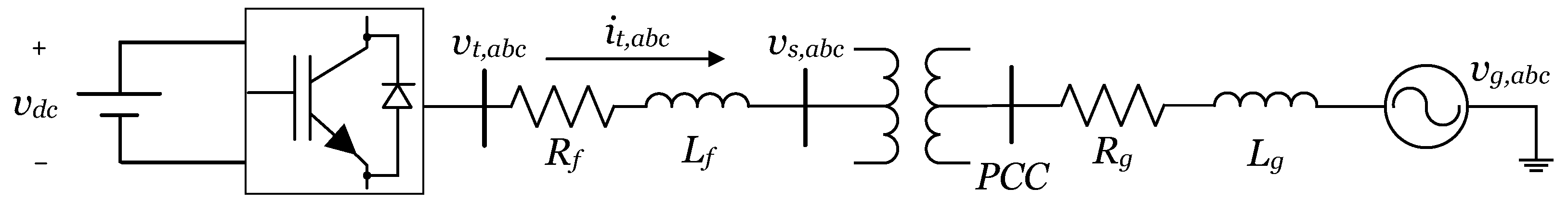
2.1. State Space Model

A single line schematic of a three-phase grid connected VSC is shown in Figure 1, in which an ideal voltage source that fixes the voltage of the DC bus is on the left, an ideal three-phase voltage source, representing the voltage of the grid, is on the right, and a step-up transformer and series RL filter are in the middle connecting the VSC to the point of common coupling (PCC). The switching harmonics of the VSC are attenuated through the use of the series filter. In the d-q frame, the state equations of the VSC are

$$\begin{array}{cc}\hfill \frac{d{i}_{t,d}}{dt}& =-\frac{R_f}{L_f}{i}_{t,d}+\omega i_{t,q}+\frac{1}{L_f}(v_{t,d}-v_{s,d})\hfill \\ \hfill \frac{d{i}_{t,q}}{dt}& =-\frac{R_f}{L_f}{i}_{t,q}-\omega i_{t,d}+\frac{1}{L_f}(v_{t,q}-v_{s,q})\hfill \end{array}$$

(1)

where $v_{t,dq}$ are the VSC output voltages, $R_f$ and $L_f$ are the resistance and inductance of the series filter, $\omega$ is the angular frequency of the system, $i_{t,dq}$ are the injected currents, and $v_{s,dq}$ are the grid voltages. Therefore, the state space representation of the VSC system is

$$\left[\begin{array}{c}\frac{d{i}_d}{dt}\\ \frac{d{i}_q}{dt}\end{array}\right]=\left[\begin{array}{cc}\frac{-R_f}{L_f}& \omega \\ -\omega & \frac{-R_f}{L_f}\end{array}\right]\left[\begin{array}{c}{i}_d\\ i_q\end{array}\right]+\left[\begin{array}{c}\frac{1}{L_f}\end{array}\right]\left[\begin{array}{c}{v}_{t,d}-v_{s,d}\\ v_{t,q}-v_{s,q}\end{array}\right]$$

(2)

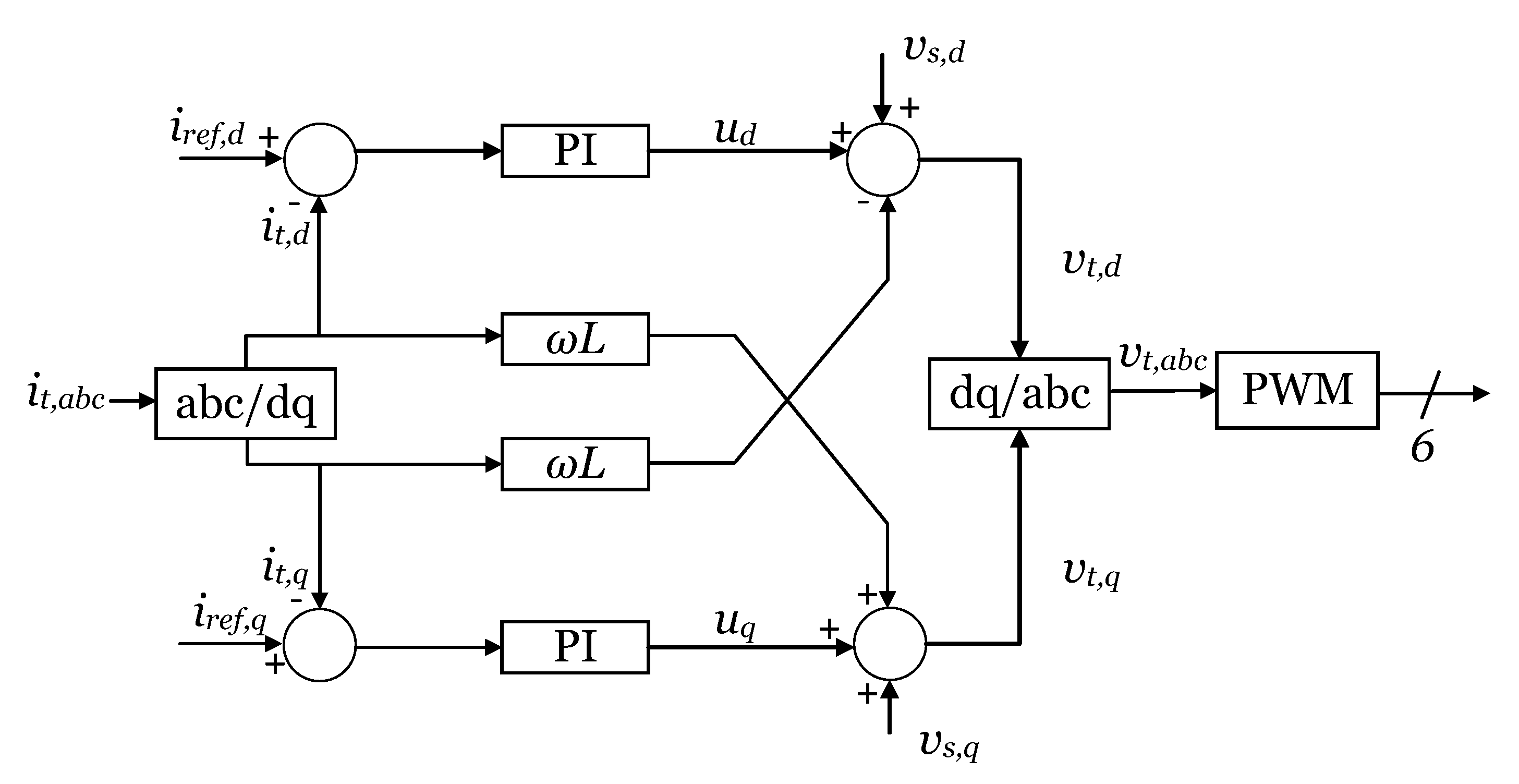
2.2. Decoupled Current Control

As shown in (1), the $\omega$ term in the dynamic model of the VSC couples the direct and quadrature axes. The axes can be decoupled by defining auxiliary variables $u_d$ & $u_q$, resulting in two decoupled first-order linear equations [4]:

$$\begin{array}{cc}\hfill u_d& =\frac{1}{L_f}(v_{t,d}+\omega L_f{i}_{t,q}-v_{s,d})\hfill \\ \hfill u_q& =\frac{1}{L_f}(v_{t,q}-\omega L_f{i}_{t,d}-v_{s,q})\hfill \end{array}$$

(3)

Substituting $u_d$ & $u_q$ in to (1) results in

$$\begin{array}{cc}\hfill \frac{d{i}_{t,d}}{dt}& =-\frac{R_f}{L_f}{i}_{t,d}+u_d\hfill \\ \hfill \frac{d{i}_{t,q}}{dt}& =-\frac{R_f}{L_f}{i}_{t,q}+u_q\hfill \end{array}$$

(4)

Therefore, the state space model becomes:

$$\left[\begin{array}{c}\frac{d{i}_d}{dt}\\ \frac{d{i}_q}{dt}\end{array}\right]=\left[\begin{array}{cc}-\frac{R}{L}& 0\\ 0& -\frac{R}{L}\end{array}\right]\left[\begin{array}{c}{i}_{t,d}\\ i_{t,q}\end{array}\right]+\frac{R}{L}\left[\begin{array}{c}{u}_d\\ u_q\end{array}\right]$$

(5)

Equation (6) shows the decoupled system’s transfer function, where $K=\frac{1}{R_f}$ and $T=\frac{L_f}{R_f}$.

$$G_s\left(s\right)=\frac{1}{R_f+s{L}_f}=\frac{K}{1+sT}$$

(6)

As seen in (4), $i_d$ & $i_q$ can be controlled using $u_d$ & $u_q$. A feedforward control structure is developed with a PI controller as the compensator in order to successfully track the current reference signals and compensate the coupling terms. PI controllers are implemented within the decoupled structure due to their ease of design and ability to quickly eliminate steady state error when there is a change in the reference [4]. Figure 2 shows the complete decoupled current control scheme of the VSC. Each current loop is independently controlling its respective terminal current ($i_{t,d}$ & $i_{t,q}$) in order to compute the desired terminal voltages ($v_{t,d}$ & $v_{t,q}$). The terminal voltages are transferred from the $dq0$-frame back to the $abc$-frame in order to generate the necessary gating signals from the pulse-width modulation (PWM).

The system experiences delays due to the PWM and computations within the control loop; these delays are represented by the transfer function in (7) [23,24]. The total time delay in the control loop is defined by $T_{eq}$, where $T_{eq}=\frac{1}{2f_{sw}}$.

$$G_{Delay}\left(s\right)=\frac{1}{1+s{T}_{eq}}$$

(7)

The transfer function of the PI controller is shown below

$$G_{PI}\left(s\right)=k_p+\frac{k_i}{s}=\frac{k_p(1+s{T}_i)}{s{T}_i}$$

(8)

where $k_p$ and $k_i$ represent the proportional and integral gains and $T_i$ is the integrator time constant. Thus, the open-loop transfer function of the decoupled current control loop is defined as

$$\begin{array}{cc}\hfill G_{OL}\left(s\right)& =G_{PI}\left(s\right)·G_{Delay}\left(s\right)·G_s\left(s\right)\hfill \\ \hfill & =\left(\frac{k_p(1+s{T}_i)}{s{T}_i}\right)\left(\frac{1}{1+s{T}_{eq}}\right)\left(\frac{K}{1+sT}\right)\hfill \end{array}$$

(9)

In order to achieve pole-zero cancellation, $k_p=\frac{L_f}{\tau }$ and $T_i=T$, where $\tau$ is a design variable ranging from 0.5 to 5 ms. This design variable determines the controller’s transient behavior as well as its response time. In practice, it is quite difficult to achieve pole-zero cancellation due to time delays caused by the PWM and inability to precisely measure the values of the $i_{dq}$, $R_f$, $L_f$, etc. In real systems this results in the axes not being fully decoupled [4,24].

3. LSTM-Based Control Technique

3.1. Motivation

References [7,25,26] show that neural network-based control, specifically RNNs can be used as a method of control for grid-connected converters such as the VSC. However, the training of RNNs are subject to training issues such as the vanishing gradient and exploding gradient problems which affect the network’s ability to understand the dynamics of the system. This paper proposes a control scheme that uses an LSTM-based controller that eliminates the need for model-based control of the VSC and offers better robustness.

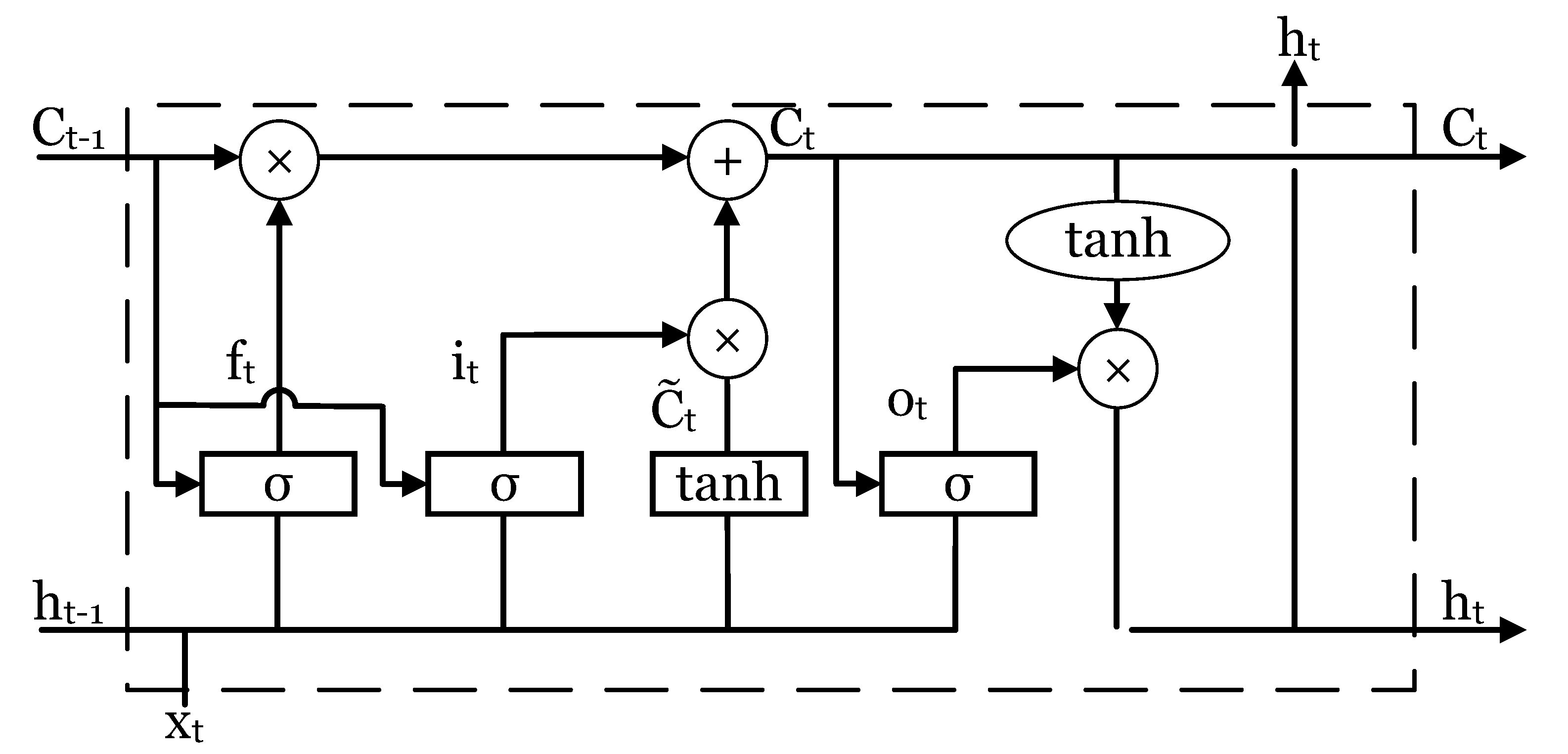
3.2. Overview of LSTM Networks

LSTM networks are comprised of multiple LSTM cells, whose inputs are the current time step input ($x_t$), previous cell state ($C_{t-1}$), and the previous network output ($h_{t-1}$). The LSTM cell controls what information is stored and removed in each cell via gate units and outputs the current cell state ($C_t$) and network output ($h_t$). Figure 3 shows the diagram of a LSTM cell and its gate units.

The LSTM network first determines what data will be disregarded from the previous cell state through its forget gate. This gate selects the values in $C_{t-1}$ through a sigmoid layer to evaluate $x_t$ and $h_{t-1}$. The sigmoid function constrains the output between 0 and 1 and its slope is continuously differentiable. If the output of the sigmoid is 0, then the value from the previous cell will not be passed to the current cell. If the value is 1, then the value will be retained. The sigmoid function is defined in (10), while the forget gate is shown in (11).

$$\sigma \left(x\right)=\frac{1}{1+e^{-x}}$$

(10)

$$f_t=\sigma (W_f·[C_{t-1},h_{t-1},x_t]+b_f)$$

(11)

The LSTM stores new data in the cell state by determining which values will be updated and the values they’ll be updated with. This is done by using the input gate which uses a sigmoid layer to select the updated values as seen in (12).

$$i_t=\sigma (W_i·[C_{t-1},h_{t-1},x_t]+b_i)$$

(12)

A hyperbolic tangent layer is used to calculate the new values that will be used to update the selected values. The hyperbolic tangent function is continuous and differentiable at all points and bounds the output between −1 and 1. Equation (13) shows the new values used to update the cell.

$$\widetilde{C_t}=tanh(W_C·[h_{t-1},x_t]+b_C)$$

(13)

The cell state is updated by multiplying the forget gate by the previous cell state and adding it to the product of (12) and (13).

$$C_t=f_t\ast C_{t-1}+i_t\ast \widetilde{C_t}$$

(14)

In order to determine the output of the cell, (15) shows the output gate using a sigmoid layer to determine which values will be outputted. The output is then determined by taking the product of the output gate and the hyperbolic tangent of the current cell state as seen in (16).

$$o_t=\sigma (W_o·[C_t,h_{t-1},x_t]+b_o)$$

(15)

$$h_t=o_t\ast tanh\left(C_t\right)$$

(16)

The gating units allow LSTM to capture the dynamics and correlation within both long and short time series data sets. This improvement of RNNs cause LSTMs to be more desirable when training on long time series datasets as they are able to resolve issues associated with long term dependencies such as the vanishing and exploding gradients.

3.3. Problem Formulation

Even though the VSC has good dynamic response under the conventional method, studies show that there are several limitations with this control method [6,7]. The conventional method requires accurate mathematical models of the VSC, which may not always be available [26]. Additionally mathematical models are developed using constant parameters. However, model parameters change under different environmental conditions. The performance of the conventional method may deteriorate due to the aforementioned issues [8,27]. Therefore, new strategies need to be proposed for a more robust performance of a grid-connected VSC.

Robust control of a grid-connected VSC can be formulated as a regression problem that can be solved using supervised learning. The objective of this method of learning is to develop models that are capable of detecting the underlying relationship between the inputs and outputs and yield accurate results on new data sets. Thus, supervised learning-based controls are capable of fitting a function that will be agnostic to the system. One method of solving supervised learning problems is through neural networks. Neural networks are universal approximators that are capable of capturing a system’s responses with very little system knowledge [28].

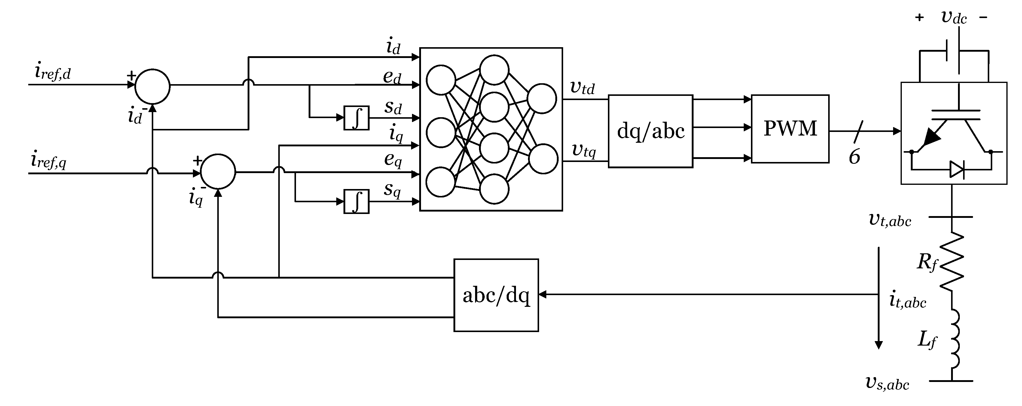
3.4. Proposed Method

The LSTM-based control architecture for a three-phase grid-connected VSC is shown in Figure 4. The controller implements a fast inner current-loop by replacing the two PI $dq$ controllers used in the conventional control approach with an LSTM-based controller. The proposed LSTM network for the VSC is a fully connected feed forward network with six inputs, two hidden layers (100 LSTM units per hidden layer), two outputs, and hyperbolic tangent activation functions at each node. The amount of hidden layers and units per layer are found via trial and error. Figure 4 shows the network’s architecture within a grid-connected VSC similar to the one shown in Figure 1. As shown in the figure, the input signals of the network are the measured currents ${\overrightarrow{i}}_{dq}\left(t\right)$, the error of the currents ${\overrightarrow{e}}_{dq}\left(t\right)$, and the integral of the error signals ${\overrightarrow{s}}_{dq}\left(t\right)$. In [25], it is noted that that the inclusion of the integral term resolves steady-state tracking error that occurs when there are parameter changes within the system, ${\overrightarrow{s}}_{dq}\left(t\right)$ is defined in (17). The network computes the outputs ${\overrightarrow{v}}_{t,dq}\left(t\right)$ at each time step.

$${\overrightarrow{s}}_{dq}\left(t\right)={\int }_0^{T_s}{\overrightarrow{e}}_{dq}\left(t\right)dt={\int }_0^{T_s}\left({\overrightarrow{i}}_{dq,ref}\left(t\right)-{\overrightarrow{i}}_{dq}\left(t\right)\right)dt$$

(17)

The system is controlled using only a decoupled current control method for the grid-connected VSC. In this method, the controller is designed to follow current set points and does so under any condition as long as it is stable. For example, if a fault occurs at the inverter terminals, the current goes through a short transient before settling back at its set point. It should be noted that if an outer loop is used to control power, the controller performs differently under faults. This is because the inverter cannot inject real power with the voltage reduced. Therefore, it increases the active current until it reaches its upper limit.

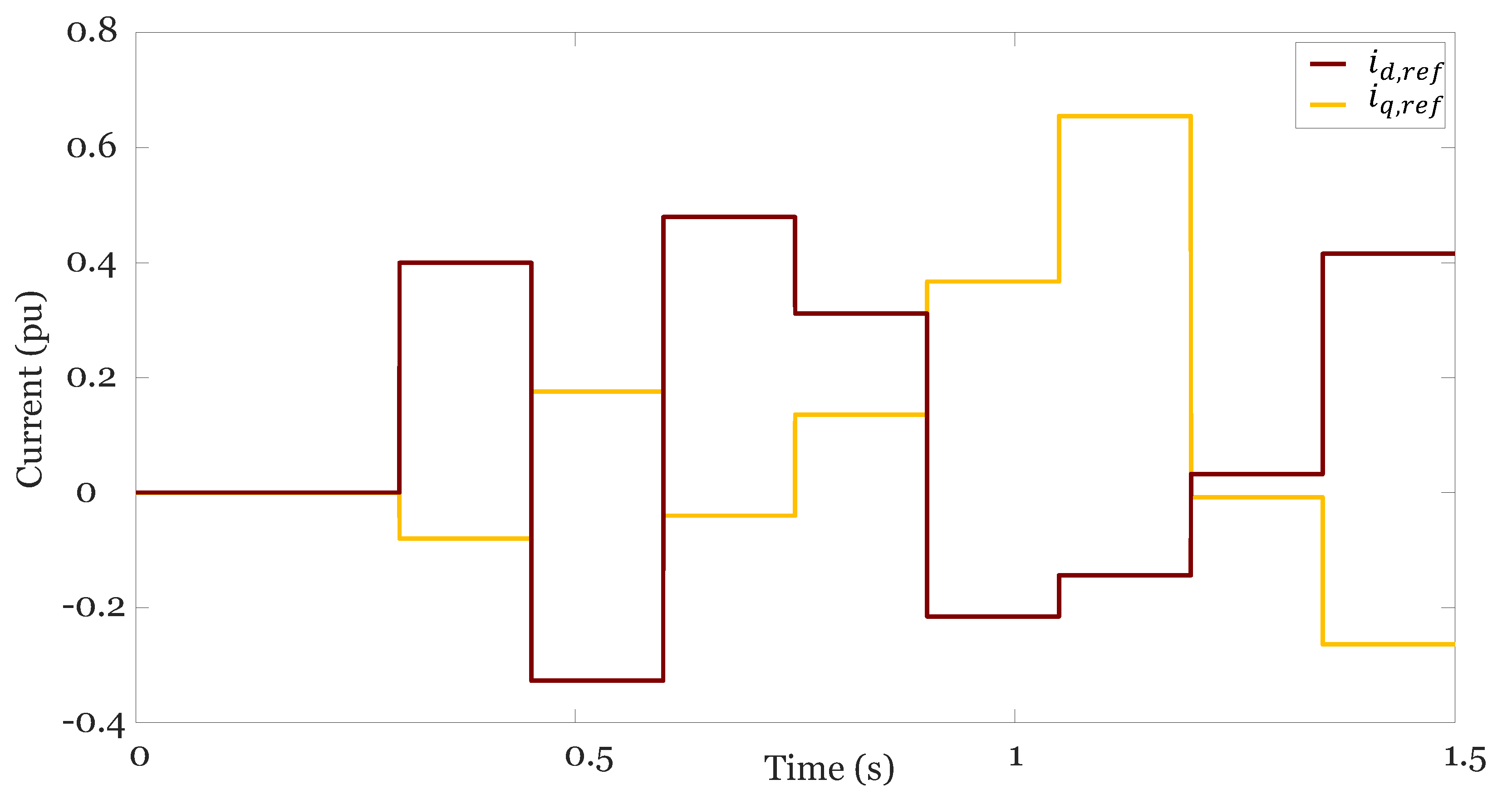
3.5. Gathering of Training Data

The training data for the LSTM-based controller is generated by performing set point changes in both the direct and quadrature axes of well tuned conventional controlled models of a grid-connected VSC in Simulink. The parameters of the VSC model are shown in

Table 1. System Parameters.

Parameter	Value
DC bus voltage	$V_{dc}=750$ V
Grid voltage (RMS)	$V_g=420$ V
Filter Resistance	$R_f=1$$\mathsf{\Omega }$
Filter inductance	$L_f=8$ mH
Switching frequency	$f_{sw}=20$ kHz
Grid Resistance	$R_s=25\mathrm{m}\mathsf{\Omega }$
Grid Inductance	$L_s=45\mathsf{\mu }\mathrm{H}$

. The values for the set point changes were randomly selected from a range of values that did not exceed the rated current limit or caused the voltage to reach saturation. Thus, the training data set for the network is comprised of the good training data that will not cause the network to be improperly trained. The use of finely tuned decoupled current controllers to generate the training data allow the LSTM-based controller to learn how to control each current component independently. Figure 5 shows an example of these set point changes, where the reference values would be changed after every 0.15 s starting at 0.3 s. The total duration of each simulation is for 1.5 s while the sampling time for the system is chosen as $T_s$ = 0.025 ms. In order to avoid input saturation and improve the accuracy of the network, the inputs are feature scaled using min-max scaling (18). Feature scaling reduces the impact of certain features and gives equal importance to each feature.

$$x^{\prime }=\frac{x-x_{min}}{x_{max}-x_{min}}$$

(18)

The proposed LSTM model, as shown in Figure 4, is built and trained in Python using the Keras and TensorFlow libraries. The model is compiled using the Adam optimizer, MSE loss function, and a learning rate of 0.01. The MSE loss function calculates the average of the squared difference between the observed and targeted values. The MSE loss function is shown in (18), where $y_i$ is the observed value and ${\tilde{y}}_i$ represents the target value.

$$\mathrm{MSE}=\frac{1}{n}\sum _{i=1}^n{(y_i-{\tilde{y}}_i)}^2$$

(19)

The data set is split into two parts, 80% for training data and 20% for testing data. This is done to ensure that there is enough training data to train the model. Once the data is properly feature scaled and split, the training data is fed into the LSTM network and the model begins training. The model is trained offline using batch training. The model is trained for 400 epochs and its loss curve is shown in Figure 6.

4. Performance Evaluation

A simulation system of a grid-connected VSC is built in Simulink in order to evaluate the performance of the LSTM-based controller with the conventional controller. Four case studies for which the model is not trained for are discussed below. Figure 7 shows the Simulink model of the grid-connected VSC.

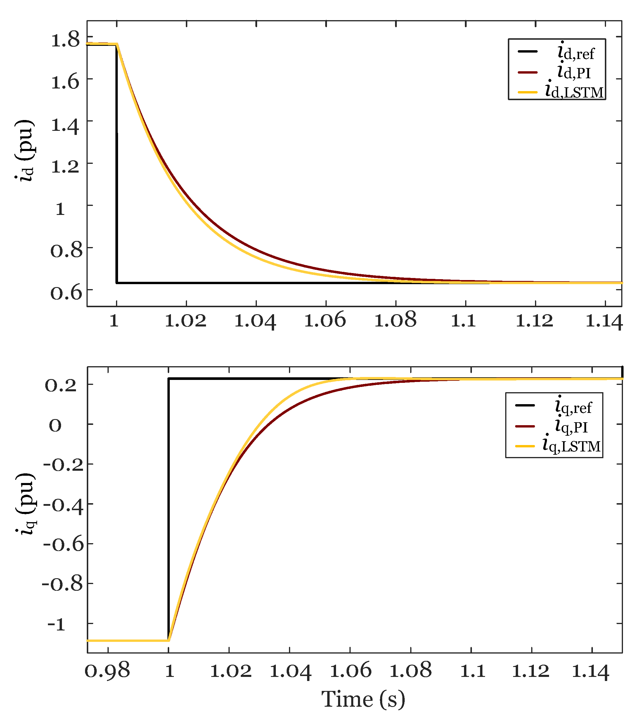
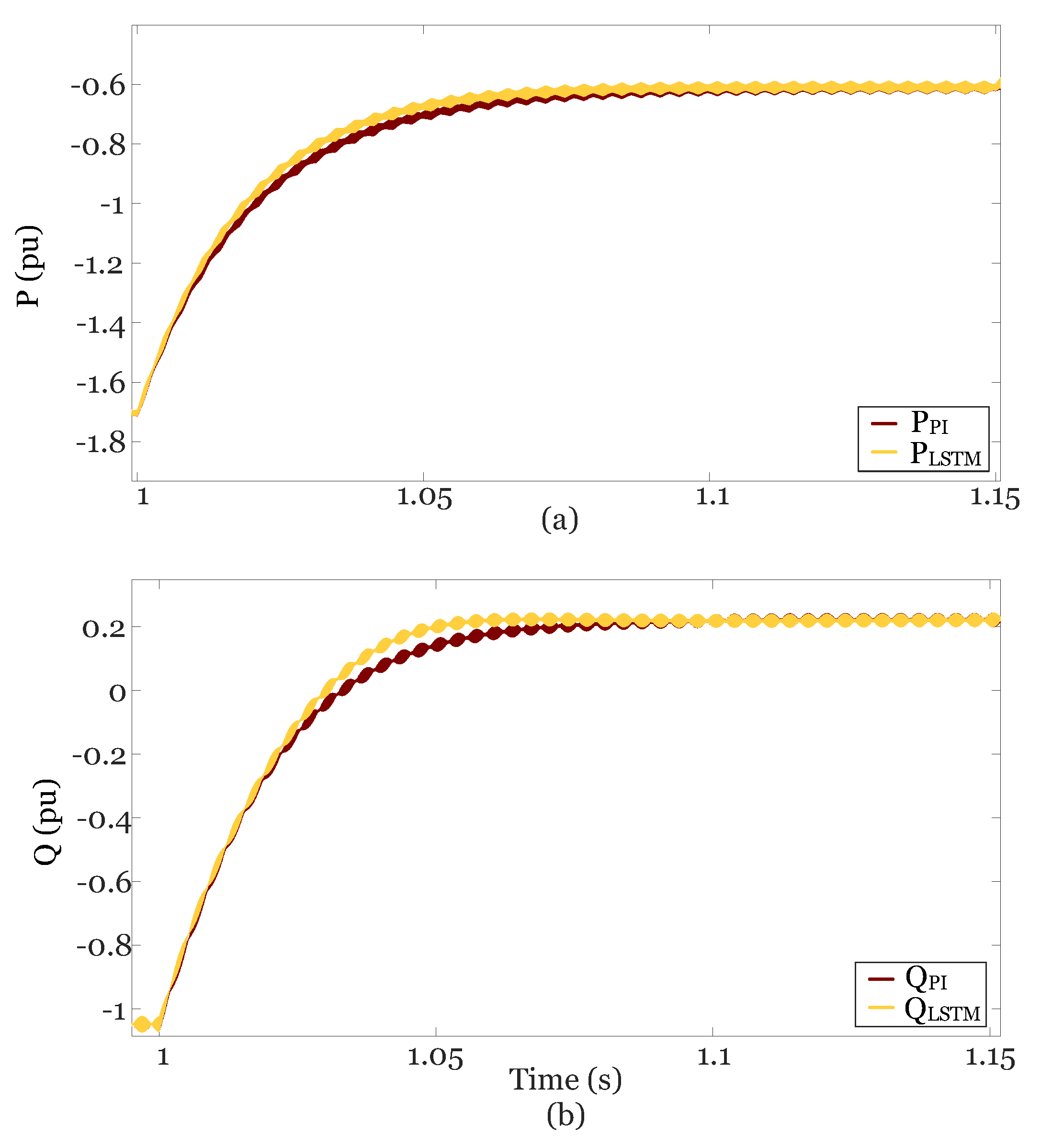
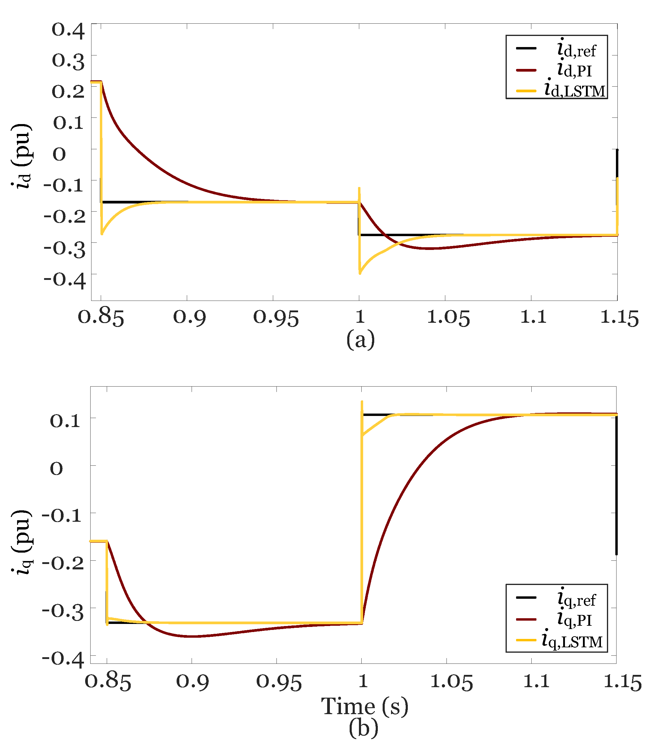
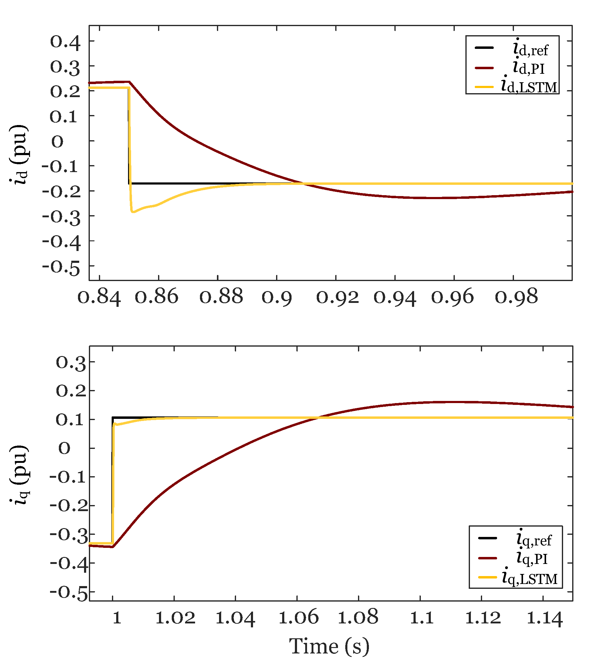
4.1. Step Change in Direct and Quadratic Current Reference

A step change from 1.76 pu to 0.63 pu in $i_{d,ref}$ occurs at t = 1 s. Figure 8a shows that the LSTM-based controller successfully tracking $i_d$ during a step change. The LSTM has a settling time of 0.09 s while the conventional controller settles in 0.12 s.

$i_{q,ref}$ changes from −1.09 pu to 0.23 pu at t = 1 s in Figure 8b. The LSTM has a settling time of 0.06 s while the conventional controller settles in 0.11 s, demonstrating the successful tracking of $i_q$ during a step change in $i_{q,ref}$. Figure 9 shows the real and reactive power response to the step changes shown in Figure 8.

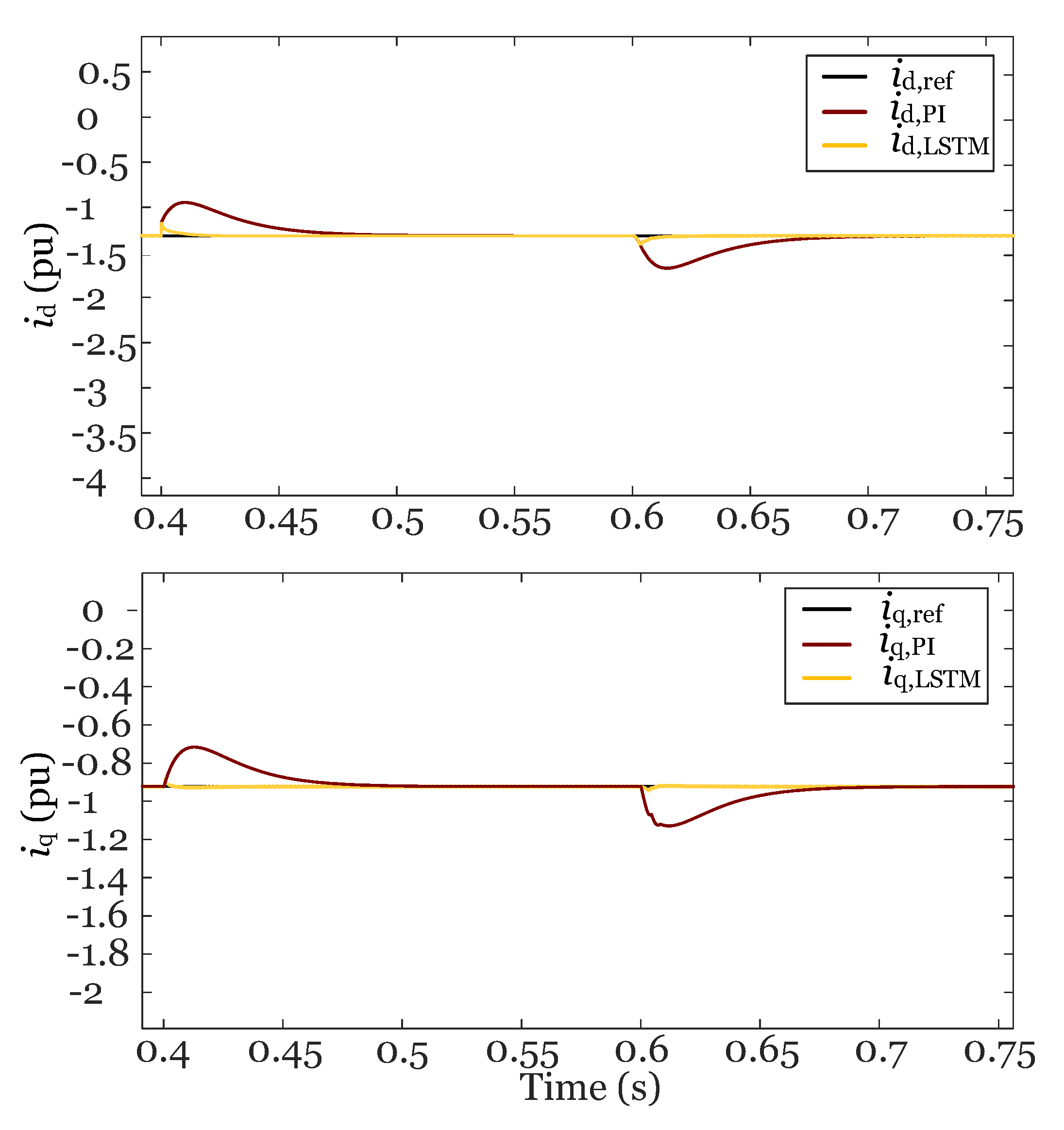
4.2. Fault Analysis at PCC

Figure 10, Figure 11, Figure 12 and Figure 13 show the responses for different simulated faults that occur at t = 0.4 s and lasts for 10 cycles at the PCC. Figure 10 shows the response for a three-phase fault, Figure 11 shows the response for a single-phase fault (A-G), Figure 12 for a phase-phase fault (A-B), and Figure 13 shows the response for a double phase-ground fault (B-C-G). As seen in the figures, the LSTM-based controller is able to reduce the overshoot and undershoot that occurs during a fault as well as maintain stability once the fault is cleared; performing significantly better than the conventional controller.

4.3. Decreasing SCR

The SCR of the system is decreased causing the system to be poorly connected to the grid. In Figure 14a, $i_{d,ref}$ changes from −0.17 pu to −0.297 pu at t = 1.3 s. The LSTM has a settling time of 0.02 s while the conventional controller settles in 0.07 s. In Figure 14b, $i_{q,ref}$ changes from −0.02 pu to −0.17 pu at t = 0.55 s. The LSTM has a settling time of 0.02 s while the conventional controller settles in 0.07 s, demonstrating the effectiveness of the controller even under weak grid connection. Figure 15 shows the real and reactive power response to the step changes shown in Figure 14.

4.4. Changing the Grid Filter

The inductance of the grid filter is reduced by 20%. In Figure 16a, $i_{d,ref}$ changes from 0.21 pu to −0.17 pu at t = 0.85 s and from −0.17 pu to −0.27 pu at t = 1 s. In Figure 16b, $i_{q,ref}$ changes from −0.16 pu to −0.33 pu at t = 0.85 s and from −0.33 pu to 0.11 pu at t = 1 s. The LSTM-based controller settles faster than the conventional controller demonstrating the superiorty of the proposed method under parameter changes. Figure 17 shows the real and reactive power response to the step changes shown in Figure 16.

The inductance of the grid filter is increased by 50%. In Figure 18a, $i_{d,ref}$ changes from 0.21 pu to −0.17 pu at t = 0.85 s. The LSTM has a settling time of 0.05 s while the conventional controller is unable to successfully track the set point change. In Figure 18b, $i_{q,ref}$ changes from −0.33 pu to −0.11 pu at t = 1 s. The LSTM has a settling time of 0.04 s while the conventional controller is unable to successfully track the set point change. The LSTM-based controller is able to operate properly when the conventional controller is not, demonstrating the robustness of the controller to system paramter changes.

5. Conclusions

This paper proposes an LSTM-based control scheme for grid-connected VSCs. The LSTM-based controller is trained in Python using the Keras and TensorFlow libraries. Using Simulink, a simulation system is built to test various scenarios in order to evaluate the performance of the proposed method. The LSTM-based controller outperforms the conventional control method under all cases, confirming the robustness and accuracy of the proposed method.

References

1. Davari, M.; Mohamed, Y.A.R.I. Robust Vector Control of a Very Weak-Grid-Connected Voltage-Source Converter Considering the Phase-Locked Loop Dynamics. IEEE Trans. Power Electron. 2017, 32, 977–994. [Google Scholar] [CrossRef]
2. Kazem Bakhshizadeh, M.; Wang, X.; Blaabjerg, F.; Hjerrild, J.; Kocewiak, L.; Bak, C.L.; Hesselbæk, B. Couplings in Phase Domain Impedance Modeling of Grid-Connected Converters. IEEE Trans. Power Electron. 2016, 31, 6792–6796. [Google Scholar] [CrossRef]
3. Zhou, S.; Zou, X.; Zhu, D.; Tong, L.; Zhao, Y.; Kang, Y.; Yuan, X. An Improved Design of Current Controller for LCL-Type Grid-Connected Converter to Reduce Negative Effect of PLL in Weak Grid. IEEE J. Emerg. Sel. Top. Power Electron. 2018, 6, 648–663. [Google Scholar] [CrossRef]
4. Yazdani, A.; Iravani, R. Electronic Power Conversion. In Voltage-Sourced Converters in Power Systems: Modeling, Control, and Applications; Wiley: Hoboken, NJ, USA, 2010; pp. 1–20. [Google Scholar] [CrossRef]
5. Kaura, V.; Blasko, V. Operation of a voltage source converter at increased utility voltage. IEEE Trans. Power Electron. 1997, 12, 132–137. [Google Scholar] [CrossRef]
6. Zhao, S.; Blaabjerg, F.; Wang, H. An Overview of Artificial Intelligence Applications for Power Electronics. IEEE Trans. Power Electron. 2021, 36, 4633–4658. [Google Scholar] [CrossRef]
7. Fu, X.; Li, S.; Fairbank, M.; Wunsch, D.C.; Alonso, E. Training Recurrent Neural Networks With the Levenberg–Marquardt Algorithm for Optimal Control of a Grid-Connected Converter. IEEE Trans. Neural Netw. Learn. Syst. 2015, 26, 1900–1912. [Google Scholar] [CrossRef] [Green Version]
8. Olivares, D.E.; Mehrizi-Sani, A.; Etemadi, A.H.; Cañizares, C.A.; Iravani, R.; Kazerani, M.; Hajimiragha, A.H.; Gomis-Bellmunt, O.; Saeedifard, M.; Palma-Behnke, R.; et al. Trends in Microgrid Control. IEEE Trans. Smart Grid 2014, 5, 1905–1919. [Google Scholar] [CrossRef]
9. Bose, B.K. Neural Network Applications in Power Electronics and Motor Drives—An Introduction and Perspective. IEEE Trans. Ind. Electron. 2007, 54, 14–33. [Google Scholar] [CrossRef]
10. Meireles, M.; Almeida, P.; Simoes, M. A comprehensive review for industrial applicability of artificial neural networks. IEEE Trans. Ind. Electron. 2003, 50, 585–601. [Google Scholar] [CrossRef]
11. Sun, Y.; Li, S.; Lin, B.; Fu, X.; Ramezani, M.; Jaithwa, I. Artificial Neural Network for Control and Grid Integration of Residential Solar Photovoltaic Systems. IEEE Trans. Sustain. Energy 2017, 8, 1484–1495. [Google Scholar] [CrossRef]
12. Hochreiter, S.; Schmidhuber, J. Long Short-term Memory. Neural Comput. 1997, 9, 1735–1780. [Google Scholar] [CrossRef] [PubMed]
13. Che, Z.; Purushotham, S.; Cho, K.; Sontag, D.; Liu, Y. Recurrent Neural Networks for Multivariate Time Series with Missing Values. Sci. Rep. 2018, 8, 6085. [Google Scholar] [CrossRef] [PubMed] [Green Version]
14. Sutskever, I.; Vinyals, O.; Le, Q.V. Sequence to Sequence Learning with Neural Networks. arXiv 2014, arXiv:1409.3215. [Google Scholar]
15. Gers, F.; Schmidhuber, J.; Cummins, F. Learning to Forget: Continual prediction with LSTM. Neural Comput. 2000, 12, 2451–2471. [Google Scholar] [CrossRef]
16. Greff, K.; Srivastava, R.K.; Koutnik, J.; Steunebrink, B.R.; Schmidhuber, J. LSTM: A Search Space Odyssey. IEEE Trans. Neural Netw. Learn. Syst. 2017, 28, 2222–2232. [Google Scholar] [CrossRef] [PubMed] [Green Version]
17. Alazab, M.; Khan, S.; Krishnan, S.S.R.; Pham, Q.V.; Reddy, M.P.K.; Gadekallu, T.R. A Multidirectional LSTM Model for Predicting the Stability of a Smart Grid. IEEE Access 2020, 8, 85454–85463. [Google Scholar] [CrossRef]
18. Farsi, B.; Amayri, M.; Bouguila, N.; Eicker, U. On Short-Term Load Forecasting Using Machine Learning Techniques and a Novel Parallel Deep LSTM-CNN Approach. IEEE Access 2021, 9, 31191–31212. [Google Scholar] [CrossRef]
19. Wen, S.; Wang, Y.; Tang, Y.; Xu, Y.; Li, P.; Zhao, T. Real-Time Identification of Power Fluctuations Based on LSTM Recurrent Neural Network: A Case Study on Singapore Power System. IEEE Trans. Ind. Inform. 2019, 15, 5266–5275. [Google Scholar] [CrossRef]
20. Xie, J.; Sun, W. A Transfer and Deep Learning-Based Method for Online Frequency Stability Assessment and Control. IEEE Access 2021, 9, 75712–75721. [Google Scholar] [CrossRef]
21. Liu, L.; Fei, J.; An, C. Adaptive Sliding Mode Long Short-Term Memory Fuzzy Neural Control for Harmonic Suppression. IEEE Access 2021, 9, 69724–69734. [Google Scholar] [CrossRef]
22. Yang, Y.; Smith, D.; Rajasegaran, J.; Seneviratne, S. Power Control for Body Area Networks: Accurate Channel Prediction by Lightweight Deep Learning. IEEE Internet Things J. 2021, 8, 3567–3575. [Google Scholar] [CrossRef]
23. Sangwongwanich, A.; Abdelhakim, A.; Yang, Y.; Zhou, K. Control of single-phase and three-phase DC/AC converters. In Control of Power Electronic Converters and Systems; Academic Press: Cambridge, MA, USA, 2018; pp. 153–173. [Google Scholar] [CrossRef]
24. Yazdanian, M.; Mehrizi-Sani, A. Internal Model-Based Current Control of the RL Filter-Based Voltage-Sourced Converter. IEEE Trans. Energy Convers. 2014, 29, 873–881. [Google Scholar] [CrossRef]
25. Li, S.; Fairbank, M.; Johnson, C.; Wunsch, D.C.; Alonso, E.; Proao, J.L. Artificial Neural Networks for Control of a Grid-Connected Rectifier/Inverter Under Disturbance, Dynamic and Power Converter Switching Conditions. IEEE Trans. Neural Netw. Learn. Syst. 2014, 25, 738–750. [Google Scholar] [CrossRef] [PubMed] [Green Version]
26. Fu, X.; Li, S.; Jaithwa, I. Implement Optimal Vector Control for LCL-Filter-Based Grid-Connected Converters by Using Recurrent Neural Networks. IEEE Trans. Ind. Electron. 2015, 62, 4443–4454. [Google Scholar] [CrossRef]
27. Luo, A.; Tang, C.; Shuai, Z.; Tang, J.; Xu, X.Y.; Chen, D. Fuzzy-PI-Based Direct-Output-Voltage Control Strategy for the STATCOM Used in Utility Distribution Systems. IEEE Trans. Ind. Electron. 2009, 56, 2401–2411. [Google Scholar] [CrossRef]
28. Hornik, K.; Stinchcombe, M.; White, H. Multilayer feedforward networks are universal approximators. Neural Netw. 1989, 2, 359–366. [Google Scholar] [CrossRef]
Figure 1. Single line representation of three-phase grid-connected VSC.
Energies 16 00453 g001
Figure 2. Conventional dq current control structure.
Energies 16 00453 g002
Figure 3. LSTM cell structure.
Energies 16 00453 g003
Figure 4. LSTM control structure for grid-connected VSC.
Energies 16 00453 g004
Figure 5. Example training data for LSTM network.
Energies 16 00453 g005
Figure 6. Loss curve for LSTM network.
Energies 16 00453 g006
Figure 7. Simulink model of three-phase grid-connected VSC.
Energies 16 00453 g007
Figure 8. Controller response to step changes in i d , r e f and i q , r e f . (a) i d , r e f change; (b) i q , r e f change.
Energies 16 00453 g008
Figure 9. Real and reactive power response to step changes in i d , r e f and i q , r e f . (a) Real power; (b) Reactive power.
Energies 16 00453 g009
Figure 10. Controller response to a three-phase fault at PCC.
Energies 16 00453 g010
Figure 11. Controller response to a single phase-ground fault at PCC.
Energies 16 00453 g011
Figure 12. Controller response to a phase-phase fault at PCC.
Energies 16 00453 g012
Figure 13. Controller response to a double phase-ground fault at PCC.
Energies 16 00453 g013
Figure 14. Controller response for a lower SCR. (a) i d , r e f change; (b) i q , r e f change.
Energies 16 00453 g014
Figure 15. Real and reactive power response for a lower SCR. (a) Real power; (b) Reactive power.
Energies 16 00453 g015
Figure 16. Controller response to 20% decrease in the inductance of the grid filter. (a) i d , r e f change; (b) i q , r e f change.
Energies 16 00453 g016
Figure 17. Real and reactive power response 20% decrease in the inductance of the grid filter. (a) Real power; (b) Reactive power.
Energies 16 00453 g017
Figure 18. Controller response to 50% increase in the inductance of the grid filter. (a) i d , r e f change; (b) i q , r e f change.
Energies 16 00453 g018