Harmonic Contribution Assessment Based on the Random Sample Consensus and Recursive Least Square Methods

Abstract

This paper deals with a method of quantifying the harmonic contribution of each harmonic source to system voltage distortion. Assessing the harmonic contribution of individual harmonic sources is essential for mitigating and managing system harmonic levels. Harmonic contributions can be evaluated using the principle of voltage superposition with equivalent voltage models for harmonic sources. In general, the parameters of equivalent voltage models are estimated numerically because it is difficult to measure them directly. In this paper, we present an effective method for estimating equivalent model parameters based on the random sample consensus (RANSAC) and recursive least square (RLS) with a variable forgetting factor. The procedure for quantifying harmonic contributions using equivalent models is also introduced. Additionally, we propose a network diagram of harmonic contributions that makes it easy to understand the harmonic distortion contributions of all harmonic sources.

1. Introduction

Harmonic distortion, which appears as a deviation from the nominal sine wave of AC voltage and current, is one of the major power quality problems in power systems. As harmonic distortion becomes more severe, various problems such as energy losses, equipment malfunctions, neutral current increase, and metering errors occur. The continued increase in non-linear loads and inverter-based renewable energy will further exacerbate harmonic pollution in power systems [1,2,3,4,5]. The effective management and mitigation of system harmonic levels require identifying the harmonic sources causing severe system voltage distortions. The traditional total harmonic distortion (THD) and total demand distortion (TDD) harmonic distortion factors only show the overall degree of harmonic distortion at a measurement point. However, they do not identify the contribution of individual harmonic sources to the system’s voltage distortions. Accordingly, several methods have been studied to quantitatively evaluate the contributions of harmonic sources to harmonic voltage distortion at a specific point [6]. In most methods, harmonic contribution assessment requires equivalent voltage models for all harmonic sources. However, since we cannot directly measure equivalent voltage model parameters, numerical approaches are used to estimate them. In [7,8,9,10,11,12,13,14], linear regression methods to estimate equivalent voltage model parameters were introduced. However, because these methods assume that harmonic sources’ equivalent voltages and impedances are constant, large errors in estimating harmonic contribution can occur with the variation in system operating conditions. Therefore, applying these methods to real systems is difficult. Other methods based on the recursive least square (RLS) algorithm, which can estimate time-varying parameters according to changes in harmonic sources, were also proposed [15,16]. However, they use constant-forgetting factors, causing potential covariance ‘wind-up’ problems and making it difficult to expect reliable estimates. To address this issue, Park et al. [17] proposed a new estimation method based on the parameter’s change detection scheme and RLS algorithm with a variable-forgetting factor. However, since all existing methods estimate parameters using measurement data, the following fundamental problem arises: estimation performance significantly degrades with the presence of outliers in measurement data. Outliers may be recorded for various reasons, causing large estimation errors even in advanced algorithms. Therefore, to improve parameter estimation performance, an effective method for removing outliers from measurement data is also required. Statistical techniques, such as data smoothing and average filtering for removing outliers, were presented [18,19,20,21]. However, they are ineffective because the average value is significantly influenced by outliers, especially when measurement data are insufficient and the equivalent parameters of harmonic sources frequently change. There is another method called the random sample consensus (RANSAC) algorithm. Basically, it determines an optimal linear model for all data and then removes outlying data not included within a certain threshold range for the linear model [22]. This algorithm is independent of changes in the measured data’s average value and is effective even when the dataset is relatively small. In this paper, we propose an advanced method based on the RANSAC and RLS algorithms to evaluate harmonic contributions. The proposed method demonstrates excellent performance when outliers exist in measurement data and even with the variation in harmonic equivalent parameters. Additionally, we developed a method of creating a harmonic contribution diagram that can intuitively understand the voltage distortion contribution of individual harmonic sources. In the case study, the proposed methods were verified through a comparative analysis of various cases.

2. Parameter Estimation of the Harmonic Source’s Equivalent Model

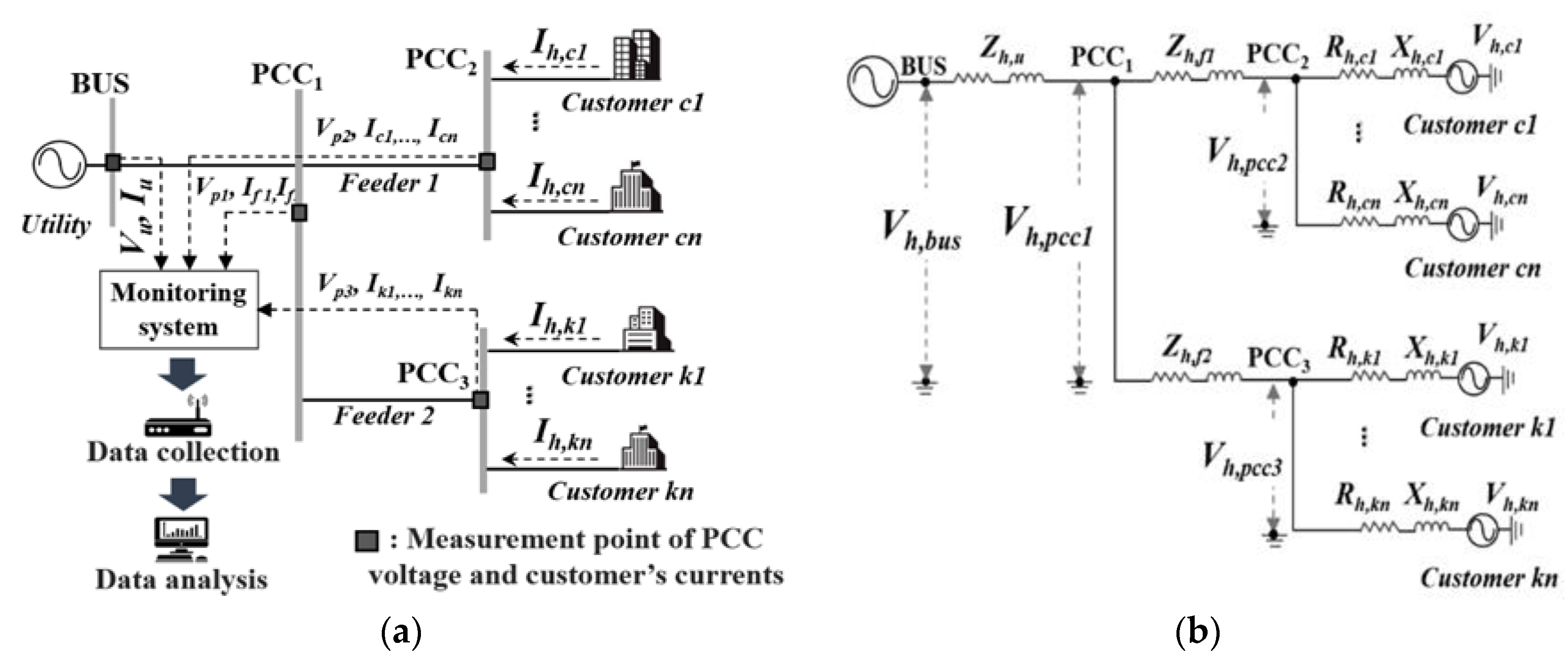
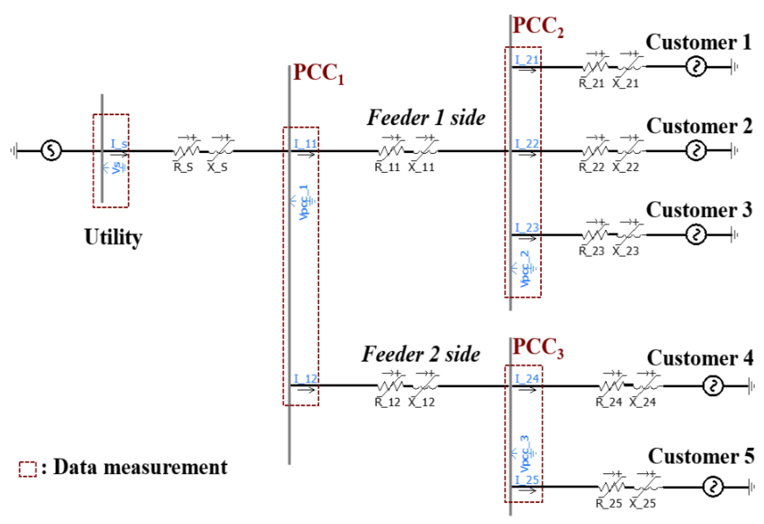
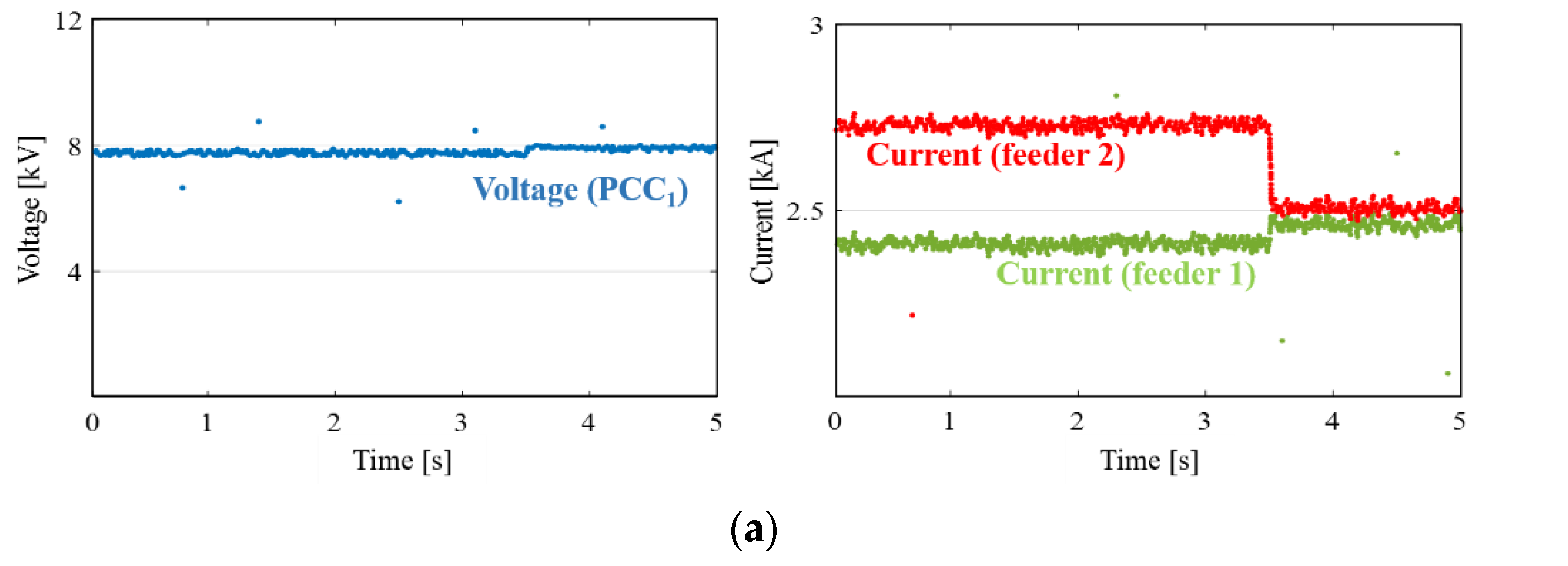
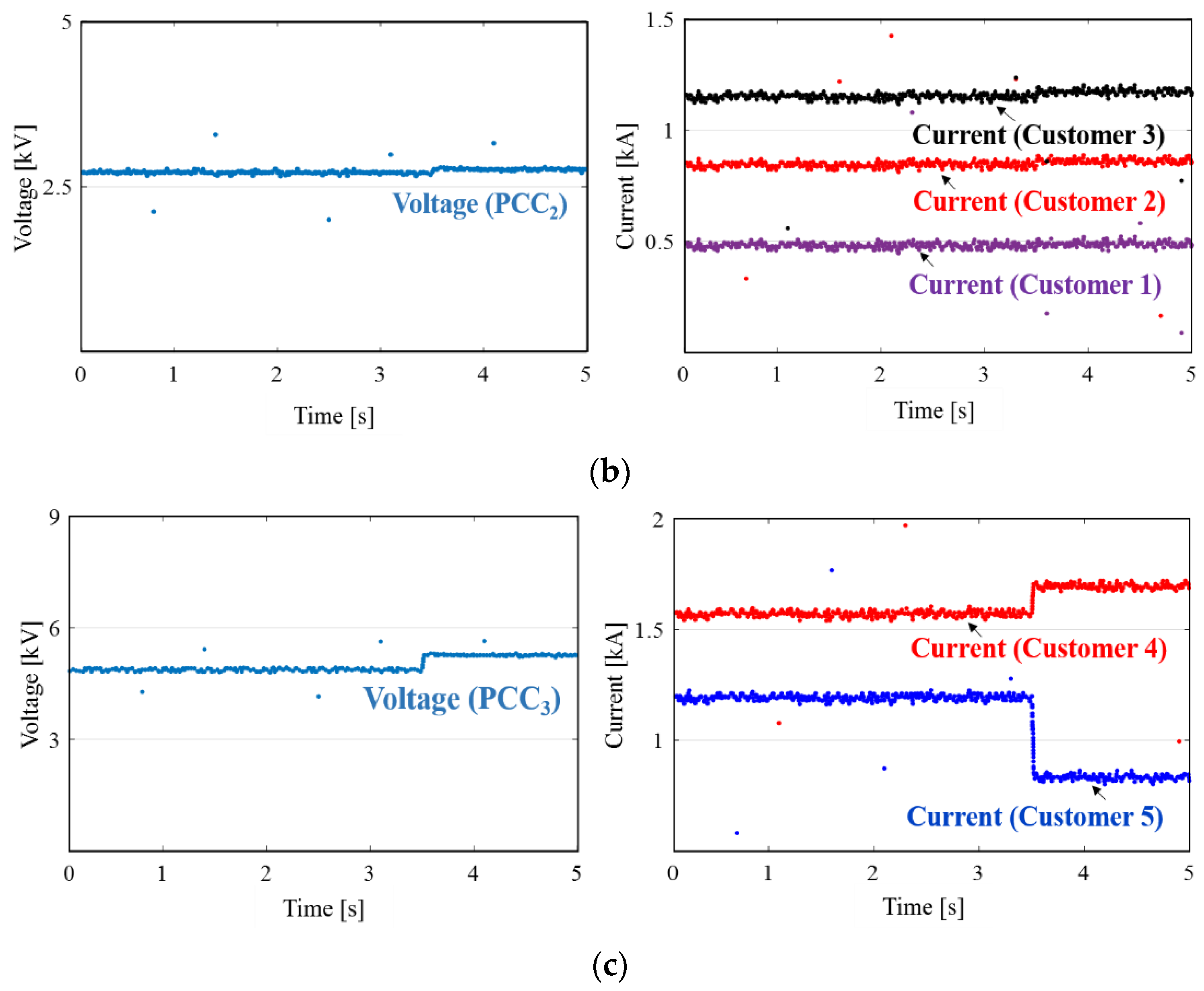
2.1. Data Measurement and the Equivalent Model Estimation of Harmonic Sources

The harmonic contribution assessment is a technique that quantitatively indicates the voltage distortion levels due to harmonic sources at the point of common coupling (PCC) in the system. For the assessment, an equivalent voltage model for harmonic sources connected to the PCC is required. The time-varying parameters of the equivalent model can be estimated using measured data at PCCs’ and numerical analysis. In this paper, an effective RLS-based method for estimating equivalent model parameters is proposed. The RLS method is an adaptive filter algorithm that is widely used for the estimation of time-varying parameter.

Figure 1 shows a typical distribution network consisting of three PCCs with harmonic sources. As shown in Figure 1a, the monitoring system measures the customers’ voltages and currents at each PCC. Figure 1b shows the equivalent model composed of impedance and voltage for the harmonic sources connected to PCCs. The equivalent model’s parameters are estimated using data measured at each PCC and the RLS method. We can express the PCC voltage as a linear equation:

$$V_{h, pcc, r}+j{V}_{h, pcc, i}=\left(R_{h,c}+j{X}_{h, c}\right)\left(I_{h, c, r}+j{I}_{h,c, i}\right)+V_{h, c, r}+j{V}_{h,c, i}$$

(1)

where R_h,c and X_h,c are the equivalent resistance and reactance of customer c for the hth harmonic order, respectively. V_h,c,r and V_h,c,i are the real and imaginary parts of the equivalent voltage of customer c for the hth harmonic order. In addition, V_h,pcc,r and V_h,pcc,i are the real and imaginary parts of PCC voltage for the hth harmonic order.

To apply the RLS algorithm for estimating the equivalent model parameters, Equation (1) is expressed in matrix form as follows:

$$Y\left(t\right)=A\left(t\right)\mathsf{\Theta }$$

(2)

$$Y\left(t\right)=\left[V_{h,pcc,r} V_{h,pcc,i}\right]$$

(3)

$$A\left(t\right)=\left[I_{h,c,r} I_{h,c,i } 1\right]$$

(4)

$$\mathsf{\Theta }=\left[\begin{array}{cc}{R}_{h,c}& X_{h,c}\\ -X_{h,c}& R_{h,c}\\ V_{h,c,r}& V_{h,c,i}\end{array}\right]$$

(5)

where $Y\left(t\right)$ and $A\left(t\right)$ are measured voltages and currents at a PCC, and $\mathsf{\Theta }$ represents the unknown parameters of the equivalent harmonic source model.

In this paper, we utilized the variable-forgetting factor RLS algorithm proposed in [17] to estimate the unknown parameter matrix $\mathsf{\Theta }$. Additionally, to improve parameter estimation performance, the parameter-change detection scheme was applied to the RLS procedure. The proposed method’s scheme adjusts the reflection of past and present data by calculating the PCC voltage’s change rate, which is calculated using Equation (6). When this value exceeds a certain threshold voltage, the RLS method is initialized to perform a new estimation. Therefore, it is possible to prevent estimation performance degradation due to past data.

$$\Delta V_{pcc}=\left|\frac{ V_{pcc}^{start}-V_{pcc}^{\left(N\right) } }{V_{pcc}^{start}}\right|\times 100\left(\%\right)$$

(6)

where $\Delta V_{pcc}$ is the PCC voltage’s change rate. $V_{pcc}^{start}$ is its starting value, which is a reference voltage for parameter-change detection. $V_{pcc}^{\left(N\right)}$ is the Nth value of the PCC voltage.

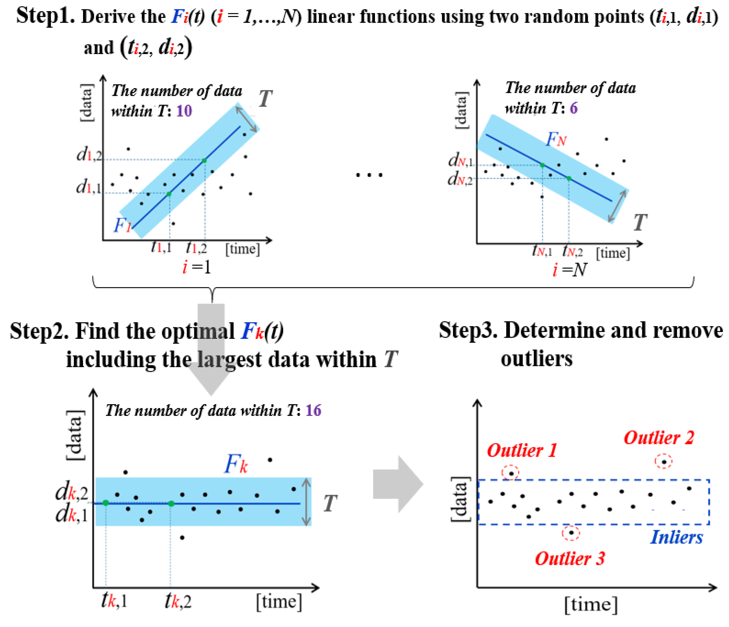
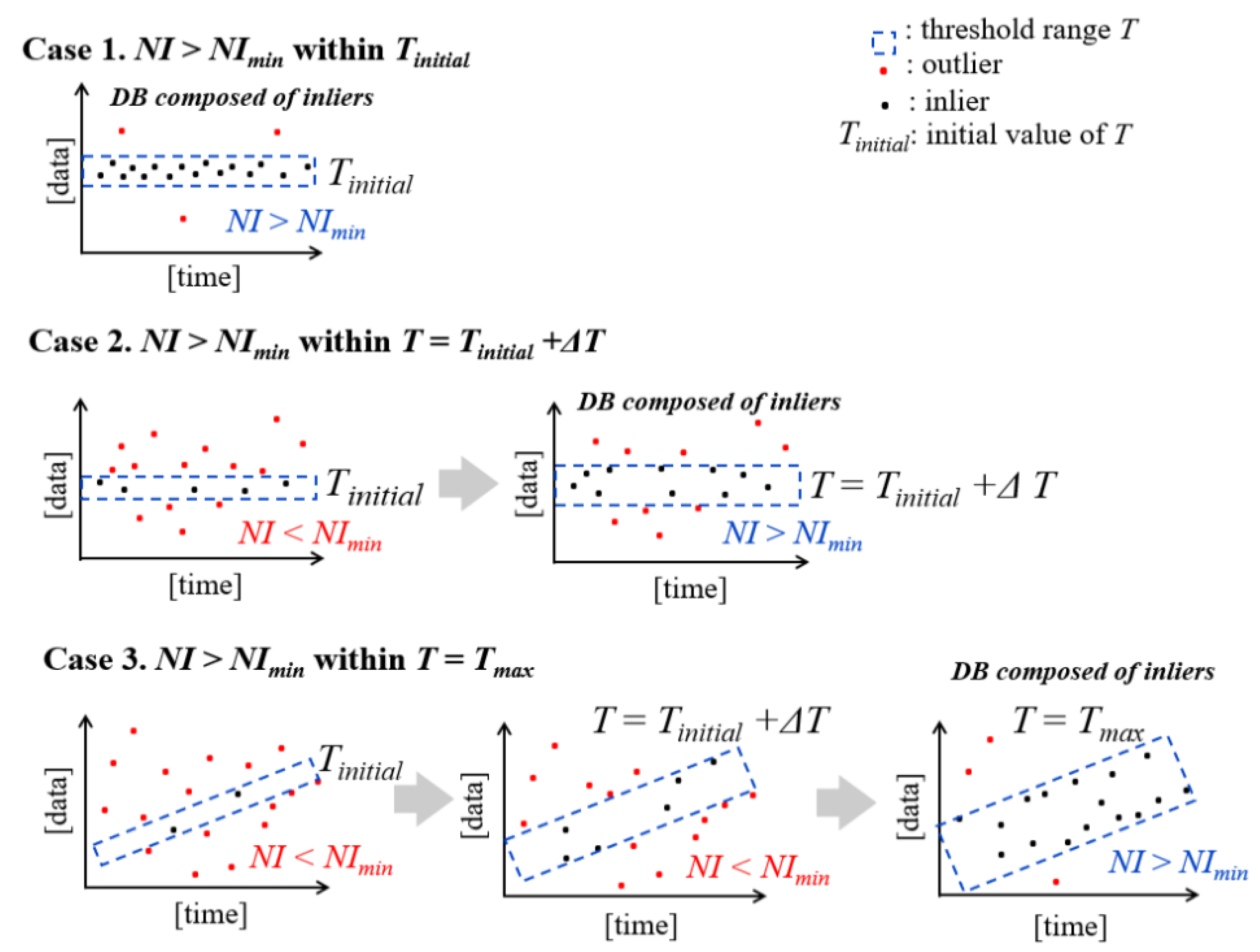
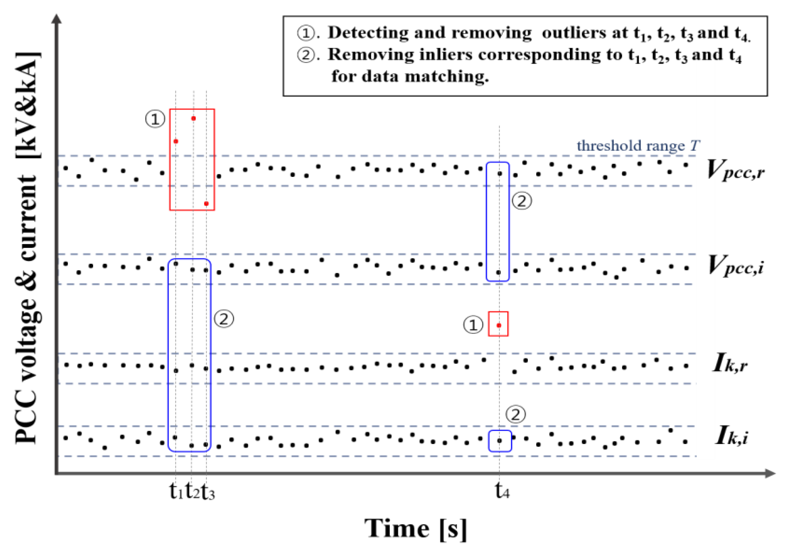
2.2. Outlier Detection and Removal Using the RANSAC Algorithm

Recently, the use of measurement devices, such as PMU, AMI, and smart meters, has been expanding, making it possible to acquire measurement data at a system’s various locations [23]. However, measurement data may include outliers due to various causes such as communication errors, power outages, and sensor malfunctions [24,25,26,27]. An outlier is a value that deviates significantly from the normal distribution of the measurement data. In applying the RLS method, there is a fundamental problem, namely the significant degradation in the parameter estimation performance in the presence of outliers in the measurement data. Therefore, to improve the performance of the RLS estimation, outliers should be detected and removed from the measured voltages and currents. In this paper, we propose an efficient RANSAC algorithm-based outlier removal method. A method for determining a data block (DB) consisting only of inliers is also presented. After removing outliers, the inliers included in the measurement data’s normal distribution are the remaining data.

The RANSAC is a method that determines the most stable data model by removing outliers that include severe noise from the measurement dataset [28,29,30]. Figure 2 shows the basic procedure for detecting and removing outliers based on the RANSAC algorithm. First, N linear functions (F₁(t), F₂(t), …, F_N(t)) passing through two randomly selected data, namely (t_i,1, d_i,1) and (t_i,2, d_i,2), from a given DB are derived. N, which is calculated using Equation (7), represents the theoretical maximum number of iterations for determining the optimal linear function [29]. In general, since it is difficult to know exactly the number of inliers (NI) in a given DB, the value of N is determined to be large enough considering the number of measured data.

$$N=\frac{\log \alpha }{ \log \left(1-{\gamma }^m\right) }$$

(7)

where m is the amount of data in a DB, and γ is the probability of picking an inlier, that is, the ratio of inliers to the whole data (the inlier ratio). α is the probability of failing to pick an inlier.

Next, among the linear functions, the linear function F_k(t) containing the most data within the threshold range T is determined as the DB’s optimal model. T is the threshold range for determining outliers in the linear function models. Finally, data outside the threshold range of the linear model F_k(t) are removed as outliers, and a new dataset is created with only inliers within the threshold range.

2.3. Parameter Estimation of an Equivalent Voltage Model

Figure 3 shows the overall equivalent parameter estimation procedure based on the proposed RANSAC and RLS methods. The values of the required parameters in the RANSAC and RLS algorithms are first initialized. Next, we initiate the RANSAC process to remove outliers from measured voltages and currents. A linear function, F_i(t), is obtained using two randomly selected points, namely (t_i,1, d_i,1) and (t_i,2, d_i,2), from a given DB. N linear functions, F₁(t), F₂(t), …, F_N(t), are derived and the NI is calculated for each linear function model within the T range. We then determine the optimal linear model, F_k(t), including most NI within the T range.

As shown in Figure 4, the threshold range T greatly influences the NI decision. If the threshold range T is too large, outliers cannot be properly detected and removed. On the other hand, if T is too small, both inliers and outliers can be removed. Therefore, this paper proposes a variable threshold range to reduce the effect of an inappropriate threshold T, as shown in Figure 4. By comparing the calculated NI and NI_min, if the NI is greater than NI_min, the linear model F_k(t) is determined as the final model. NI_min is the minimum number of inliers in a given DB for RLS estimation. On the other hand, if NI is less than NI_min, the threshold range T increases by ΔT and repeats until NI is greater than NI_min to find an optimal linear model. If the T value exceeds T_max or if no model satisfies NI_min, the DB’s entire dataset is removed for reliable RLS estimation. After removing outliers, a data matching process is required. Using the proposed RANSAC method, we can detect and remove outliers that degrade the RLS estimation performance for voltage and current measured in a PCC. However, such outliers may have different data sizes. Therefore, data matching is required using only voltage and current inliers.

Figure 5 shows an example of data matching for the PCC voltage and the current of customer k. If outliers are removed at times t₁, t₂, and t₃ of the PCC voltage’s real part, its imaginary part and customer k’s current data at the corresponding time should also be removed to create a valid dataset. As shown in Equation (8), data matching is performed using only PCC voltage inliers and all customer currents at the same time points.

$$t_{inlier}=\left\{t_{Vpcc, r}^{ \ast }\cap t_{Vpcc, i}^{ \ast }\right\}\cap \left\{t_{I1, r}^{ \ast }\cap t_{I1, i}^{ \ast }\right\}\cap \cdots \left\{t_{In, r}^{ \ast }\cap t_{In, i}^{ \ast }\right\}$$

(8)

where $\left\{t_{Vpcc, r}^{ \ast }\cap t_{Vpcc, i}^{ \ast }\right\}$ is the times of inliers of the PCC voltage’s real and imaginary parts from which the outliers have been removed. Additionally, $\left\{t_{I1, r}^{ \ast }\cap t_{I1, i}^{ \ast }\right\},\dots ,\left\{t_{In, r}^{ \ast }\cap t_{In, i}^{ \ast }\right\}$ are the times of the inliers set for the n-customer currents.

Next, after performing data matching, the voltage’s rate of change (ΔPCC) is calculated using Equation (6). If the rate is smaller than the threshold V_th, equivalent parameters are estimated using the RLS algorithm. On the other hand, if it is greater than the threshold, the RLS algorithm is initialized and a new estimation is performed. This procedure applies until the last measurement data (t_end).

3. Harmonic Contribution Assessment

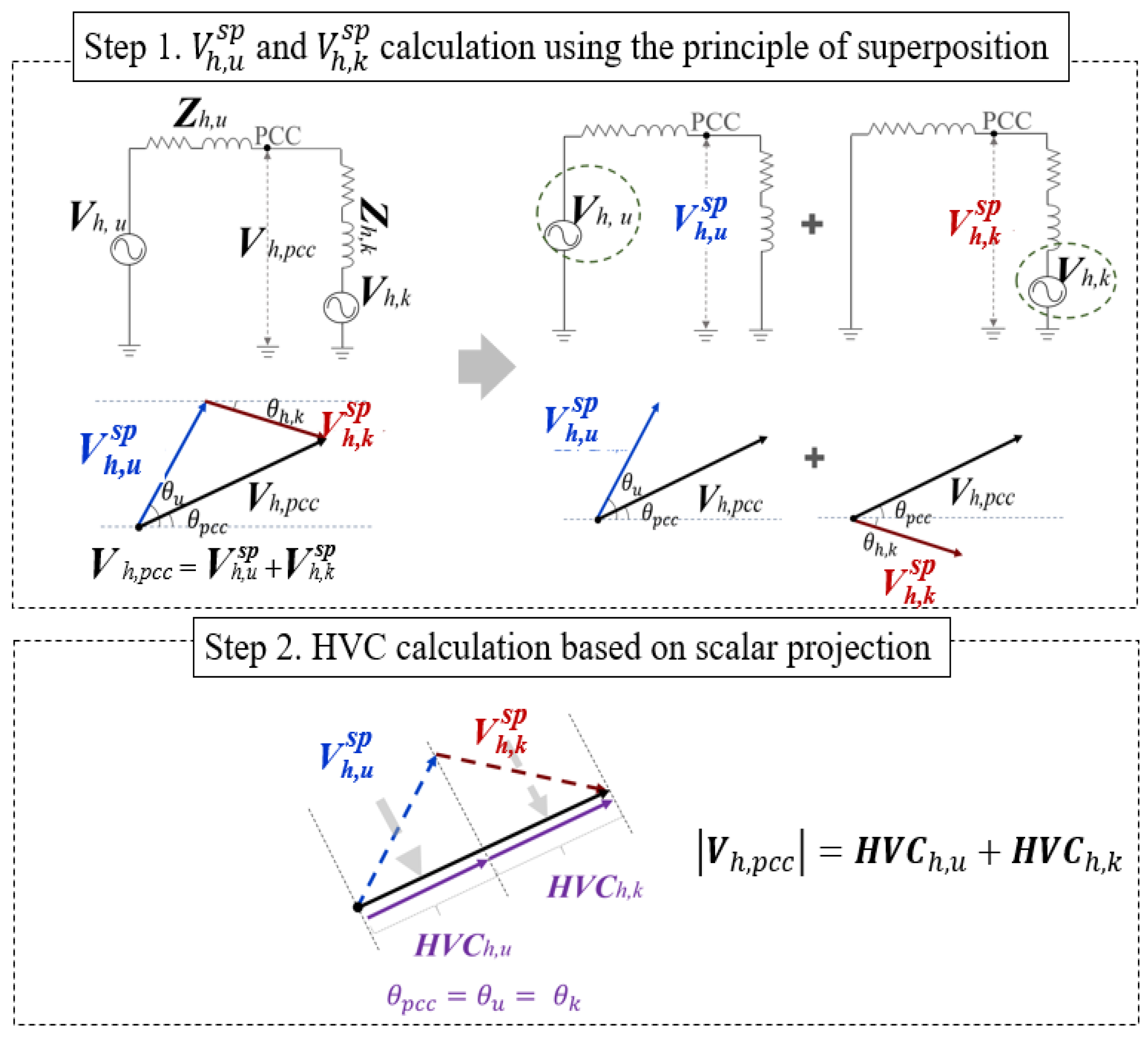
3.1. Harmonic Contribution Assessment Based on the Principle of Superposition

Harmonic contribution assessment requires equivalent voltage models of the utility side and customers connected to PCCs. We can use the proposed method to estimate an individual harmonic customer’s equivalent voltage and impedance. On the other hand, voltage and current measurements on the utility side are basically possible, so the feeder impedance between the utility and PCC can be calculated using Equation (9). If the measurement on the utility side is not possible, the utility’s system impedance can be approximately calculated using a short-circuit analysis program [15].

$$Z_{h,u}=\frac{V_{h,u}-V_{h,pcc} }{I_{h,u}}$$

(9)

where V_h,u and I_h,u are the hth harmonic voltage and current of the utility side.

The PCC voltage of the hth harmonic order in the equivalent model circuit can be represented by the vector sum of the utility voltage of $V_{h,u}^{sp}$ and the customer k voltage of $V_{h,k}^{sp}$, calculated using the principle of superposition, as shown in Figure 6. However, since $V_{h,u}^{sp}$ and $V_{h,k}^{sp}$ are complex vector values, the voltage contribution of the utility and customer k cannot be quantified as a single value. In [16], a method for quantifying the harmonic voltage contribution (HVC) using a scalar dot product was proposed. HVC indicates the contributions of harmonic sources to PCC voltage distortion.

If n-customers are connected to a PCC, $V_{h,u}^{sp}$ and $V_{h,k}^{sp}$ are calculated, as shown in Equations (10)–(13). Then, the PCC voltage of the hth harmonic can be calculated, as in Equation (14).

$$V_{h,k}^{sp}=\frac{Z_{h,k}^{ T} }{ Z_{h,u}+Z_{h,k}^T }\times V_{h,k}$$

(10)

$$V_{h,u}^{sp}=\frac{Z_{h,u}^T }{ Z_{h,u}+Z_{h,u}^T }\times V_{h,u}$$

(11)

$$Z_{h,k}^T={\left[{\left(Z_{h,u}\right)}^{-1}+{{\displaystyle \sum }}_{i=1,i\ne k}^n{\left(Z_{h, i}\right)}^{-1}\right]}^{-1}$$

(12)

$$Z_{h,u}^T={\left[{\displaystyle \sum }_{i=1}^n{\left(Z_{h, i}\right)}^{-1}\right]}^{-1}$$

(13)

$$V_{h,pcc}=V_{h,k}^{sp}+{{\displaystyle \sum }}_{i=1}^n{V}_{h,i}^{sp} (i=1,2,\dots , k,\dots , n)$$

(14)

where $V_{h,u}^{sp}$ and $V_{h,k}^{sp}$ are the hth harmonic voltage contributed by utility and customer k. Moreover, Z_h,u and Z_h,k are the equivalent impedances of the hth harmonic order for the utility and customer k, and V_h,u and V_h,i are the equivalent voltages of the hth harmonic order for the utility u and customer i. $Z_{h,u}^T$ and $Z_{h,k}^T$ represent the impedances as viewed from the utility and customer k at the hth harmonic order, respectively.

Based on the scalar projection, each harmonic source’s hth HVC can be calculated as follows:

$$HV{C}_{h, s}=\frac{ V_{h,s}^{sp}· V_{h,pcc} }{\left|V_{h,pcc}\right|}$$

(15)

where · and | | respectively present the dot product and absolute value. The subscript s represents each harmonic source of the utility u and customer i connected to the PCC.

The harmonic contribution ratio (HCR), which is the ratio of the relative contribution of each harmonic source to the PCC voltage distortion, can also be calculated as follows:

$$HC{R}_{h,s}=\frac{ HV{C}_{h,s} }{\left|V_{h,pcc}\right|}\times 100\%$$

(16)

where HCR_h,s is the HCR of the hth harmonic order for harmonic sources s.

As described above, the HVC and HCR calculations allow us to evaluate the contribution of harmonic sources in individual harmonic orders. However, there is a need for a comprehensive evaluation method that considers all harmonic orders. In [16], the total harmonic contribution (THC) was introduced based on a concept similar to THD. As shown in Equation (17), the THC is defined as the ratio of HVCs for all harmonic orders to the fundamental HVC. THC quantifies the contribution of each harmonic source to PCC voltage distortion for all harmonic orders. The total harmonic contribution ratio (THCR), which is the relative THC of each harmonic source to all sources, is also calculated as shown in Equation (18).

$$TH{C}_s=\frac{\sqrt{ {{\displaystyle \sum }}_{h=2}^{h\_end}{\left(HV{C}_{h, s}\right)}^{2 }}}{\left|\sum HV{C}_{1,s} \right|}\times 100\%$$

(17)

$$THC{R}_s=\frac{TH{C}_s }{ {}_{ }{}^{\forall }THC }\times 100\%$$

(18)

where h_end is the highest harmonic order and THC_S is the total harmonic contribution for the harmonic source s. ^∀THC is the THC sum of all harmonic sources at the PCC and THCRs is the ratio of the relative THC of the harmonic source s to ^∀THC.

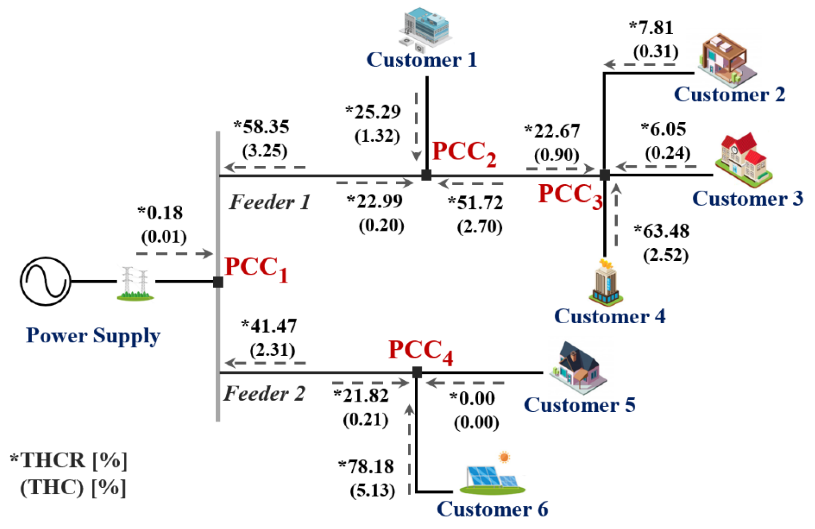
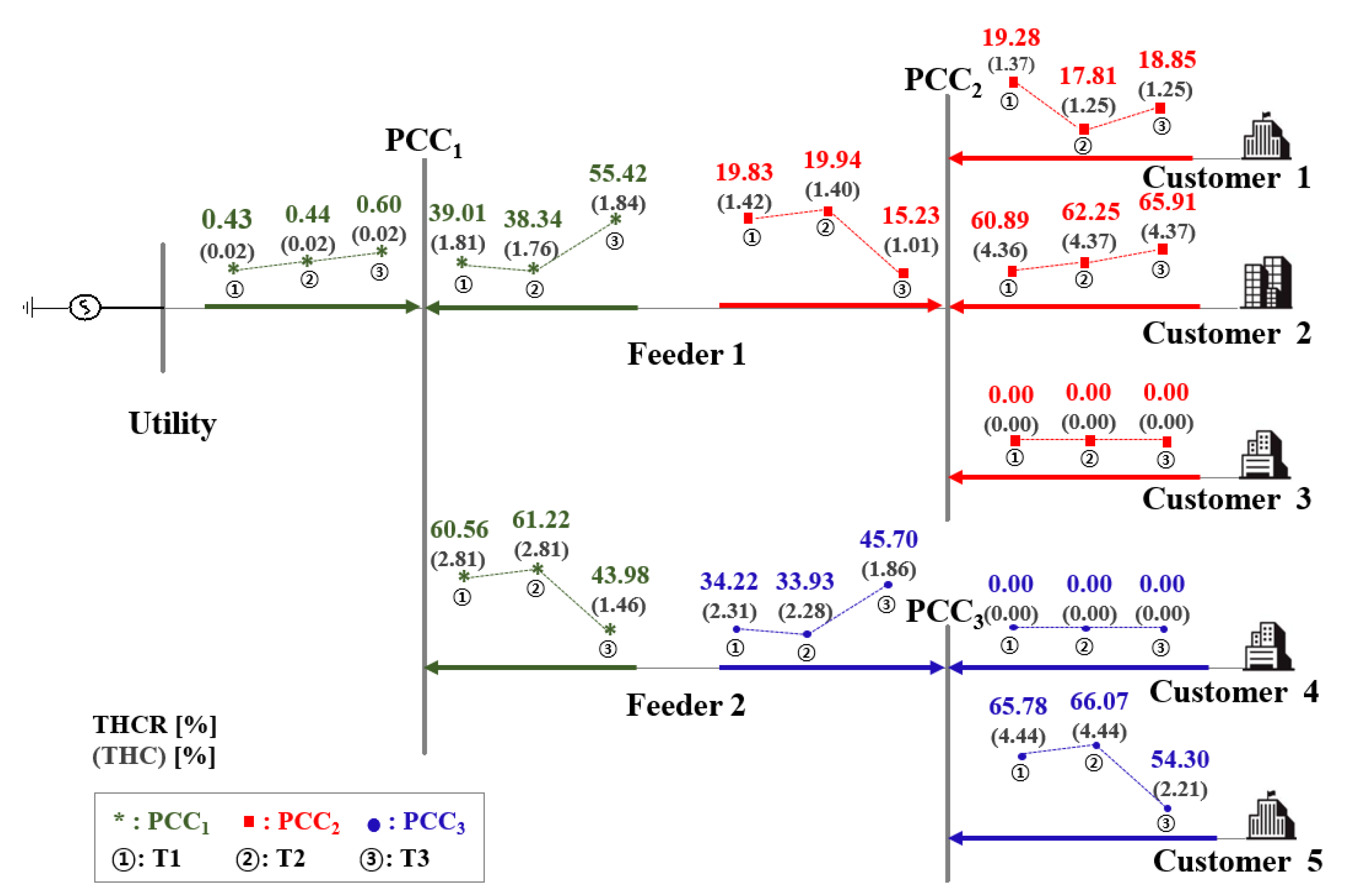
3.2. A Harmonic Contribution Diagram

The harmonic contribution diagram shows the calculated THC and THCR along with a system diagram providing an intuitive understanding of the voltage distortion contributions of harmonic sources. The harmonic contribution diagram can help identify and manage system harmonic levels and sources, causing significant impacts. Using the proposed method, the diagram can be constructed via a sequential evaluation at all system PCCs. Figure 7 shows an example of a harmonic contribution diagram for a distribution system consisting of four PCCs and six customers. For PCC₁, the THCs of feeders 1 and 2 were 3.25% and 2.31%, respectively, and the THCR of feeder 1 was 58.35%, indicating that feeder 1 had a relatively higher contribution to the PCC₁ voltage distortion than utility and feeder 2. For PCC₄, customer 5, with a THC of 0%, did not contribute to the voltage distortion. On the other hand, customer 6, with a THC of 5.13%, showed a larger contribution to the PCC₄ voltage distortion than other harmonic sources.

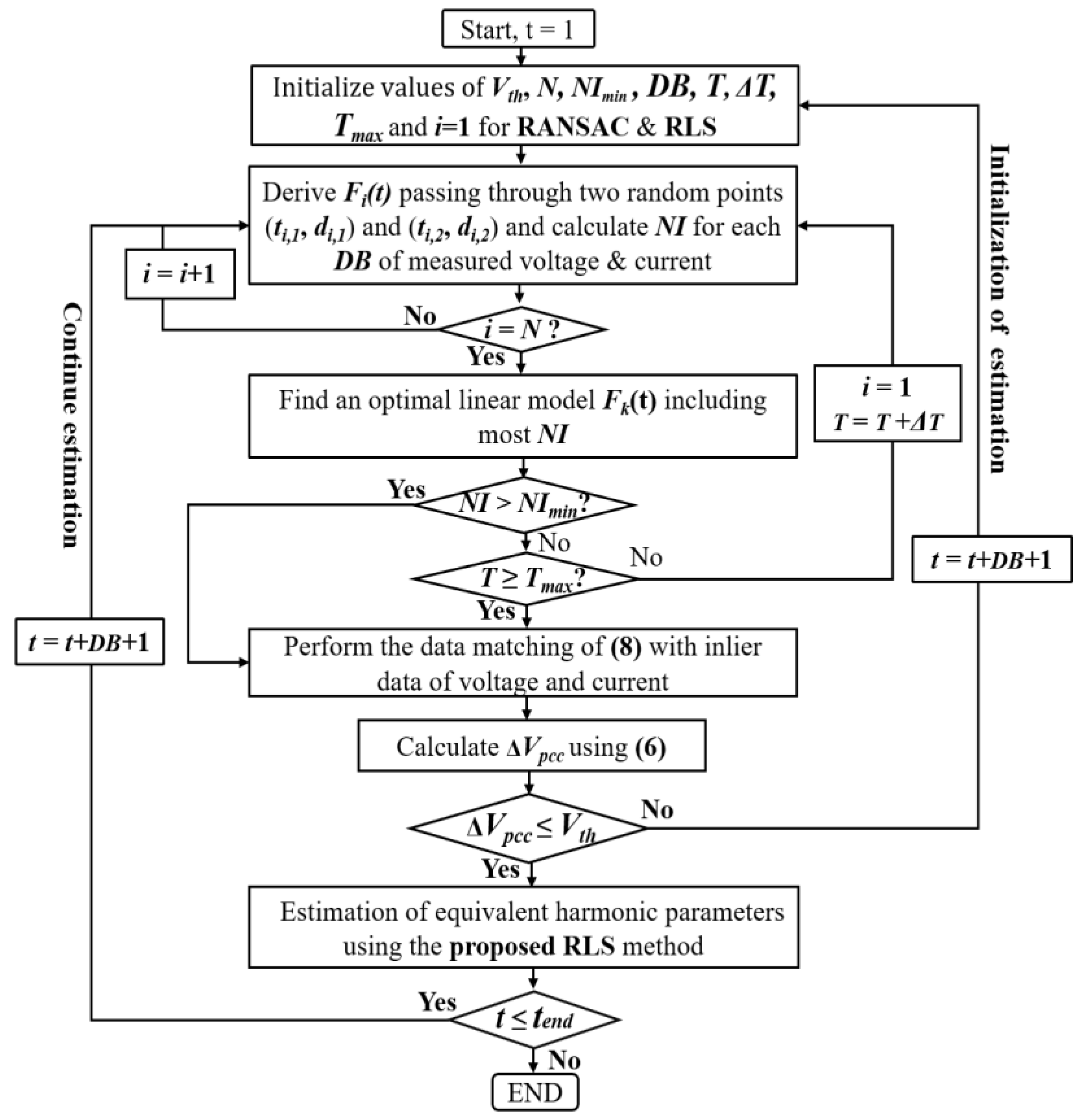
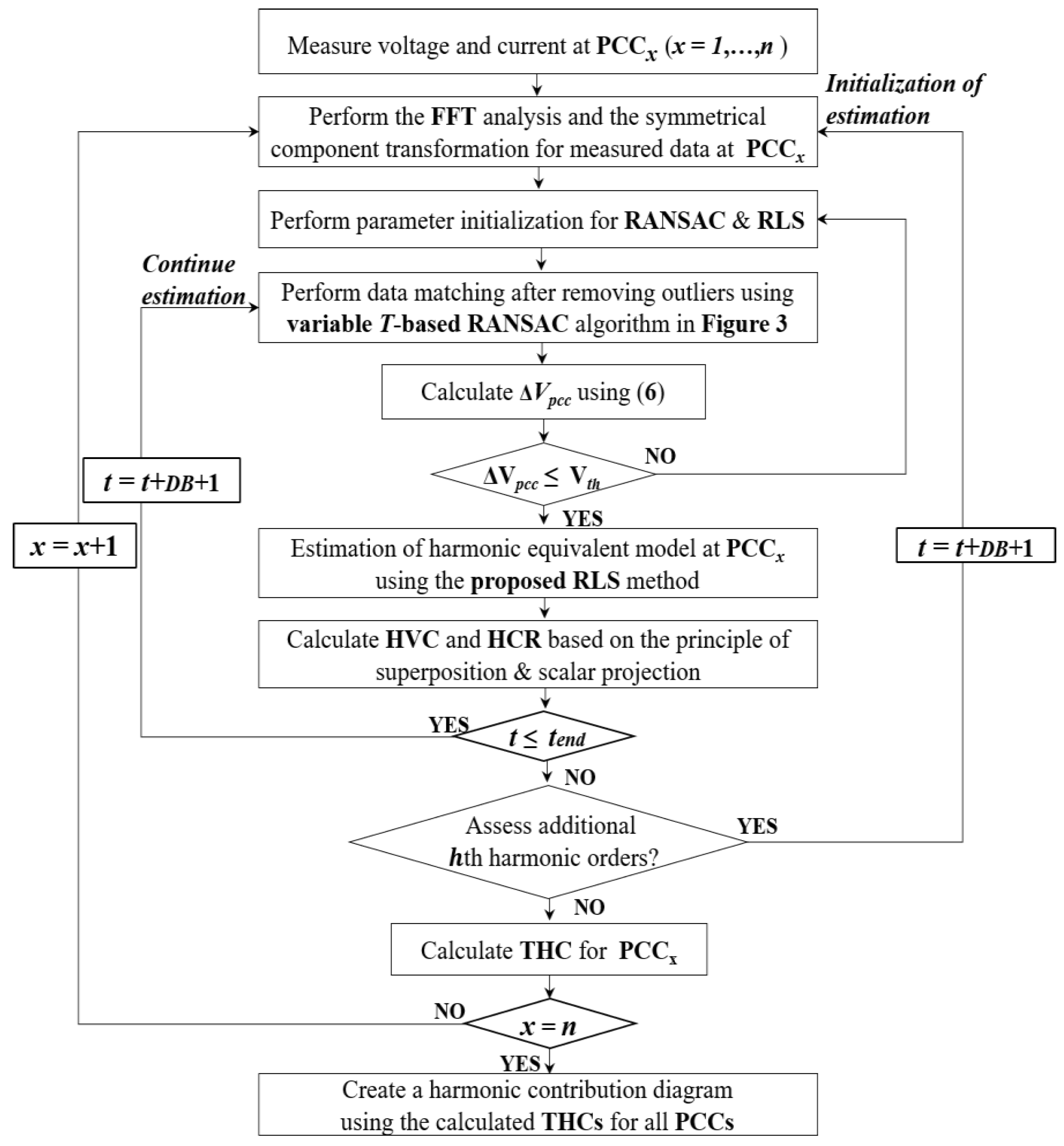
3.3. Entire Procedure of the Proposed Harmonic Contribution Assessment

The entire RANSAC and RLS algorithm-based harmonic contribution assessment procedure is shown in Figure 8. First, we performed an FFT analysis on the voltage and current measured at the PCC and decomposed it into components for each harmonic order. As introduced in [17], we performed symmetric component transformation for each order voltage and current for contribution evaluation under the three-phase unbalanced condition. The proposed RANSAC algorithm, including the variable threshold range scheme, was performed for a certain DB’s voltage and current. After determining an optimal linear model, outliers were removed, and the DB was reconstructed with only the inliers. Then, we completed the RLS estimation input dataset by performing the data matching of Equation (8) on DBs of inlier voltages and currents. Next, by comparing the change rate of PCC voltage of Equation (6) with the threshold value, V_th, the RLS estimation was either initialized or continued. The equivalent voltage models of all harmonic sources were estimated using the RLS algorithm. We then calculated each harmonic source’s HVC and HCR. After performing the HVC evaluation on all harmonic orders, we calculated the THC and THCR using Equations (17) and (18). The above procedure was performed for all PCCs in the system. Finally, we constructed a harmonic contribution diagram using the evaluated THCs and THCRs.

4. Case Study

To verify the proposed method’s performance, we conducted a case study using the PSCAD/EMTDC test system consisting of a utility and five customers, as shown in Figure 9. Customers 1, 2, and 3 are connected to PCC₂, while customers 4 and 5 are connected to PCC₃.

The detailed parameters of the utility and customers are summarized in

Table 1. The initial parameters of utility and the five customers.

Harmonic Order		Utility	Customer 1	Customer 2	Customer 3	Customer 4	Customer 5
Voltage [kV]	1st	12.999 + j2.292	0.000 + j0.000	0.000 + j0.000	0.000 + j0.000	0.000 + j0.000	0.000 + j0.000
	3rd	0.001 + j0.001	1.201 + j0.212	1.398 + j0.247	0.000 + j0.000	0.000 + j0.000	1.753 + j0.309
	5th	0.001 + j0.001	0.709 + j0.125	0.935 + j0.165	0.000 + j0.000	0.000 + j0.000	0.738 + j0.130
	7th	0.001 + j0.001	0.807 + j0.142	0.542 + j0.095	0.000 + j0.000	0.000 + j0.000	0.345 + j0.061
Impedance [Ω]	1st	1.000 + j0.377	4.000 + j3.770	3.000 + j1.131	2.000 + j0.754	3.000 + j0.754	2.000 + j1.131
	3rd	1.000 + j1.131	4.000 + j11.310	3.000 + j3.393	2.000 + j2.262	3.000 + j2.262	2.000 + j3.393
	5th	1.000 + j1.885	4.000 + j18.850	3.000 + j5.655	2.000 + j3.770	3.000 + j3.770	2.000 + j5.655
	7th	1.000 + j2.639	4.000 + j26.389	3.000 + j7.917	2.000 + j5.278	3.000 + j5.278	2.000 + j7.917

. Customers 1, 2, and 5 were modeled as harmonic sources while customers 3 and 4 were modeled as linear loads without harmonic sources.

The total simulation time was 5 s for each case. The voltage and current were measured at 10,000 samples per second and the DB’s size was 40 samples of measured data. Additionally, it was assumed that the equivalent parameters of customers 1 and 5 change, as shown in

Table 2. The equivalent parameter changes on two customers 1 and 5.

Harmonic Order		Customer 1		Customer 5
		0~2 s	2~5 s	0~3.5 s	3.5~5 s
Voltage [kV]	3rd	1.201 + j0.212	0.847 + j0.149	1.753 + j0.309
	5th	0.709 + j0.125	1.104 + j0.195	0.738 + j0.130
	7th	0.807 + j0.142	0.551 + j0.097	0.345 + j0.061
Impedance [Ω]	3rd	4.000 + j11.310		2.000 + j3.393	6.000 + j6.786
	5th	4.000 + j18.850		2.000 + j5.655	6.000 + j11.310
	7th	4.000 + j26.389		2.000 + j7.917	6.000 + j15.834

. Figure 10 shows voltages and currents measured at PCC₁, PCC₂, and PCC₃. Random white noise and outliers were included in the measurement data to achieve realistic conditions.

In this case study, we evaluated the harmonic contributions to voltage distortion at the three PCCs using the proposed method. The outliers were removed using the RANSAC algorithm. Moreover, the equivalent voltage models for all harmonic sources were estimated. Additionally, through HVC and HCR calculations, the harmonic source’s harmonic contribution was evaluated. The harmonic contribution diagram was also derived by calculating THC and THCR considering all harmonic orders.

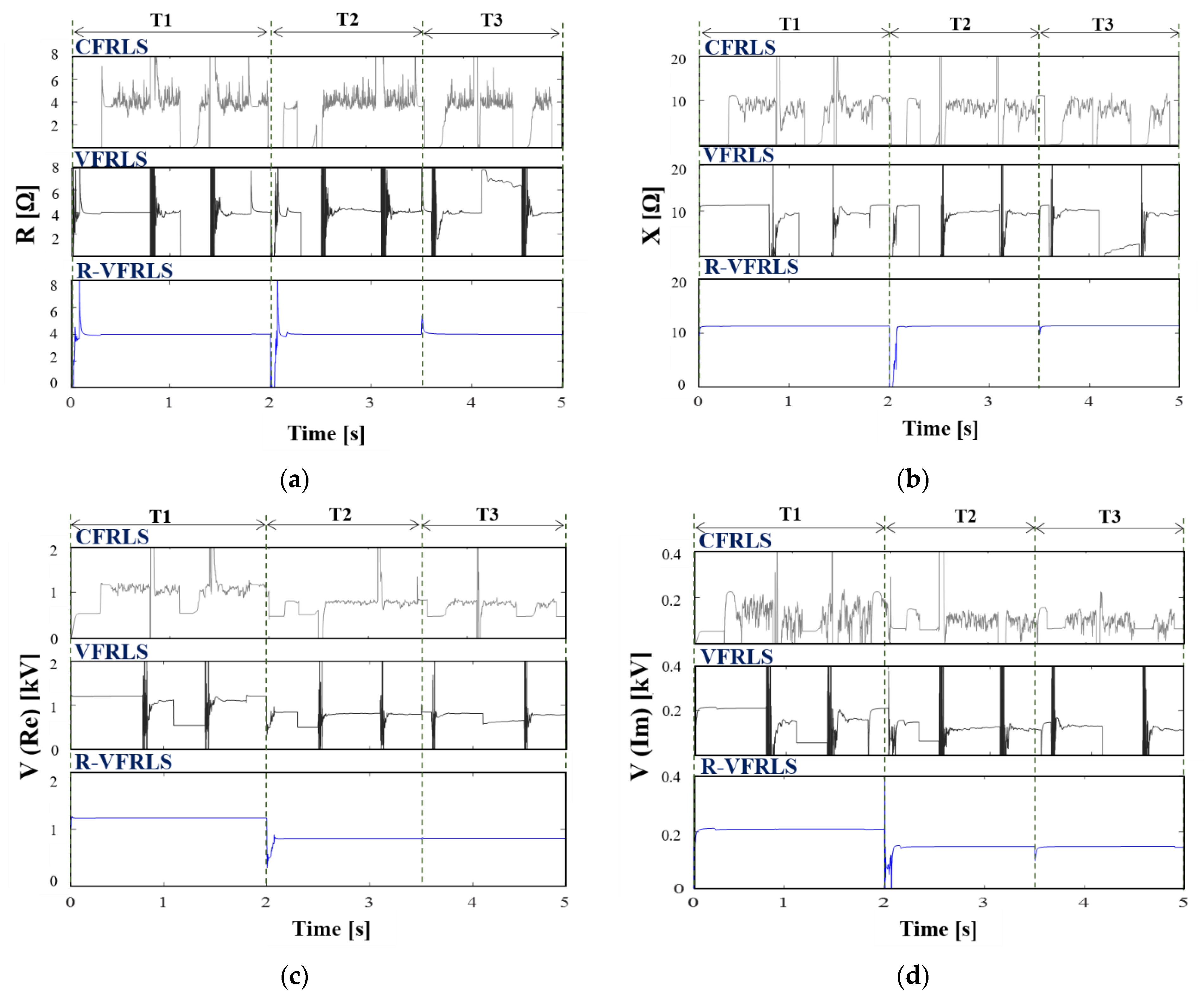
4.1. Equivalent Parameter Estimation Using the Proposed Method

The estimation of an accurate equivalent model for each harmonic order is the most important part of harmonic contribution evaluation. As an example, we analyzed the estimation result of the 3rd harmonic equivalent model of customer 1. To prove the proposed method’s superiority, we performed a comparative analysis with the existing constant forgetting fact RLS (CFRLS) [16] and variable forgetting fact RLS (VFRLS) [17] estimation methods. In the case of customer 1, five outliers were detected and removed for the measured current using the proposed RANSAC algorithm. Considering the outliers in the PCC₂ voltage and the measured currents of customers 1, 2, and 3, a total of 15 data points were excluded through the data matching of Equation (8). We estimated the equivalent model’s voltage source and impedance using the inliers and the proposed RLS algorithm. Figure 11 shows the results of customer 1’s equivalent model estimation using the CFRLS, VFRLS, and the proposed method. According to the parameter detection of Equation (6), for the entire simulation time, parameter estimation was conducted for three time sections: T1, T2, and T3. The CFRLS and VFRLS methods showed very unstable estimation performance for all time sections due to the presence of outliers, while the proposed method showed an overall stable estimation performance even when with the change in parameters.

Table 3. The comparison of 3rd harmonic equivalent parameter estimates for customer 1.

Parameter	Estimation Method	Time Section
		T1			T2			T3
		Estimation	Actual	Error (%)	Estimation	Actual	Error (%)	Estimation	Actual	Error (%)
R [Ω]	CFRLS	9.074	4.000	126.85	7.092	4.000	77.30	14.505	4.000	262.63
	VFRLS	3.426		14.35	3.502		12.45	5.281		32.03
	Proposed	4.002		0.05	3.996		0.10	4.005		0.12
X [Ω]	CFRLS	9.616	11.310	14.98	8.194	11.310	27.55	−3.699	11.310	132.71
	VFRLS	7.066		37.52	7.576		33.01	6.317		44.15
	Proposed	11.282		0.25	11.285		0.22	11.305		0.04
V [kV] (Re)	CFRLS	1.276	1.201	6.24	0.822	0.847	2.95	0.620	0.847	26.80
	VFRLS	0.983		18.15	0.749		11.57	0.734		13.34
	Proposed	1.200		0.08	0.846		0.12	0.847		0.01
V [$\mathrm{kV}$] (Im)	CFRLS	−0.080	0.212	137.74	0.025	0.149	83.22	−0.387	0.149	359.73
	VFRLS	0.110		48.11	0.101		32.21	0.031		79.19
	Proposed	0.211		0.47	0.148		0.67	0.149		0.01

summarizes the average values of the estimation results of the three methods. The CFRLS and VFRLS methods showed large errors between the estimated and actual values, while the proposed method showed very accurate results, with a parameter estimation error rate of less than 1%. The equivalent models for all harmonic sources were estimated using the proposed method.

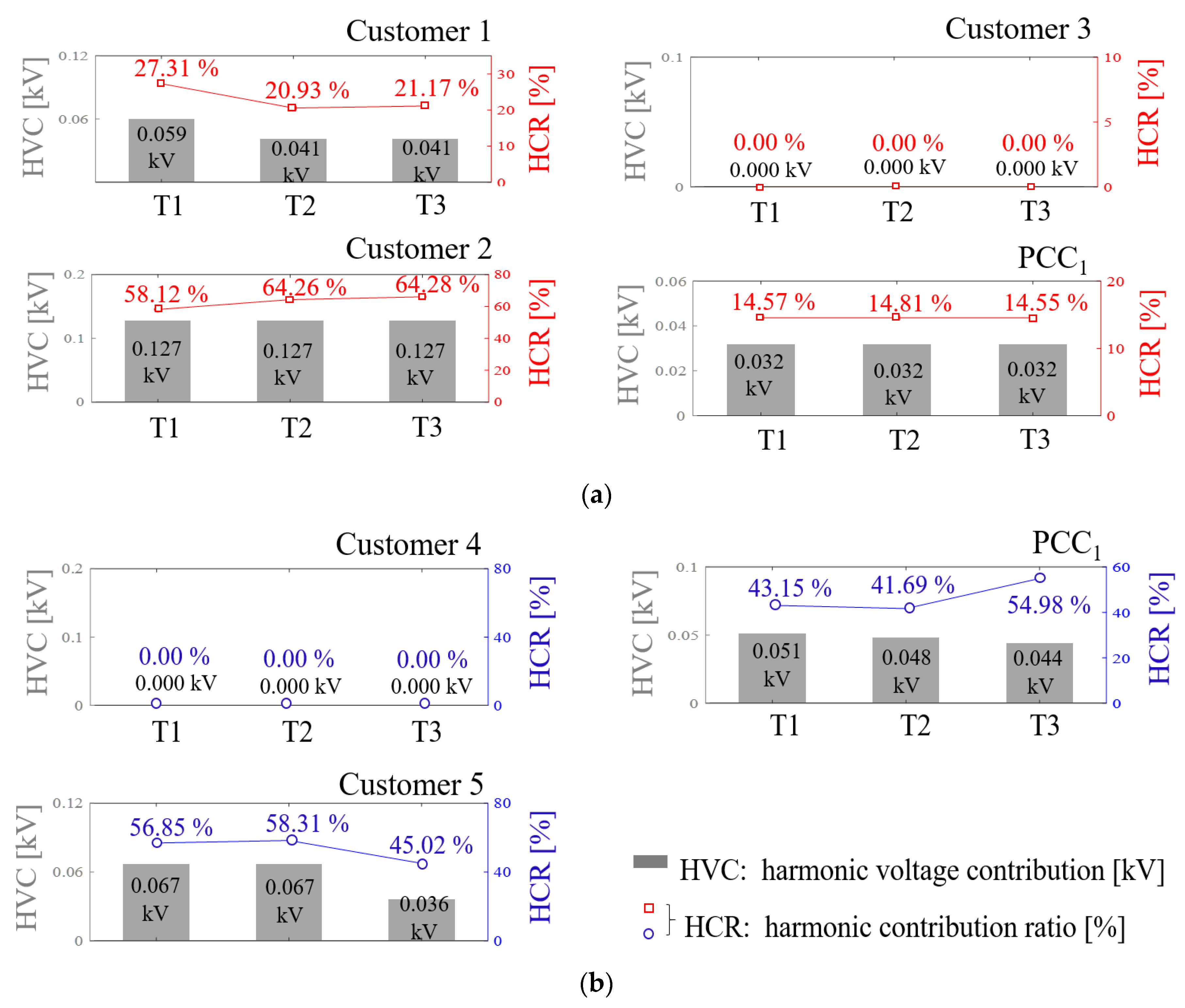
4.2. HVC and HCR Evaluation

As shown in

Table 4. The assessment results of HVC and HCR for the 3rd, 5th and 7th orders.

Harmonic Order	Time Section	Evaluation Index	PCC1			PCC2				PCC3
			Utility	F1	F2	PCC1	C1	C2	C3	PCC1	C4	C5
3rd	T1	HVC	0.00	0.12	0.22	0.12	0.10	0.32	0.00	0.19	0.00	0.39
		HCR	0.33	35.43	64.24	21.51	18.82	59.67	0.00	33.22	0.00	66.78
	T2	HVC	0.00	0.11	0.22	0.11	0.072	0.32	0.00	0.19	0.00	0.39
		HCR	0.38	33.77	65.85	22.31	14.10	63.59	0.00	32.62	0.00	67.38
	T3	HVC	0.00	0.12	0.11	0.08	0.07	0.32	0.00	0.15	0.00	0.19
		HCR	0.51	50.83	48.66	16.68	15.12	68.20	0.00	43.73	0.00	56.27
5th	T1	HVC	0.00	0.08	0.08	0.06	0.05	0.22	0.00	0.09	0.00	0.15
		HCR	0.69	47.48	51.83	17.09	16.43	66.48	0.00	37.88	0.00	62.12
	T2	HVC	0.00	0.09	0.08	0.06	0.09	0.22	0.00	0.10	0.00	0.15
		HCR	0.67	50.12	49.21	16.36	23.32	60.32	0.00	39.11	0.00	60.89
	T3	HVC	0.00	0.09	0.05	0.05	0.09	0.22	0.00	0.09	0.00	52.08
		HCR	0.77	65.57	33.66	13.43	24.12	62.45	0.00	52.11	0.00	47.89
7th	T1	HVC	0.00	0.05	0.04	0.03	0.06	0.13	0.00	0.05	0.00	0.07
		HCR	1.23	57.52	41.25	14.57	27.31	58.12	0.00	43.15	0.00	56.85
	T2	HVC	0.00	0.05	0.04	0.03	0.04	0.13	0.00	0.05	0.00	0.07
		HCR	1.43	54.82	43.75	14.81	20.93	64.26	0.00	41.69	0.00	58.31
	T3	HVC	0.00	0.05	0.02	0.03	0.04	0.13	0.00	0.04	0.00	0.04
		HCR	1.53	69.04	29.43	14.55	21.17	64.28	0.00	54.98	0.00	45.02

Note: F1 and F2 indicate the feeders 1 and 2; C1, C2, C3, C4, and C5 represent the five customers.

, each harmonic source’s HVC and HCR were calculated using the estimated equivalent model and the principle of superposition. The results provide a quantitative understanding of the contributions of harmonic sources to each harmonic order’s PCC voltage distortion. Particularly speaking, the averages of the 7th HVC and HCR estimation results are shown in Figure 12. Figure 12a shows the estimated average HVCs of harmonic sources connected to PCC₂ for each time section. We can observe that customer 2 causes the largest voltage distortion of 0.127 kV in all time sections. On the other hand, customer 3, which is a linear load, does not contribute to the voltage distortion of PCC₂. Figure 12b shows the results of HVCs for PCC₃. For the time sections T1 and T2, customer 5 had the highest HVC of 0.067 kV. For the time section T3, the HVC of customer 5 decreased from 0.067 to 0.036 kV, while PCC₁ showed the highest contribution with an HVC value of 0.044 kV. Through HVC and HCR evaluations, we can quantitatively determine the contributions of harmonic sources to specific harmonic voltage.

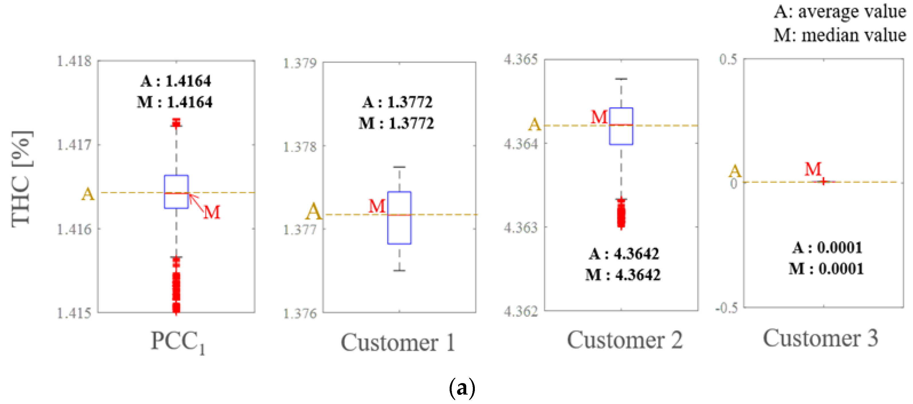
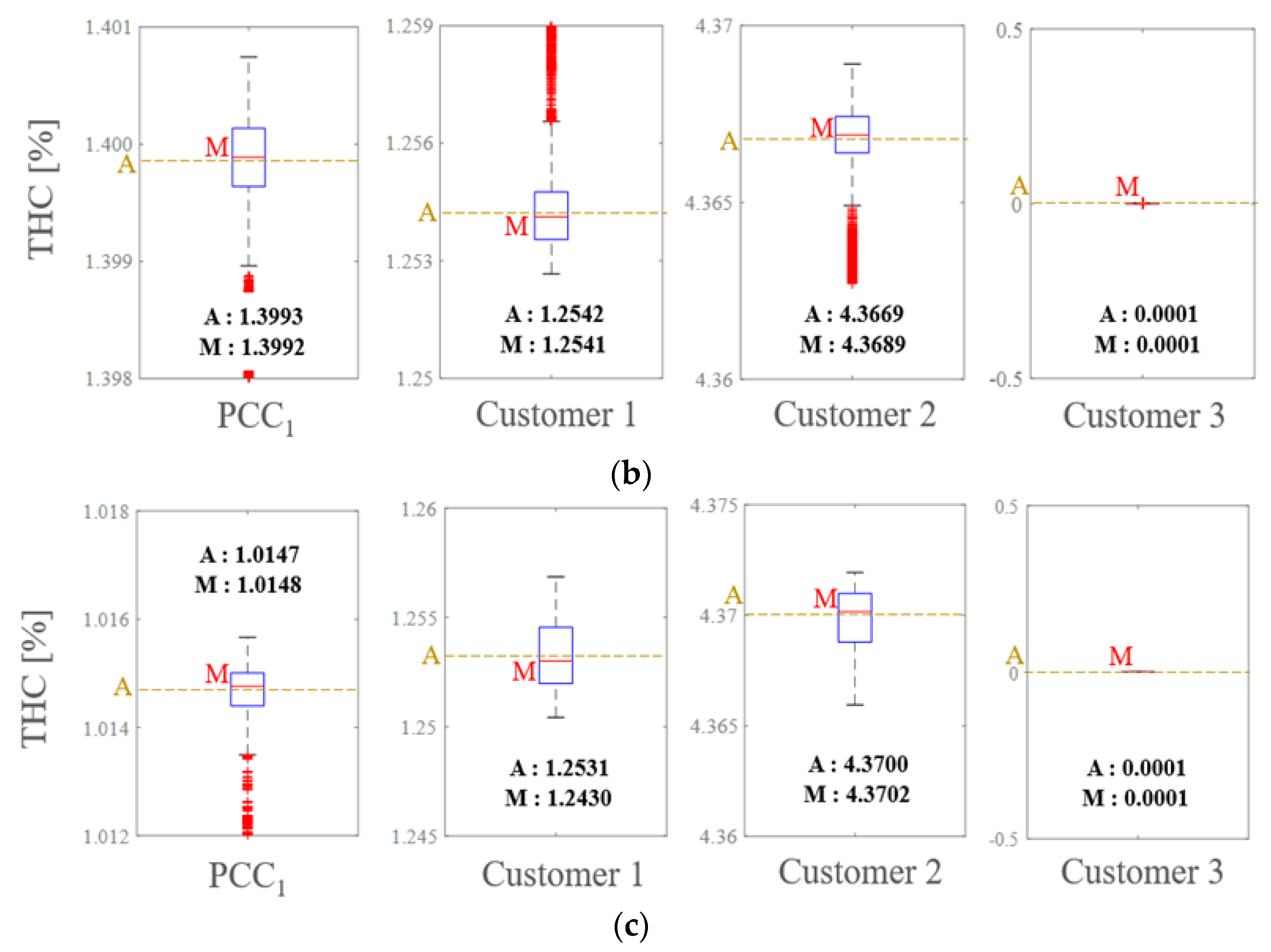
4.3. Creating a Harmonic Contribution Diagram with THC and THCR

To create a harmonic distortion diagram, THC and THCR evaluations were performed for all harmonic sources. The THC and THCR, reflecting the fundamental and all harmonic orders, are calculated using Equations (17) and (18). These indices allow us to grasp the synthesized contributions of all harmonic orders. Figure 13 shows the median and average values of THC corresponding to each time section at PCC₂. We can observe that the deviation between the THC’s median and average values is very small, indicating a very stable estimation performance. The THC of customer 2 was about 4.3% in all time sections, showing the highest contribution to voltage distortion at PCC₂. On the other hand, the THC of customer 3, which is a linear load, was 0%.

For all harmonic sources, we calculated each time section’s THC and THCR. The harmonic contribution diagram was completed, as shown in Figure 14. From the diagram, we can intuitively determine that for the case of PCC₁, the THC and THCR on the feeder 2 side are relatively high for time sections T1 and T2, indicating the highest contribution to voltage distortions. However, for the time section T3, the THC and THCR of the feeder 2 side decreased, and the harmonic contribution of the feeder 1 side was the highest. Based on these harmonic evaluations, we can identify harmonic sources that cause severe system voltage distortions and effectively manage these harmonics.

5. Conclusions

This paper presented an advanced method of harmonic contribution assessment based on the RANSAC and RLS methods. In the parameter estimation of harmonic equivalent models, there is a problem that the estimation performance is significantly deteriorated when outliers exist in measured data. The proposed method effectively detects and removes outliers using the RANSAC algorithm and performs equivalent model estimation and harmonic contribution evaluation using only inliers, which shows superior performance than existing methods. In addition, a method for creating a harmonic contribution diagram that can effectively identify harmonic sources in a distribution system was proposed. By displaying the THC and THCR evaluation results at each common coupling point along with a system diagram, the contributions of harmonic sources to PCC voltage distortion can be intuitively understood. Along with the advancement of monitoring and measuring technology, the proposed method can be effectively used for system harmonic management and establishment of mitigation measures.

References

1. Manito, A.; Bezerra, U.; Tostes, M.; Matos, E.; Carvalho, C.; Soares, T. Evaluating Harmonic Distortions on Grid Voltages Due to Multiple Nonlinear Loads Using Artificial Neural Networks. Energies 2018, 11, 3303. [Google Scholar] [CrossRef]
2. Singh, R.S.; Ćuk, V.; Cobben, S. Measurement-Based Distribution Grid Harmonic Impedance Models and Their Uncertainties. Energies 2020, 13, 4259. [Google Scholar] [CrossRef]
3. Rüstemli, S.; Okuducu, E.; Almalı, M.N.; Efe, S.B. Reducing the effects of harmonics on the electrical power systems with passive filters. Bitlis Eren Univ. J. Sci. Technol. 2015, 5, 1–10. [Google Scholar] [CrossRef]
4. Michalec, Ł.; Jasiński, M.; Sikorski, T.; Leonowicz, Z.; Jasiński, Ł.; Suresh, V. Impact of Harmonic Currents of Nonlinear Loads on Power Quality of a Low Voltage Network–Review and Case Study. Energies 2021, 14, 3665. [Google Scholar] [CrossRef]
5. Chen, H.; Guo, T.; Zhang, L. Comparative Study of Power Loss and Thermal Performance in Five-Phase FSCWPM Machine With/Without Third Harmonic Current Injection. J. Electr. Eng. Technol. 2021, 16, 2099–2108. [Google Scholar] [CrossRef]
6. Park, J.I.; Park, C.H. A study on the application of the recursive least square method for estimating harmonic load model. Trans. Korean Inst. Electr. Eng. 2019, 68, 827–833. [Google Scholar] [CrossRef]
7. Jia, X.; Hua, H.; Cao, D.; Zhao, C. Determining Harmonic Contributions Based on Complex Least Squares Method; Chinese Society of Electrical Engineering: Beijing, China, 2013; Volume 33. [Google Scholar]
8. Sahoo, H.K.; Sharma, P.; Rath, N.P. Robust harmonic estimation using forgetting factor RLS. In Proceedings of the 2011 Annual IEEE India Conference, Hyderabad, India, 16–18 December 2011; pp. 1–5. [Google Scholar]
9. Hua, H.; Liu, Z.; Jia, X. Partially linear model for harmonic contribution determination. IEEJ Trans. Electr. Electron. Eng. 2016, 11, 285–291. [Google Scholar] [CrossRef]
10. Giuseppe, F.; Arturo, L.; Mario, R. Constrained least squares methods for parameter tracking of power system steady-state equivalent circuits. IEEE Trans. Power Del. 2000, 15, 1073–1080. [Google Scholar]
11. Park, J.I.; Park, C.H. A Study on the Parameter Estimation of Harmonic Equivalent Model Using the RANSAC and Recursive Least Square Algorithms. Trans. Korean Inst. Electr. Eng. 2021, 70, 269–275. [Google Scholar] [CrossRef]
12. Sha, H.; Mei, F.; Zhang, C.; Pan, Y.; Zheng, J.; Li, T. Multi-Harmonic Sources Harmonic Contribution Determination Based on Data Filtering and Cluster Analysis. IEEE Access 2019, 7, 85276–85285. [Google Scholar] [CrossRef]
13. Liu, Z.; Xu, Y.; Jiang, H.; Tao, S. Study on Harmonic Impedance Estimation and Harmonic Contribution Evaluation Index. IEEE Access 2020, 8, 59114–59125. [Google Scholar] [CrossRef]
14. Sun, Y.; Li, S.; Xu, Q.; Xie, X.; Jin, Z.; Shi, F.; Zhang, H. Harmonic Contribution Evaluation Based on the Distribution-Level PMUs. IEEE Trans. Power Deliv. 2021, 36, 909–919. [Google Scholar] [CrossRef]
15. De Andrade, G.V., Jr.; Naidu, S.R.; Neri, M.G.G.; da Costa, E.G. Estimation of the utility’s and consumer’s contribution to harmonic distortion. IEEE Trans. Instrum. Meas. 2009, 58, 3817–3823. [Google Scholar] [CrossRef]
16. Han, J.H.; Lee, K.; Song, C.S.; Jang, G.; Byeon, G.; Park, C.H. A new assessment for the total harmonic contributions at the point of common coupling. J. Electr. Eng. Technol. 2014, 9, 6–14. [Google Scholar] [CrossRef]
17. Park, J.I.; Lee, H.; Yoon, M.; Park, C.H. A Novel Method for Assessing the Contribution of Harmonic Sources to Voltage Distortion in Power Systems. IEEE Access 2020, 8, 76568–76579. [Google Scholar] [CrossRef]
18. Zou, M.; Djokic, S.Z. A Review of Approaches for the Detection and Treatment of Outliers in Processing Wind Turbine and Wind Farm Measurements. Energies 2020, 13, 4228. [Google Scholar] [CrossRef]
19. Chen, H.; Li, F.; Wang, Y. Wind power forecasting based on outlier smooth transition autoregressive GARCH model. J. Mod. Power Syst. Clean Energy 2018, 6, 532–539. [Google Scholar] [CrossRef]
20. Zou, M.; Fang, D.; Djokic, S.; Hawkins, S. Assessment of wind energy resources and identification of outliers in on-shore and off-shore wind farm measurements. In Proceedings of the 3rd International Conference on Offshore Renewable Energy (CORE), Glasgow, UK, 29–30 August 2018. [Google Scholar]
21. Gupta, M.; Gao, J.; Aggarwal, C.C.; Han, J. Outlier Detection for Temporal Data: A Survey. IEEE Trans. Knowl. Data Eng. 2014, 26, 2250–2267. [Google Scholar] [CrossRef]
22. Choi, S.; Kim, T.; Yu, W. Performance evaluation of RANSAC family. In Proceedings of the British Machine Vision Conference (BMVC 2009), London, UK, 7–10 September 2009. [Google Scholar]
23. Won, N.K.; Jung, W.W.; Shin, C.H.; Hwang, P.I.; Jang, G. Voltage Control of Distribution Networks to Increase their Hosting Capacity in South Korea. J. Electr. Eng. Technol. 2021, 16, 1305–1312. [Google Scholar]
24. Urdea, M.I.; Anca Elena, N.; Paul, C. The influence of the network impedance on the non-sinusoidal (harmonic) network current and flicker measurements. IEEE Trans. Instrum. Meas. 2011, 60, 2202–2210. [Google Scholar]
25. Wenpeng, L.; Joshua, P.; Mirjana, M.; Joyce, L.; Brian, H. Smart meter data analytics for distribution network connectivity verification. IEEE Trans. Smart Grid 2015, 6, 1964–1971. [Google Scholar]
26. Li, S.; Kaile, Z.; Xiaoling, Z.; Shanlin, Y. Outlier Data Treatment Methods Toward Smart Grid Applications. IEEE Access 2018, 6, 39849–39859. [Google Scholar]
27. Peng, Y.; Yang, Y.; Xu, Y.; Xue, Y.; Song, R.; Kang, J.; Zhao, H. Electricity Theft Detection in AMI Based on Clustering and Local Outlier Factor. IEEE Access 2021, 9, 107250–107259. [Google Scholar] [CrossRef]
28. Jaime, Y.; Bo, T. Detection of Electricity Theft in Customer Consumption Using Outlier Detection Algorithms. In Proceedings of the 2018 1st International Conference on Data Intelligence and Security (ICDIS), South Padre Island, TX, USA, 8–10 April 2018; pp. 135–140. [Google Scholar]
29. Fischler, M.A.; Bolles, R.C. Random Sample Consensus: A Paradigm for Model Fitting with Applications to Image Analysis and Automated Cartography. Commun. ACM 1981, 24, 381–395. [Google Scholar] [CrossRef]
30. Wu, W.; Liu, W. An Optimized Method Based on RANSAC for Fundamental Matrix Estimation. In Proceedings of the 2018 IEEE 3rd International Conference on Signal and Image Processing (ICSIP), Shenzhen, China, 13–15 July 2018; pp. 372–376. [Google Scholar]
Figure 1. An example of a distribution network. (a) Data measurement. (b) The network’s equivalent harmonic voltage model.
Energies 15 06448 g001
Figure 2. The RANSAC algorithm for detecting and removing outliers.
Energies 15 06448 g002
Figure 3. The estimation procedure of equivalent model parameters.
Energies 15 06448 g003
Figure 4. The inliers determination based on the variable T range.
Energies 15 06448 g004
Figure 5. Data matching for PCC voltage and currents.
Energies 15 06448 g005
Figure 6. The harmonic contribution to the PCC voltage based on the principle of superposition and scalar projection.
Energies 15 06448 g006
Figure 7. Example of a harmonic contribution diagram.
Energies 15 06448 g007
Figure 8. The entire procedure of harmonic contribution assessment based on the proposed method.
Energies 15 06448 g008
Figure 9. The PSCAD/EMTDC test system for harmonic contribution assessment.
Energies 15 06448 g009
Figure 10. The measured voltage and currents at each PCC. (a) The PCC1 voltage and the currents of feeders 1 and 2. (b) The PCC2 voltage and the currents of customers 1, 2, and 3. (c) The PCC3 voltage and the currents of customers 3 and 4.
Energies 15 06448 g010aEnergies 15 06448 g010b
Figure 11. The results of the 3rd harmonic parameter estimation for customer 1 by the CFRLS, VFRLS, and proposed method. (a) Resistance. (b) Reactance. (c) The real value of voltage. (d) The imaginary value of voltage.
Energies 15 06448 g011
Figure 12. The assessment results of the 7th HVC and HCR. (a) PCC2. (b) PCC3.
Energies 15 06448 g012
Figure 13. The results of the THC assessment for PCC2. (a) The average and median values of THC for the time section T1. (b) The average and median values of THC for time section T2. (c) The average and median values of THC for the time section T3.
Energies 15 06448 g013aEnergies 15 06448 g013b
Figure 14. The harmonic contribution diagram displaying the estimated THC and THCR.
Energies 15 06448 g014