Article

An Output Feedback Discrete-Time Controller for the DC-DC Buck Converter

by
Martin A. Alarcón-Carbajal
1,†,
José E. Carvajal-Rubio
2,3,†,
Juan D. Sánchez-Torres
4,†,
David E. Castro-Palazuelos
1,† and
Guillermo J. Rubio-Astorga
1,*,†
1
División de Estudios de Posgrado e Investigación, Tecnológico Nacional de México/IT de Culiacán, Culiacán 80220, Mexico
2
Departamento de Control Automatico, CINVESTAV, Zapopan 45019, Mexico
3
LAMIH, INSA, Université Polytechnique Hauts-de-France, 59313 Valenciennes, France
4
Department of Mathematics and Physics, ITESO, San Pedro Tlaquepaque 45604, Mexico
*
Author to whom correspondence should be addressed.
These authors contributed equally to this work.
Energies 2022, 15(14), 5288; https://doi.org/10.3390/en15145288
Submission received: 15 June 2022 / Revised: 2 July 2022 / Accepted: 19 July 2022 / Published: 21 July 2022
(This article belongs to the Section F3: Power Electronics)

Abstract

:
This paper presents a discrete-time output feedback controller to regulate the output voltage of a DC-DC buck converter. The proposal’s main feature is the application of a discrete-time equivalent of the robust exact filtering differentiator. First, the document exposes a theoretical analysis of the closed-loop system, where it is considered the problem of implementing a real-time differentiator with a good relationship between exactness and noise filtration performance. Hence, secondly, the controller in a laboratory setup is presented. The first experimental results suggest that the proposed controller exhibits good robustness against noise and maintains the asymptotic accuracy, even with saturated control inputs, as in the case of the DC-DC buck converter. Consequently, aiming to verify the features of the proposed method, the controller is validated through multiple experiments, showing satisfactory voltage tracking accuracy, good suppression of instantaneous load and supply voltage disturbances, and robustness against bounded measurement noise.

1. Introduction

Nowadays, DC-DC switching converters are present in most branches of engineering, and industry [1,2]. It is common to find applications of DC-DC switching converters in aerospace systems [3,4], automotive electronics [5,6,7], uninterruptible power supplies (UPS) [8,9] and especially in renewable energy systems, such as fuel cells [10,11], photovoltaic systems [12,13,14,15] and wind power [16,17] just to mention a few. The main characteristic of a DC-DC switching converter is the ability to ensure a constant output voltage for the entire operating range, even in the presence of variations in the supply voltage and non-constant power demand. Additionally, it is well known that these devices exhibit nonlinear phenomena, and most of them operate in adverse conditions due to commutation noise and other electromagnetic effects [18]. Therefore, the design of closed-loop feedback control strategies that ensure the correct operation of DC-DC switching converters is crucial.
The most common non-linearity in almost every physical system is the saturation of the control input. In the case of the DC-DC switching converters, this restriction is in the duty cycle that modulates the discontinuous activation signal of the switches [19,20].
Over the years, multiple authors have proposed discrete-time and continuous-time control strategies to deal with the nonlinear dynamics and disturbances that the operation of DC-DC switching converters exhibits. In [21], a comparison between a generalized proportional integral (GPI) controller and a proportional integral derivative (PID) controller implemented on a field-programmable gate array (FPGA) is presented. In [22], the authors present a fractional-order PID-type controller designed explicitly for DC-DC boost converter and implemented in discrete-time using a floating-point digital signal processor (DSP). In [23], a discrete global-sliding mode (SM) control of DC-DC switching converters is presented and experimentally validated using a DC-DC buck converter. In [24], a digital control based on fuzzy logic for the DC-DC buck converter with photovoltaic applications is presented and validated through experimentation with low-cost digital platforms. In [25], the authors propose finite-time output feedback control with a current sensorless mode for the DC-DC buck converter, which is validated through experimentation. The discrete-time controllers proposed in [21,22,23,24,25], show satisfactory results. However, a detailed analysis of the control signal restrictions caused by duty cycle saturation is not performed. Due to its complexity, it is common to neglect this phenomenon. However, it should be considered to ensure the stability of the closed-loop control system.
On the other hand, few papers analyze the saturation of the control input in DC-DC switching converters and its effect on the system’s stability. For example, in [26] a Lyapunov-based proportional-integrative (PI) controller with Δ Σ modulator for the DC-DC buck converter with saturated input is presented and experimentally validated. In [27], the authors propose a regional pole placement controller that considers the saturation of the duty cycle for the DC-DC buck converter. In [28], a regulator based on the closed-loop frequency response of the DC-DC buck converter is presented. The controller is designed by considering the effects of system saturation and validated through numerical simulations. In [29], the author presents a class of proportional-integral with anti-windup (PIAW) controllers for the DC-DC buck converter. The controller considers the limitations of the control input together with detailed stability analysis and is validated through experimentation. In [30], a nonlinear PID regulator to avoid the windup effect with a saturation function for the control signal is presented and validated by simulation. The control strategies mentioned in [26,27,28,29,30] show a satisfactory regulation of the switched DC-DC converters dynamics and analyze the effects of the saturation on the stability of the system.
Nevertheless, most are based on continuous-time controllers and do not explore the effects on stability when the algorithm is implemented on discrete-time platforms. Likewise, the adverse effects that measurement noise has on the control loop are not directly addressed, especially in controllers with derivative actions. As previously mentioned, noise in DC-DC switching converters is a common situation and should be treated with special attention.
One option to estimate those states for systems with noisy output and unavailable states is a differentiator. Specifically, the homogeneous differentiator shows remarkable properties, which have been implemented in different areas [31,32]. They are finite-time convergence, accuracy, and robustness to noise [33,34]. These properties are obtained if the n-th derivative of the free-noise signal has a known Lipschitz constant [33] and bounded noise. Despite the asymptotic accuracy of the well-known robust exact differentiator [33], this accuracy was improved by the robust exact filtering differentiator [34]. On the other hand, the robust exact filtering differentiator used to be implemented in digital systems, but it is a continuous-time observer. For this reason, some discrete-time realization [34,35,36], which preserves the continuous-time properties of the differentiator. One strategy to obtain a discrete-time realization is the implicit discretization [37]. Implicit realizations supersede the explicit discrete-time differentiators based on homogeneous differentiators [35,38,39].
This paper proposes and experimentally validates an output feedback discrete-time controller based on the implicit discretization of the robust exact filtering differentiator. The main advantage of this controller lies in the estimation accuracy of the system states in the presence of measurement noise and its finite-time convergence. The contributions of this paper are as follows:
  • The presentation of a discrete-time output feedback controller based on the robust exact filtering differentiator for the DC-DC buck converter with saturated input.
  • The introduction of a rigorous stability analysis of the discrete-time controller considering the asymmetric saturation of the system.
  • An extensive experimental analysis that includes various operating conditions and disturbance scenarios to validate the performance of the controller.
The difference of this paper with respect to previous research is that the proposed discrete-time controller has the properties of finite-time convergence, accuracy, and robustness to noise of the homogeneous differentiator. It demonstrates that this controller allows the states convergence even with instantaneous reference voltage changes, load disturbances and supply voltage variations. Likewise, for the first time, the closed-loop stability of the the implicit realization of the robust exact filtering differentiator and DC-DC buck converter is analyzed considering the saturation of the duty cycle. It is important to remark that the discrete-time implementation of homogeneous differentiators is a relatively new research topic. However, there are not enough experimental results in the literature about its use in a closed-loop controller.
This paper is organized as follows. In Section 2, the robust exact filtering differentiator and its implicit discretization for discrete-time implementations are presented. In Section 3, the topology of the DC-DC buck converter is analyzed, and its mathematical model based on the classical averaged technique is presented. In Section 4, the proposed control strategy based on the robust exact filtering differentiator is presented, as well as its closed-loop stability analysis considering the saturation of the control signal of the DC-DC buck converter. In Section 5, the experimental results of the controller implemented employing a digital platform in a prototype of the DC-DC buck converter are shown. Finally, the conclusions are presented in Section 6.

2. Robust Exact Filtering Differentiator

Let us consider a signal f 0 t , f 0 : R R , which is assumed to be at least n t h differentiable, and f 0 n t has a known Lipschitz constant L > 0 . Hence, one obtains f 0 n + 1 t L , L almost everywhere. Therefore, the differentiation problem is equivalent to estimate the states of the following continuous-time system:
x ˙ = A x + e n + 1 f 0 ( n + 1 ) ( t ) , f 0 ( t ) = e 1 T x ,
where the state variables are defined as x = x 0 x 1 x 2 x n T R n + 1 with x i = f 0 ( i ) ( t ) , e 1 = 1 0 0 0 T , e n + 1 = 0 0 0 1 T and A is given by
A = 0 1 0 0 0 0 1 0 0 0 0 1 0 0 0 0 .
For system (1), its noisy output, x ¯ 0 ( t ) , is defined as x ¯ 0 ( t ) = x 0 ( t ) + Δ ( t ) . Concerning the noise Δ ( t ) , it satisfies the following assumption:
Assumption 1.
The measurement noise can be represented by n f + 1 components, i.e., Δ ( t ) = Δ 0 ( t ) + Δ 1 ( t ) + + Δ n f ( t ) , where each possibly unbounded component Δ j ( t ) ( j = 0 , 1 , , n f ) is a signal of global filtering order j and the jth-order integral magnitude δ j 0 .
Here, it is recalled the definition of a signal of global filtering order j introduced in [34].
Definition 1
([34]). A function Δ j ( t ) , Δ j : 0 , R , is a signal of global filtering order j 0 , if Δ j is a locally integrable Lebesgue-measurable function, and there exists a globally bounded solution β j ( t ) of the equation β j ( j ) ( t ) = Δ j ( t ) . Any number greater than sup | β j ( t ) | is called a j t h -order global integral magnitude of δ j .
Assumption 1 was introduced in [40]. This assumption is more general than the consideration that Δ ( t ) is a Lebesgue-measurable bounded noise. Indeed, this classical assumption corresponds to the case n f = 0 . Considering system (1) and Assumption 1, the states of the systems can be estimated in real time using the robust exact filtering differentiator, which was originally presented in [34]:
w ˙ j f = ϕ j f 1 , m w 1 + w j f + 1 , w ˙ n f = ϕ n f 1 , m w 1 + z 0 x ¯ 0 , z ˙ j d = ϕ n f + j d , m w 1 + z j d + 1 , z ˙ n = ϕ m , m w 1 . j f = 1 , 2 , , n f 1 . j d = 0 , 1 , 2 , , n 1 ,
where m = n + n f , ϕ j , m · = λ m j L j + 1 m + 1 · m j m + 1 , w j are the states of the filtering part, z j are the robust estimations of the state x j . The parameters λ i are appropriate positive constants. Note that the solution of system (2) is understood in the Filippov sense [41]. Then after a finite-time, the filtering differentiator (2) satisfies the accuracy:
| σ j t | μ j L ρ n + 1 j , μ j > 0 , j = 0 , 1 , 2 , , n . ρ = max δ 0 L 1 n + 1 , δ 1 L 1 n + 2 , , δ n f L 1 m + 1 ,
where σ j ( t ) = z j ( t ) x j ( t ) . The above was demonstrated in [34]. Furthermore, if there exists a positive integer n a > n such that f 0 ( n a + 1 ) ( t ) L , then the accuracy of (3) can be improved using a differentiator of order n a (instead of n). On the other hand, if n f = 0 , then the accuracy of (3) becomes the asymptotic accuracy.

Implicit Discretization of the Robust Exact Filtering Differentiator

Some discrete-time realizations have been presented for the filtering differentiator (2) [34,35,39]. In this paper, the implicit discrete-time differentiator presented in [42] are implemented. Moreover, the states, the noise and signals at time t k are defined as Δ k = Δ ( t k ) , w j , k = w j ( t k ) , z j , k = z j ( t k ) , x j , k = x j ( t k ) , σ j , k = σ j ( t k ) . For discrete-time measurements, the following condition about the noise is considered:
Assumption 2.
The sampled measurement noise consists of n f + 1 components, Δ k = Δ 0 , k + Δ 1 , k + + Δ n f , k , where each possibly unbounded Δ j , k ( j = 0 , 1 , , n f ) is a discretely sampled signal of global filtering order j and jth-order integral magnitude δ j 0 .
A discretely sampled signal of global filtering order j, Δ j , k , and its corresponding δ j , are defined as follows:
Definition 2.
A discretely sampled signal Δ j , k : R + R is a signal of global filtering order j 0 and jth-order integral magnitude δ j 0 if for each admissible sequence t k there exists a discrete time signal β j , k = β j , k 0 β j , k 1 β j , k j T R j + 1 , k = 0 , 1 , , which satisfies
β j , k + 1 l β j , k l = τ β j , k l + 1 , l = 0 , 1 , , j 1 , β j , k j = Δ j , k , β j , k 0 δ j .
The implicit discrete-time differentiator presented in [35] is described by the following equations
w j f , k + 1 = τ ( n f j f + 1 ) ( n f j f + 1 ) ! ( z 0 , k x ¯ 0 , k ) + l = j f n f τ ( l j f ) ( l j f ) ! w l , k + l = j f m + 1 τ ( l j f + 1 ) ( l j f + 1 ) ! ϕ l 1 , m w 1 , k + 1 , z j d , k + 1 = l = j d n τ ( l j d ) ( l j d ) ! z l , k + τ ( l j d + 1 ) ( l j d + 1 ) ! ϕ n f + l , m w 1 , k + 1 , j f = 1 , 2 , , n f . j d = 0 , 1 , 2 , , n .
Here, x ¯ 0 , k = x 0 , k + Δ k is the noisy input signal of the differentiator at time t k , and z j , k is the robust estimations of the j-th derivative of x 0 ( t ) at time t k . The filtering order n f is selected to be greater or equal to the greatest filtering order of the noise components. For instance, if the noise is a signal of global filtering order 2, then one can use n f 2 .
Concerning (5), it is clear that w 1 , k + 1 is needed at time t k . To compute this value, the following support variable is defined as ξ k sign( w 1 , k + 1 ). Following the methodology presented in [38], the following lemma is introduced.
Lemma 1
([38]). Let us define
a j = τ m j + 1 ( m j + 1 ) ! λ j L m j + 1 m + 1 , b k = τ n f n f ! z 0 , k x ¯ 0 , k l = 1 n f τ ( l 1 ) ( l 1 ) ! w l , k .
Then, the pair ( w 1 , k + 1 , ξ k ) is defined as follows:
  • If b k > a 0 , then ξ k = 1 and w 1 , k + 1 = r 0 m + 1 , where r 0 is the unique positive root of the following polynomial:
    p r = r m + 1 + a m r m + + a 1 r + b k + a 0 .
  • If b k [ a 0 , a 0 ] , then w 1 , k + 1 = 0 and ξ k = b k a 0 .
  • If b k < a 0 , then ξ k = 1 and w 1 , k + 1 = r 0 m + 1 , where r 0 is the unique positive root of the following polynomial:
    p r = r m + 1 + a m r m + + a 1 r + b k + a 0 .
From Lemma 1, to implement the discrete-time differentiator (5), ξ k is used instead of sign( w 1 , k + 1 ). The parameters a j can be computed offline while the parameters b k have to be computed online. According to Descartes’ rule of signs [43], each polynomial has only one positive root.
Remark 1.
It is worth noting that from Lemma 1, a root-finding method is needed to compute the unique positive root of the polynomials (7) and (8). One can use, for instance, Halley’s method [44], which was demonstrated to converge to the unique positive root of the polynomials [38], or the methodology presented in [45] to reduce the time complexity of the discrete-time differentiator.
Using the implicit discrete-time differentiator (5), one can derive the following result.
Theorem 1
([35]). Under Assumption 2, there exist constants μ j d > 0 such that after a finite-time transient, the following inequalities are verified:
| z j d , k x j d , k | μ j d L ρ n + 1 j d , ρ = max τ , max 0 j n f δ j L 1 n + j + 1 ,
where j d = 0 , 1 , , n and the coefficients μ j d only depend on the differentiator parameters λ 0 , , λ m .

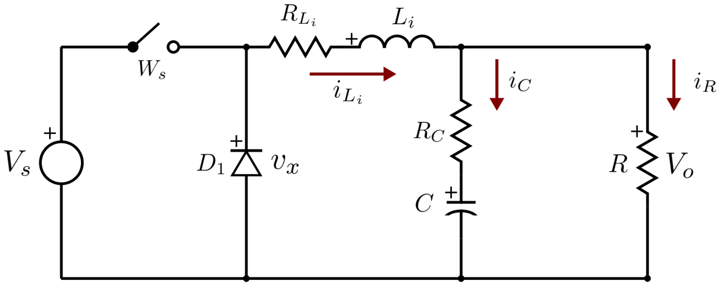
3. DC-DC Buck Converter Analysis

The DC-DC buck converter topology which considers the parasitic elements of the capacitor and inductor is shown in Figure 1. It consists of a DC input source V s , a controlled ideal switch W s , a rectifier diode D 1 , a filtering inductor L i , a filtering capacitor C, a load resistance R, and the equivalent series resistance (ESR) R c and R L i of the capacitor and the inductor, respectively.
The switched model [18] of the DC-DC buck converter in continuous conduction mode (CCM) shown in the Figure 1 is given by
v ˙ c i ˙ L i = γ R C γ C γ L i R c γ + R L i L i v c i L i + 0 V s L i u + ζ v ζ i , y = 1 0 v c i L i ,
where v c ( t ) is the capacitor voltage, i L i ( t ) is the inductor current, ζ v is a disturbance in the voltage capacitor, ζ i is a disturbance in the inductor current, u { 0 , 1 } is the control input, and γ = R R + R c .
For stability analysis and control purposes, this paper uses the large-signal-averaged model that provides a good representation of the system macroscopic behavior and allows to obtain the system response based on a continuous control input [46,47]. The large-signal averaged model based on the set of state Equation (10) is given by
v ˙ c ( t ) 0 = 1 C γ i L i ( t ) 0 v c ( t ) 0 R + ζ v , i ˙ L i ( t ) 0 = 1 L i V s 0 D c ( t ) γ v c ( t ) 0 ( γ R c + R L i ) i L i ( t ) 0 + ζ i ,
where 0 denotes an average of the states variables over the switching period, and D c is the duty cycle or continuous control input. Next, for simplicity, the brackets of averaged values are dropped. Thus the average dynamic Equation (11) can be written as
v ˙ c ( t ) = a 1 v c + a 2 i L i + ζ v i ˙ L ( t ) = a 3 v c + a 4 i L i + a 5 D c ( t ) + ζ i ,
where a 1 = γ R C , a 2 = γ C , a 3 = γ L i , a 4 = R c γ + R L i L i and a 5 = V s L i . From (12) the following model is obtained:
v ¨ c ( t ) a 2 a 5 v ˙ c ( t ) a 1 + a 4 a 2 a 5 v c ( t ) a 2 a 3 a 1 a 4 a 2 a 5 = D c ( t ) a 4 a 2 a 5 ζ v + 1 a 5 ζ i + 1 a 2 a 5 ζ ˙ v .
Let us define the output voltage error as
ϵ 1 ( t ) = v c ( t ) v r e f ,
where v r e f > 0 is constant and represents the desired output voltage. Therefore, the output tracking error dynamics of the system can be represented as a chain of integrators as
ϵ ˙ 1 ( t ) = ϵ 2 ( t ) ϵ ˙ 2 ( t ) = ϵ 1 ( t ) ( a 2 a 3 a 1 a 4 ) + ϵ 2 ( t ) ( a 1 + a 4 ) + a 2 a 5 D c ( t ) + ξ ( t ) x ¯ 0 ( t ) = ϵ 1 ( t ) + Δ ( t ) ,
where ξ ( t ) = a 2 ζ i a 4 ζ v + ζ ˙ v + v r e f ( a 2 a 3 a 1 a 4 ) represents a disturbance, and Δ ( t ) is the measurement noise.

4. Proposed Control Strategy

In this section, the following system is considered (15), where ξ ( t ) is considered such that ξ ξ ( t ) ξ + . Furthermore, Δ ( t ) at time t k satisfies Assumption 2. On the other hand, D c ( t ) is defined as
D c ( t ) = u k m a x i f u k u k m a x u k i f u k m i n < u k < u k m a x u k m i n i f u k u k m i n , t [ t k , t k + 1 ) , u k = K Z k , K = [ k i k p k d ] , Z k = [ z I , k z 0 , k z 1 , k ] T , z I , k = z I , k 1 + τ z 0 , k + z 0 , k 1 2 ,
where z I , k is an approximation of 0 t x 0 ( α ) d α . Although a trapezoidal integration is used in (16), it can be changed with other methods. In order to select an adequate gain, K , a discrete-time analysis is performed, then the discrete-time version of (15) is given as
X k + 1 = Φ ( τ ) X k + τ 3 4 τ 2 2 ! τ a 2 a 5 D c ( t k ) + ξ ( t k ) + τ 2 σ 0 , k + 1 + σ 0 , k 0 0 , X k = [ z I ( t k ) ϵ 1 , k ϵ 2 , k ] T , τ = t k + 1 t k ,
Φ ( τ ) = 1 τ + τ 3 4 a 2 a 3 a 1 a 4 τ 2 2 + τ 3 4 a 1 + a 4 0 1 + τ 2 2 a 2 a 3 a 1 a 4 τ + τ 2 2 a 1 + a 4 0 τ a 2 a 3 a 1 a 4 1 + τ a 1 + a 4 .
The above equation is obtained using Taylor series expansion for ϵ 1 ( t ) and ϵ 2 ( t ) . With the purpose of estimating the states ϵ 1 , k and ϵ 2 , k , one can modify the discrete-time differentiator (5) as follows:
w j f , k + 1 = τ ( n f j f + 1 ) ( n f j f + 1 ) ! ( z 0 , k x ¯ 0 , k ) + l = j f n f τ ( l j f ) ( l j f ) ! w l , k + l = j f n f + 2 τ ( l j f + 1 ) ( l j f + 1 ) ! ϕ l 1 , n f + 1 w 1 , k + 1 , z 0 , k + 1 = z 0 , k + τ z 1 , k + τ ϕ n f , n f + 1 w 1 , k + 1 + τ 2 2 ϕ n f + 1 , n f + 1 w 1 , k + 1 , z 1 , k + 1 = z 1 , k + τ ϕ n f + 1 , n f + 1 w 1 , k + 1 , j f = 1 , 2 , , n f .
where it is implemented using Lemma 1, L | ϵ 1 ( t k ) ( a 2 a 3 a 1 a 4 ) + ϵ 2 ( t k ) ( a 1 + a 4 ) + ξ ( t ) | , and z 0 , k and z 1 , k are estimations of ϵ 1 , k and ϵ 2 , k . The estimation errors of the discrete-time filtering observer (19) are defined as σ 0 , k = z 0 , k ϵ 1 , k and σ 1 , k = z 1 , k ϵ 2 , k . Additionally, without saturation of the control law (16), system (17) can be represented as follows:
X k + 1 = Ω τ X k + Θ k ( τ ) ,
where Ω τ and Θ k ( τ ) are defined as follows:
Ω τ = 1 + τ 3 4 a 2 a 5 k i τ + τ 3 4 a 2 a 3 a 1 a 4 + a 2 a 5 k p τ 2 2 + τ 3 4 a 1 + a 4 + a 2 a 5 k d τ 2 2 a 2 a 5 k i 1 + τ 2 2 a 2 a 3 a 1 a 4 + a 2 a 5 k p τ + τ 2 2 a 1 + a 4 + a 2 a 5 k d τ a 2 a 5 k i τ a 2 a 3 a 1 a 4 + a 2 a 5 k p 1 + τ a 1 + a 4 + a 2 a 5 k d , Θ k ( τ ) = τ 2 σ 0 , k + 1 + σ 0 , k + τ 3 4 ξ ( t k ) + a 2 a 5 E k τ 2 2 ! ξ ( t k ) + a 2 a 5 E k τ ξ ( t k ) + E k ,
with E k = k p σ 0 , k + k d σ 1 , k . Note that each element of matrix Θ k ( τ ) is bounded after a finite-time, and their bounds are defined by μ j parameters, which depend on λ j parameters and the methodology used to estimate ϵ j , k . Then, K is selected such that the magnitude of the n + 1 eigenvalues of Ω ( τ ) are lower than one and k i < 0 , k p < 0 and k d < 0 . Before presenting the following theorems, the following definitions are presented:
  • t k 0 is the lowest sampling time such that D c ( t ) is saturated for any measurement time greater than t k 0 and previous to the instant of time t k 2 , i.e., u k u k m a x or u k u k m i n for any t k with t k 0 t k < t k 2 .
  • t k 1 is the sampling time when the discrete-time filtering observer (19) obtains and keeps the accuracy (9).
  • t k 2 is the time instant such that u k is unsaturated and for the previous measurement time u k was saturated, i.e., u k m i n < u k < u k m a x at t k 2 , and u k u k m a x or u k u k m i n for any t k with t k 0 t k < t k 2 .
  • t k 3 is the sampling time when u k m a x > u k > u k m i n and the discrete-time filtering observer (19) obtains and keeps the accuracy (9).
  • u ¯ ( t ) is the continuous-time function analogous to u k , defined as
    u ¯ ( t ) = K z ¯ I ( t ) ϵ 1 ( t ) ϵ 2 ( t ) T , z ¯ I ( t ) = z I , k , for t [ t k , t k + 1 ) .
  • t f is the time instant after t k 0 and t k 1 such that u k m i n < u ¯ ( t f ) < u k m a x .
Time instants t k 0 , t k 1 , t k 2 and t k 3 are measurement times but t f may not be a measurement time. Now, the main results are presented:
Theorem 2.
Let system (15) under the controller D c ( t ) be defined as in (16) and using the implicit discrete-time filtering observer (19). K is selected such that the magnitude of the eigenvalues of Ω ( τ ) have a modulus lower than one and k I < 0 , k p < 0 , and k d < 0 if the following conditions are satisfied:
a 2 a 5 u k m a x > 4 τ 2 L 1 ( a 2 a 3 a 1 a 4 ) L 1 + 2 τ L 2 a 1 + a 4 L 2 + + 4 μ 0 L ρ 2 τ 2 ξ k , a 2 a 5 u k m i n < 4 τ 2 L 1 + ( a 2 a 3 a 1 a 4 ) L 1 2 τ L 2 + a 1 + a 4 L 2 4 μ 0 L ρ 2 τ 2 ξ k + ,
u k m i n u k or u k u k m a x at the time instant t k 1 , | σ 0 , k | , | σ 1 , k | , and τ are such that
k i z I , k + k p L 1 + k d L 2 + | E k | < u k m a x , k i z I , k + k p L 1 + + k d L 2 + | E k | > u k m i n ,
with E k at time t k 2 , then u k m i n < u k < u k m a x at time t k 2 .
Proof. 
Considering the case u k u k m a x at time t k 1 . If t k 2 t t k 0 , then ϵ 1 ( t ) and ϵ 2 ( t ) are defined as
ϵ 1 ( t ) = F 1 ( t ) + G 1 ( t ) , ϵ 2 ( t ) = F 2 ( t ) + G 2 ( t ) ,
where F 1 ( t ) , F 2 ( t ) , G 1 ( t ) and G 2 ( t ) are given as:
F 1 ( t ) = L 1 s 2 ( a 1 + a 4 ) s ϵ 1 ( 0 ) + s ϵ 2 ( 0 ) + a 2 a 5 u k m a x s s 2 ( a 1 + a 4 ) s ( a 2 a 3 a 1 a 4 ) , F 2 ( t ) = L 1 a 1 + a 4 ϵ 1 ( 0 ) + s ϵ 2 ( 0 ) + a 2 a 5 u k m a x s 2 ( a 1 + a 4 ) s ( a 2 a 3 a 1 a 4 ) , G 1 ( t ) = L 1 L ξ ( t ) s 2 ( a 1 + a 4 ) s ( a 2 a 3 a 1 a 4 ) , G 2 ( t ) = L 1 L ξ ( t ) s s 2 ( a 1 + a 4 ) s ( a 2 a 3 a 1 a 4 ) .
which depend on the roots r 1 = a 1 + a 4 + a 1 + a 4 2 + 4 ( a 2 a 3 a 1 a 4 ) 2 and r 2 = a 1 + a 4 a 1 + a 4 2 + 4 ( a 2 a 3 a 1 a 4 ) 2 , whose real part is negative. Here, L · is the Laplace transform. Therefore, F 1 ( t ) and F 2 ( t ) are continuous functions such that
lim t F 1 ( t ) = a 2 a 5 u k m a x ( a 2 a 3 a 1 a 4 ) , lim t F 2 ( t ) = 0 .
Let L 1 + , L 1 , L 2 + and L 2 such that L 1 ϵ 1 ( t ) L 1 + , L 2 ϵ 2 ( t ) L 2 + , for any t t k 1 . One can rewrite z I , k + 1 z I , k
z I , k + 1 z I , k τ L 1 + τ 3 4 a 2 a 3 a 1 a 4 L 1 + + τ 2 2 L 2 + τ 3 4 a 1 + a 4 L 2 + + + τ 3 4 a 2 a 5 u k m a x + ξ k τ μ 0 L ρ 2 , z I , k + 1 z I , k τ L 1 + + τ 3 4 a 2 a 3 a 1 a 4 L 1 + τ 2 2 L 2 + + τ 3 4 a 1 + a 4 L 2 + + τ 3 4 a 2 a 5 u k m a x + ξ k + + τ μ 0 L ρ 2 ,
Since a 2 a 5 u k m a x > 4 τ 2 L 1 ( a 2 a 3 a 1 a 4 ) L 1 + 2 τ L 2 a 1 + a 4 L 2 + + 4 μ 0 L ρ 2 τ 2 ξ k then z i , k is increasing. Due to the above fact and the limits (27), u ¯ ( t ) will satisfy the condition
u ¯ ( t f ) < u k m a x
at the instant of time t f . Now, it is considered the value of u k for the sampling time after t f , which was defined as t k 2 . The estimation errors | σ 0 , k | , | σ 1 , k | and sampling time τ must be small enough to satisfy the following condition:
u k m a x > u ¯ ( t k 2 ) + E k > u k m i n .
where E k is defined at time t k 2 and t f + τ t k 2 t f . The above condition implies that u k is unsaturated at the sampling time t k 2 . Furthermore, the above condition can be satisfied if
k i z I , k + k p L 1 + k d L 2 + | E k | < u k m a x , k i z I , k + k p L 1 + + k d L 2 + | E k | > u k m i n ,
are satisfied, where z I , k is defined at the sampling time t k 2 . A similar demonstration can be performed for the case u k u k m i n at the sampling time t k 1 , where F 1 ( t ) and F 2 ( t ) are defined with u k m i n instead of u k m a x , with the following condition:
a 2 a 5 u k m i n < 4 τ 2 L 1 + ( a 2 a 3 a 1 a 4 ) L 1 2 τ L 2 + a 1 + a 4 L 2 4 μ 0 L ρ 2 τ 2 ξ k + .
It concludes the proof. □
Theorem 2 shows that after the discrete-time differentiator (5) obtains the asymptotic accuracy and if D c ( t ) is saturated at time t k 1 , then D c ( t ) is unsaturated at the sampling time t k 2 . The following step is to obtain the required conditions to keep D c ( t ) unsaturated and the system (17) stable. These conditions are presented in the following theorem:
Theorem 3.
Let system (15) be implemented with the control law D c ( t ) defined as in (16), where K is selected as in Theorem 2. If u k m i n u k u k m a x at the sampling time t k 3 , u k m a x and u k m i n satisfy the following conditions,
u k m a x > λ m a x ( P Ω ( τ ) Ω ( τ ) T P ) + λ m a x ( P ) λ m i n ( Q ) 1 Θ k 2 | k i + k d + k p | , u k m a x > K Ω i ( τ ) X k 3 + j = 0 i 1 K Ω j ( τ ) Θ k 3 + i j 1 , u k m i n < K Ω i ( τ ) X k 3 + j = 0 i 1 K Ω j ( τ ) Θ k 3 + i j 1 .
then discrete-time system (17) is stable, and D c ( t ) is unsaturated for any t k t k 3 .
Proof. 
A discrete-time Lyapunov function is proposed as
V k = X k T P X k ,
where P is a symmetric definite positive matrix. From the previous function, one obtains:
V k + 1 V k = X k T Ω ( τ ) T P Ω ( τ ) P X k + 2 X k T Ω ( τ ) T P Θ k ( τ ) + Θ k ( τ ) T P Θ k ( τ ) , V k + 1 V k X k T Q X k + X k T X k + Θ k ( τ ) T P Ω ( τ ) Ω ( τ ) T P + P Θ k ( τ ) , V k + 1 V k λ m i n ( Q ) 1 X k 2 2 + λ m a x ( P Ω ( τ ) Ω ( τ ) T P ) + λ m a x ( P ) Θ k ( τ ) 2 2 .
It implies that V k + 1 V k is negative if
X k 2 λ m a x ( P Ω ( τ ) Ω ( τ ) T P ) + λ m a x ( P ) λ m i n ( Q ) 1 Θ k ( τ ) 2 .
The above equation allows to define the convergence region of the discrete-time system and therefore, to keep an unsaturated control law. u k m a x must satisfy at least the following condition:
u k m a x > λ m a x ( P Ω ( τ ) Ω ( τ ) T P ) + λ m a x ( P ) λ m i n ( Q ) 1 Θ k 2 | k i + k d + k p |
Alternatively, one can obtain the following inequality:
V k + 1 V k X k T Ω ( τ ) T P Ω ( τ ) P + Ω T P Λ P Ω X k + Θ k ( τ ) T Λ 1 + P Θ k ( τ ) ,
where Λ is a positive definite matrix and Q is defined as Q = Ω ( τ ) T P Ω ( τ ) + P Ω T P Λ P Ω . Then, one obtains
V k + 1 V k X k T Q ( τ ) X k + Θ k ( τ ) T Λ 1 + P Θ k ( τ ) ,
Then, if there exists positive definite matrices P , Q , Λ with P = P T , the following conditions can be presented:
X k 2 λ m a x ( Λ 1 + P ) λ m i n ( Q ) Θ k ( τ ) 2 , u k m a x λ m a x ( Λ 1 + P ) λ m i n ( Q ) Θ k ( τ ) 2 k i + k p + k d .
Without saturation, the solution of the discrete-time system (20) is given as
X k 3 + i = Ω i ( τ ) X k 3 + j = 0 i 1 Ω j ( τ ) Θ k 3 + i j 1 ( τ ) ,
with i = 1 , 2 , 3 , . The above allows to define u k 3 as
u k 3 + i = K Ω i ( τ ) X k 3 + j = 0 i 1 K Ω j ( τ ) Θ k 3 + i j 1 ( τ ) .
Then to keep an unsaturated control law D c ( t ) , u k m a x and u k m i n have to satisfy the following conditions:
u k m a x > K Ω i ( τ ) X k 3 + j = 0 i 1 K Ω j ( τ ) Θ k 3 + i j 1 ( τ ) , u k m i n < K Ω i ( τ ) X k 3 + j = 0 i 1 K Ω j ( τ ) Θ k 3 + i j 1 ( τ ) .
This concludes the proof. □
The conditions related to u k m a x and u k m i n in Theorem 3 define the convergence region of the discrete-time system, and they are given in Equation (36). Theorems 2 and 3 allow to show the stability of the continuous-time system (15) using the discrete-time law control (16). However, an sufficiently small sampling time is required. It is important to note that there are not values of u k m a x and u k m i n such that the discrete-time system is stable for any initial condition X k 3 , which comes from the conditions in Theorem 2. In order to clarify the use of the above theorems, we present the following numeric example:

Numeric Example

This example show how to calculate the conditions obtained from Theorem 3. Here, the parameters shown in Table 1 are used:
Equation (44) allows to calculate Ω ( τ ) , which is given as
Ω τ = 0.999999 0.0000249 3.06 10 10 0.046621 0.9959002 2.44899 10 5 3729.654194 327.9844193 0.959194 ,
and Θ k ( τ ) 2 0.047114 . Assuming that there exist Q 0 , P 0 , Λ 0 then the V k + 1 V k is negative if X k 2 such that
X k 2 λ m a x ( Λ 1 + P ) λ m i n ( Q ) Θ k ( τ ) 2 .
On the other hand, to keep the control unsaturated, X k 3 should satisfy the following conditions:
0.99 > 3 z ^ I , k 0.185 ϵ ^ 1 , k 0.00002 ϵ ^ 2 , k , 0.99 + 2.18909 10 7 > 2.91678 z ^ I , k 0.17775 ϵ ^ 1 , k 0.0000237 ϵ ^ 2 , k , 0.99 1.694679 10 7 > 2.82004 z ^ I , k 0.169322 ϵ ^ 1 , k 0.0000271 ϵ ^ 2 , k , 0.99 5.169639 10 7 > 2.711065 z ^ I , k 0.15981 ϵ ^ 1 , k 0.00003014 ϵ ^ 2 , k ,
0.01 < 3 z ^ I , k 0.185 ϵ ^ 1 , k 0.00002 ϵ ^ 2 , k , 0.01 + 2.18909 10 7 < 2.91678 z ^ I , k 0.17775 ϵ ^ 1 , k 0.0000237 ϵ ^ 2 , k , 0.01 1.694679 10 7 < 2.82004 z ^ I , k 0.169322 ϵ ^ 1 , k 0.0000271 ϵ ^ 2 , k , 0.01 5.169639 10 7 < 2.711065 z ^ I , k 0.15981 ϵ ^ 1 , k 0.00003014 ϵ ^ 2 , k ,
where X k 3 = [ z ^ I , k ϵ ^ 1 , k ϵ ^ 2 , k ] T , and the value of Θ k ( τ ) was selected as a random value between its maximum and minimum values, which are given as
Θ M k ( τ ) = 1.882362 10 9 5.889251 10 7 0.047114 , Θ m k ( τ ) = 1.882362 10 9 5.889251 10 7 0.047114 .
Therefore, for any X k 3 such that satisfy the above conditions define the stability area of the system.

5. Experimental Results

This section evaluates the performance of the proposed control strategy through experimentation. The block diagram of the entire system is shown in Figure 2. The system is divided into three sections: the DC-DC buck converter, the digital control device, and the peripheral signal conditioning subsystems (anti-aliasing filter and MOSFET drivers).

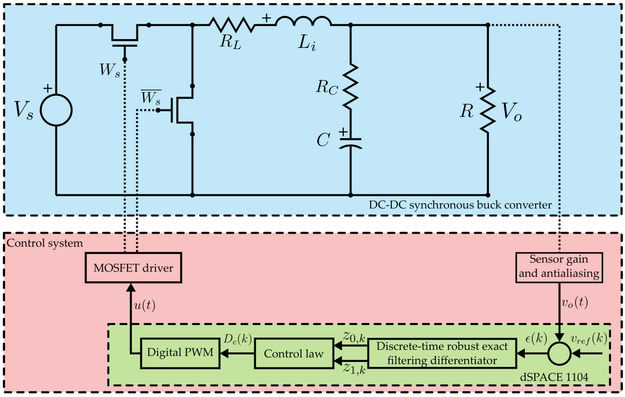
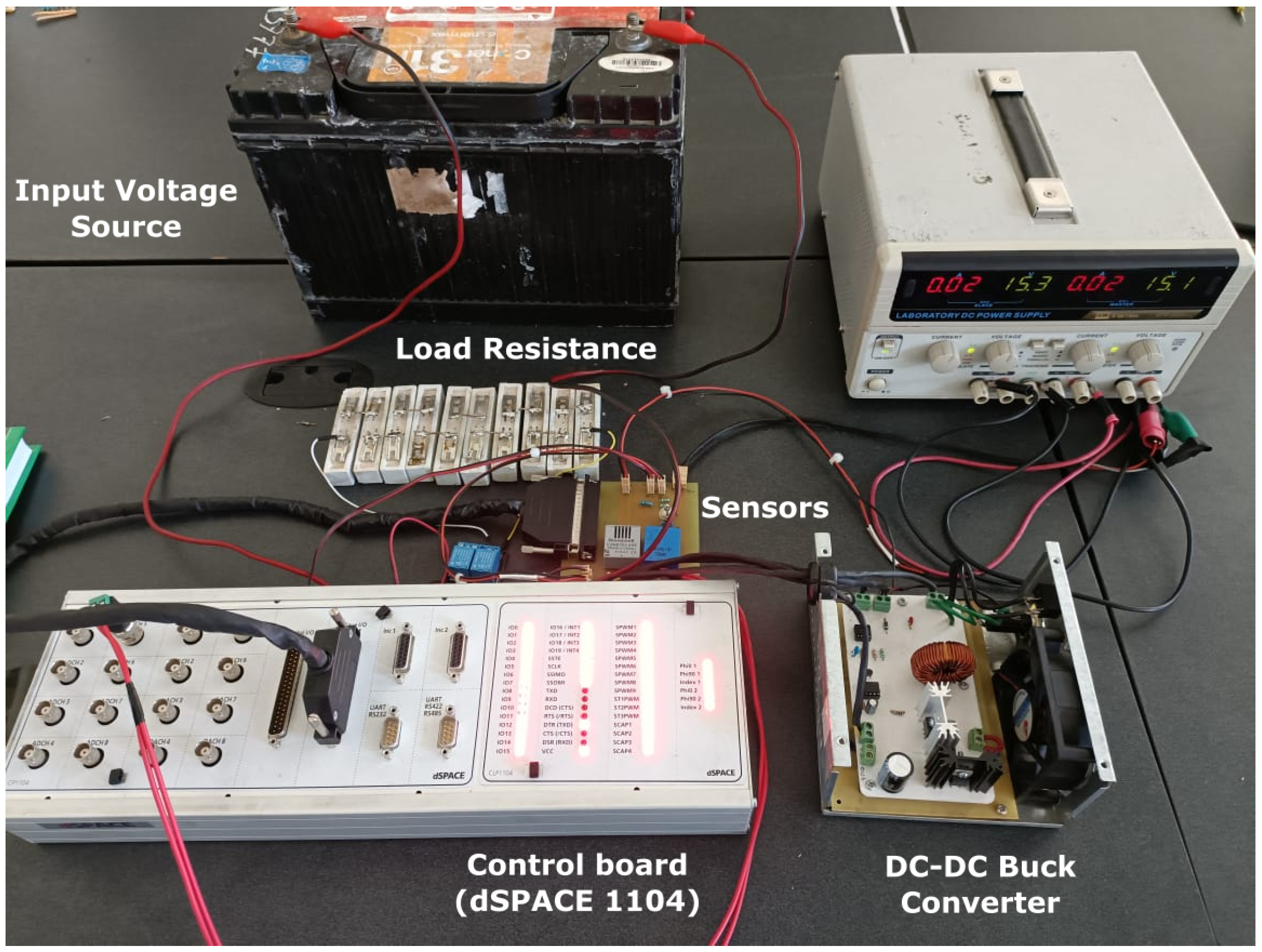
5.1. System Implementation

For the control algorithm validation, a prototype of the DC-DC buck converter with synchronous rectification was designed and built with the parameters shown in the Table 2. The design of the DC-DC buck converter corresponds to an output voltage variation due to a capacitor less than 2% and an inductor current ripple less than 40% [48,49,50]. The converter operates in CCM for the entire range of values specified in Table 2 [51].
The proposed control law (16) is implemented based on the robust exact filtering differentiator (19) with a differentiation order n = 1 and a filter order n f = 1 . It is given as
w 1 , k + 1 = w 1 , k + τ z 0 , k ϵ 1 , k τ λ 2 L 1 3 | w 1 , k + 1 | 2 3 ξ k τ 2 2 λ 1 L 2 3 | w 1 , k + 1 | 1 3 ξ k τ 3 6 λ 0 L ξ k , z 0 , k + 1 = z 0 , k + τ z 1 , k τ λ 1 L 2 3 | w 1 , k + 1 | 1 3 ξ k τ 2 2 λ 0 L ξ k , z 1 , k + 1 = z 1 , k τ λ 0 L ξ k ,
Lemma 1 is used to calculate w 1 , k + 1 on the right hand of (49), with the methodology presented in [45] and two iterations of Halley’s method to estimate the polynomials roots given as
p r = r 3 + a 2 r 2 + a 1 r + b k + a 0 , p r = r 3 + a 2 r 2 + a 1 r + b k + a 0 ,
where a 0 = τ 3 6 λ 0 L , a 1 = τ 2 2 λ 1 L 2 3 , a 2 = τ λ 2 L 1 3 and b k = w 1 , k τ z 0 , k ϵ 1 , k .
The digital platform selected to execute the algorithm is the dSPACE DS1104 R&D Controller Board, with a voltage feedback loop sampled at two different frequencies for comparison purposes. A 16-bit resolution is used for analog-to-digital conversion, and the resolution of the digital pulse-width modulator (DPWM) is 50 ns. Serial communication between the dSPACE platform and ControlDesk software is used to monitor the DC-DC buck converter output voltage V o ( t k ) , duty cycle D c ( t k ) and the system error ϵ 1 ( t k ) .
In order to avoid frequency distortion in the voltage control loop due to the aliasing effect, a second-order Chebyshev low-pass filter with −20 dB of attenuation gain at the Nyquist frequency is used. The analog filter implementation is performed through a non-inverting Sallen–Key topology with the op-amp OPA4187. Finally, the DC-DC synchronous buck converter switches are ultra-low on-resistance power MOSFET IRF3710 driven via dual low side driver IR4427 to minimize propagation times and a pair of 6N135 high-speed photocoupler to isolate the control signal from the power section.

5.2. Experimental Results

The experiments shown in this section and their corresponding subsections use the control parameters of Table 3, where K is selected according to the Theorem 2, hence, eigenvalues of Ω ( τ ) are 0.9995 , 0.9554 + 0.0974 i and 0.9554 0.0974 i for τ = 25 μ s and 0.9956 , 0.2943 + 0.8080 i and 0.9956 0.8080 i for τ = 250 μ s (calculated using the maximum values of Table 2). Finally, λ j is properly selected according to [52]. Likewise, Figure 3 shows the physical prototype of the system. Experiments are performed with different values of load resistance and supply voltage to ensure that the controller is robust enough to handle these uncertainties.
Additionally, the proposed state feedback controller is compared with a saturated discrete-time PID controller with filter in the derivative action given as
D c ( t ) = u k m a x i f u k u k m a x u k i f u k m i n < u k < u k m a x u k m i n i f u k u k m i n , u k = Z 1 [ E ( z ) G ( z ) ] , G ( z ) = k p p i d f + k i p i d f τ 2 z + 1 z 1 + k d p i d f f n 1 + f n τ z z 1 ,
with k p p i d f = 0.1 , k i p i d f = 1.5 , k d p i d f = 0.00002 and f n = 150 . Here Z 1 · is the inverse Z transform.

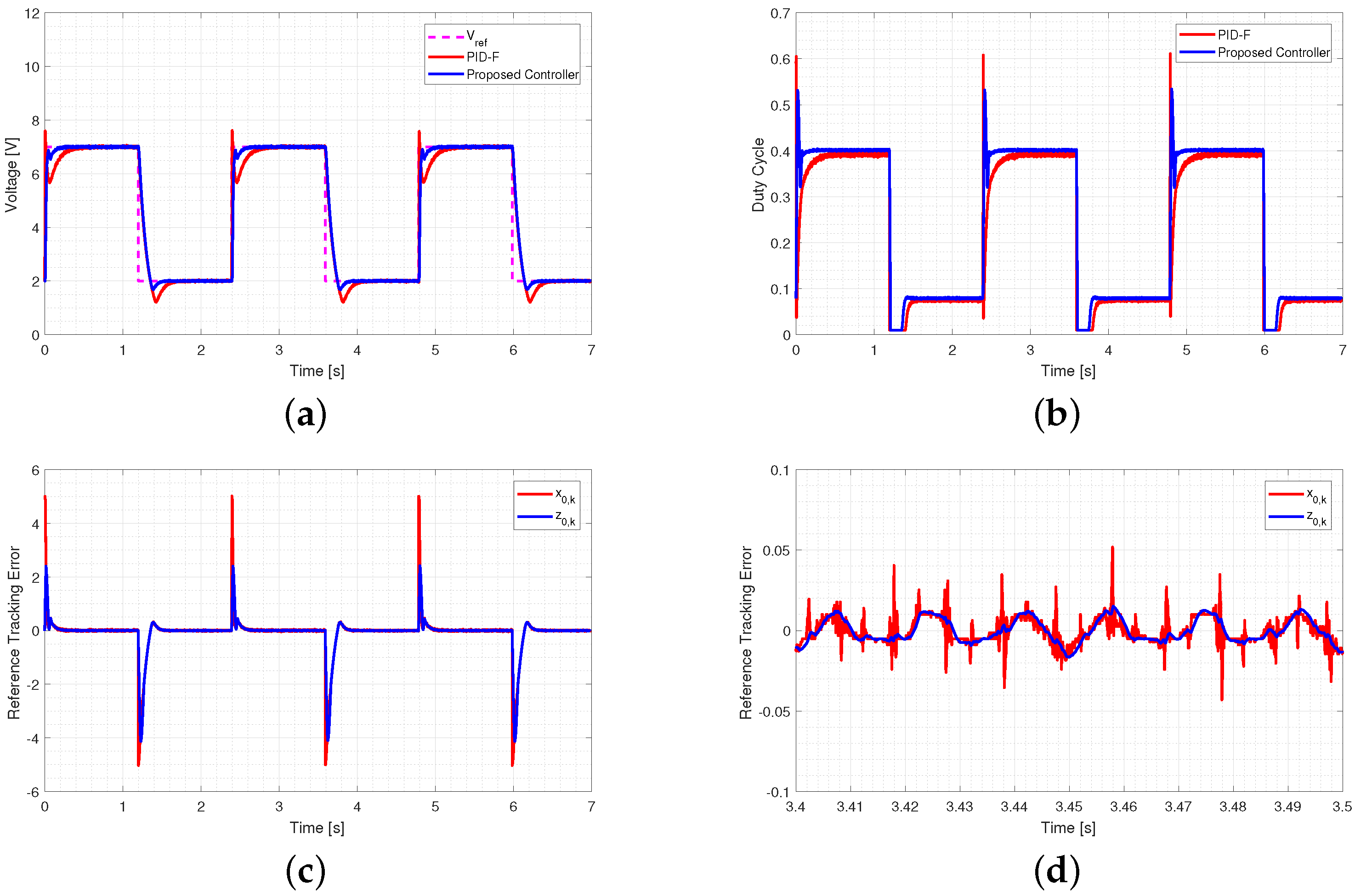
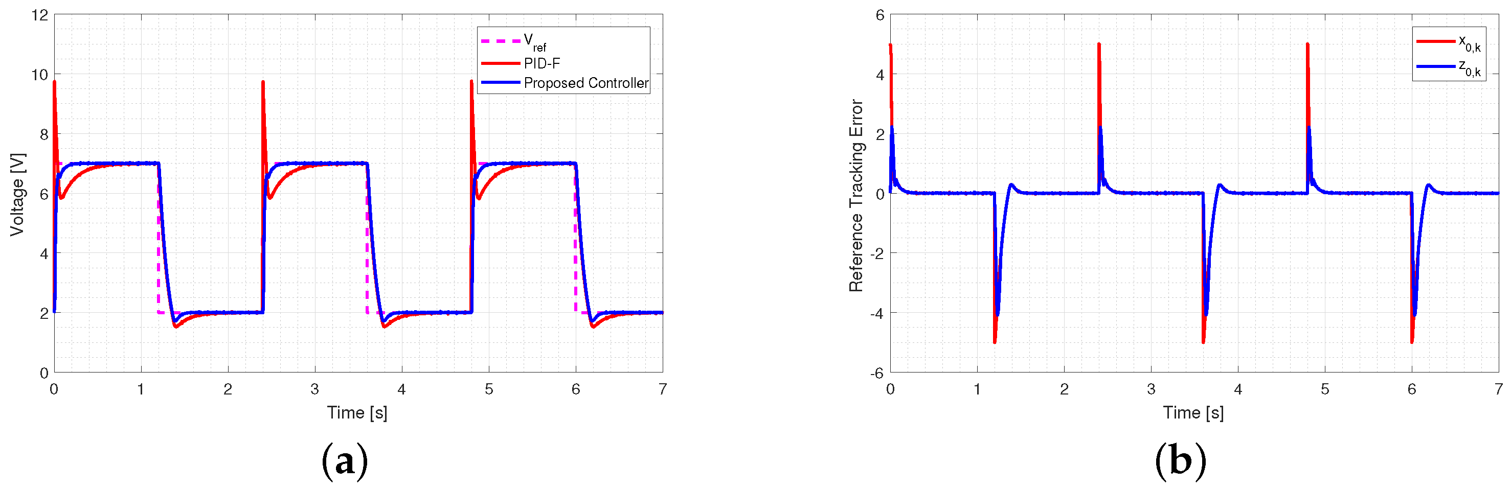
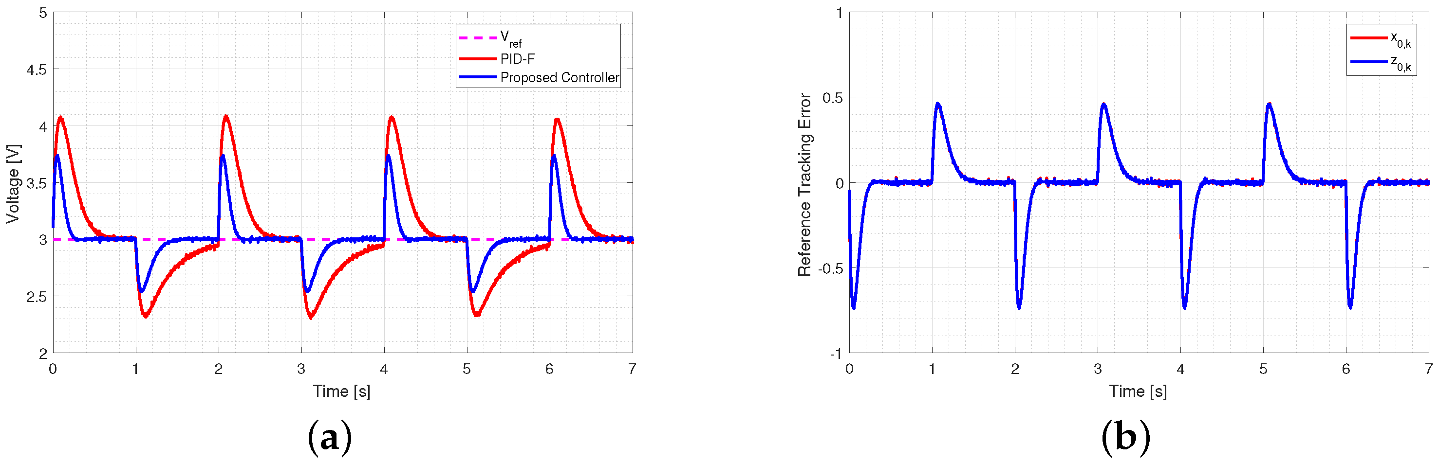
5.2.1. Output Voltage Tracking Performance

This analysis considers that the desired output voltage suddenly changes between V r e f , t 1 = 2 V and V r e f , t 2 = 7 V. The experiments being shown in this subsection use a fixed supply voltage of V s = 12.7 V and a constant load of R = 120 Ω . This operating point is selected because the value of R produces that the current in the inductor decreases almost to zero (discontinuous conduction mode DCM). Figure 4 shows the results of output voltage tracking performance for τ = 25 μ s and Figure 5 for τ = 250 μ s. Notice that the proposed controller behaves better during reference changes since the settling time and percent overshoot are small enough. Additionally, it is noted that the proposed controller enters the saturation region of u k m i n ; however, the voltage tracking is done correctly.

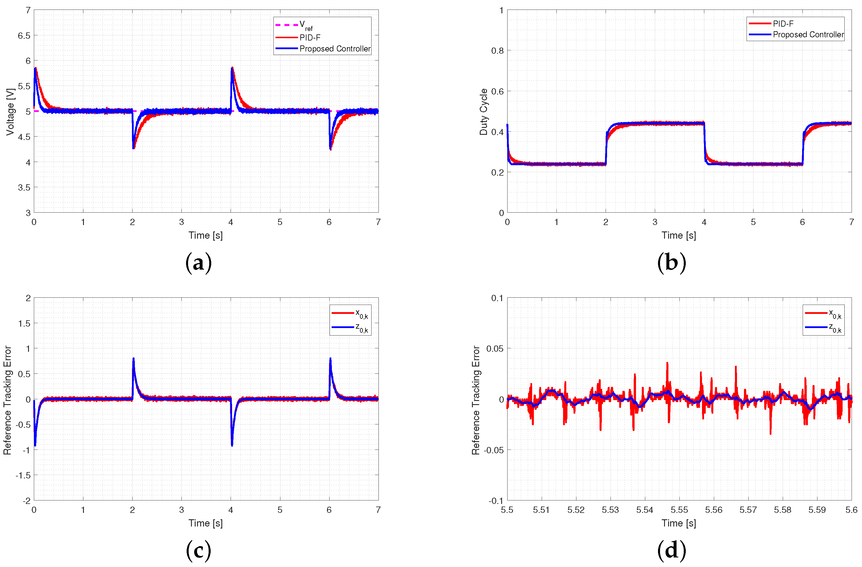
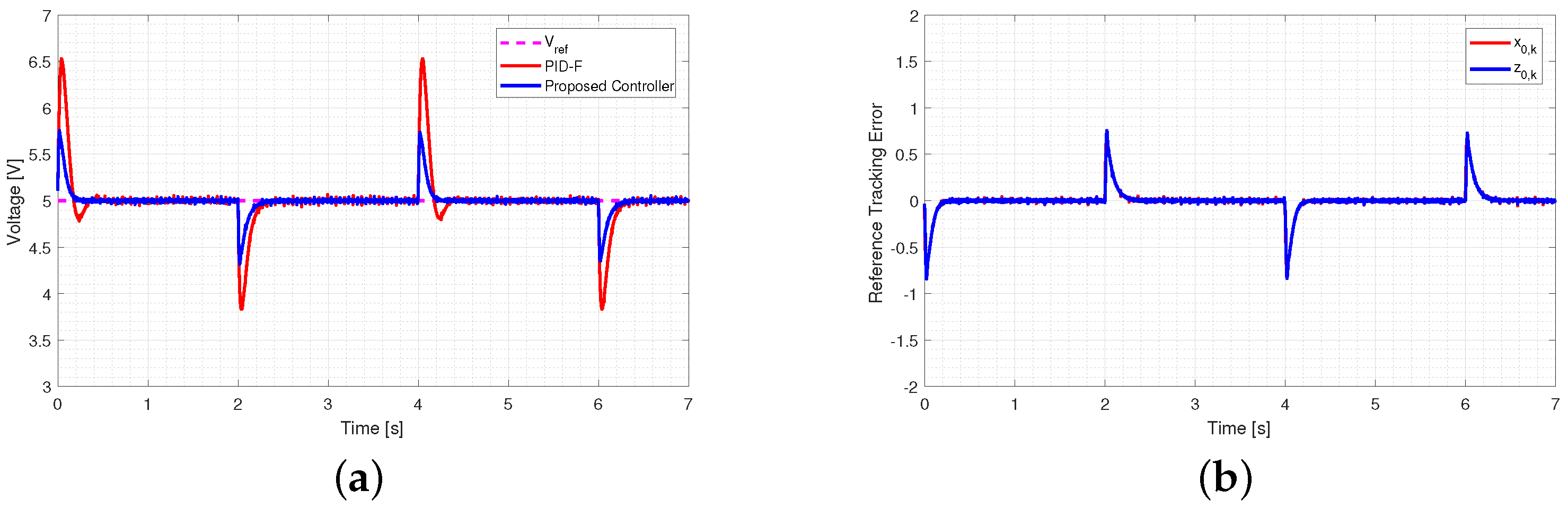
5.2.2. Load Variation Performance

This analysis shows the controller’s behavior in response to load disturbances, a typical situation in power electronic converters. The experiments in this subsection are performed with V s = 12.7 , V r e f = 5 V, and the load resistance that changes every 2 s between the values R t 1 = 120 Ω and R t 2 = 40 Ω . The result of output voltage regulation under these conditions is shown in Figure 6 for τ = 25 μ s and Figure 7 for τ = 250 μ s. It is observed that the controller can suppress these disturbances, while the state estimation does not diverge from the real value during the transient state. Note that the response of the discrete-time PID controller is worse when implemented at a lower frequency.

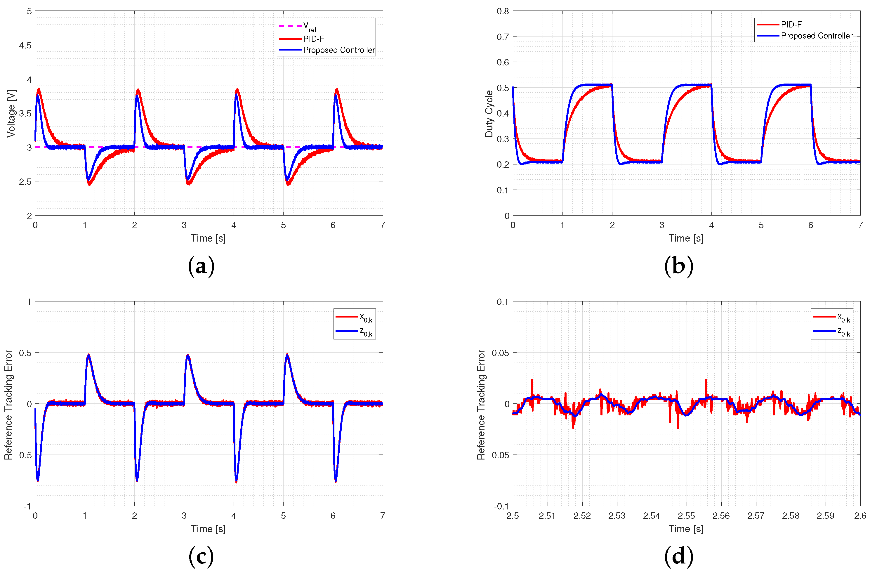
5.2.3. Input Voltage Variation

In this experiment, the input voltage of the DC-DC buck converter varies instantaneously between two values every second. The parameters of the experiments in this subsection are the supply voltage that changes between the values V s t 1 = 6 V and V s t 2 = 10 V and R = 120 Ω . Figure 8 shows the results of the experiment for τ = 25 μ s and Figure 9 for τ = 250 μ s. It is possible to see that the estimation of the system error z 0 , k presents a considerably smaller noise amplitude than the system state x 0 , k , even when the robust exact time filtering differentiator is implemented at a lower frequency.

6. Conclusions

This paper presents a new digital controller for a DC-DC buck converter with duty cycle saturation. The proposed structure relies on a robust exact filtering differentiator based on the implicit discretization of the homogeneous differentiator. Additionally, the design considers the physical constraints of the DC-DC buck converter by adding a saturation law. Moreover, the conditions for preserving the asymptotic precision of the robust exact time differentiator are given, and the convergence analysis of the discrete-time system. Likewise, these theorems offer a guide for selecting the control gains K .
The main advantage of this control scheme lies in the relationship between the estimation accuracy of the system states and noise filtration performances. This feature is especially useful in systems whose composition is based on switching actuators subject to high-frequency noise, as in the DC-DC buck converter. Likewise, the problem of filtering a noisy signal is often addressed, which is essential for implementing a derivative through discrete time. Real-time experimentation was carried out based on an efficient implementation method of the implicit discrete-time differentiator to ensure the effectiveness of the proposed control law, where the output voltage tracking performance and robustness to load and supply voltage variations were analyzed.
The results show a satisfactory performance and a sufficiently accurate estimation of the error, even in the presence of disturbances and measurement noise for a sampling period of τ = 25 μ s and τ = 250 μ s, with a minimum difference in the measurement noise filtering capacity. Likewise, the proposed controller showed a better behavior than a saturated discrete-time PID with a filter in the derivative action, primarily when implemented at a lower frequency. This feature is desirable for practical control applications where hardware resources and digital processing capabilities are limited, and the plant is subject to measurement noise.

Author Contributions

Conceptualization, M.A.A.-C., J.D.S.-T. and G.J.R.-A.; methodology, J.E.C.-R.; software, M.A.A.-C. and J.E.C.-R.; validation, J.D.S.-T., G.J.R.-A. and D.E.C.-P.; formal analysis, J.E.C.-R.; investigation, M.A.A.-C. and J.E.C.-R.; resources, D.E.C.-P.; data curation, M.A.A.-C.; writing—original draft preparation, M.A.A.-C. and J.E.C.-R.; writing—review and editing, J.D.S.-T.; visualization, G.J.R.-A. and D.E.C.-P.; supervision, G.J.R.-A. and D.E.C.-P.; project administration, G.J.R.-A. All authors have read and agreed to the published version of the manuscript.

Funding

This research received no external funding.

Institutional Review Board Statement

Not applicable.

Informed Consent Statement

Not applicable.

Data Availability Statement

Not applicable.

Acknowledgments

The authors appreciate the support of Consejo Nacional de Ciencia y Tecnológia (CONACYT) and Tecnológico Nacional de México (TecNM).

Conflicts of Interest

The authors declare no potential conflict of interest.

Abbreviations

The following abbreviations are used in this manuscript:
UPSUninterruptible power supply
GPIGeneralized proportional integral
PIDProportional integral derivative
FPGAField-programmable gate array
DSPDigital signal processor
SMSliding mode
PIAWProportional integral with anti-windup
ESREquivalent series resistance
CCMContinuous conduction mode
DPWMDigital pulse-width modulator
DCMDiscontinuous conduction mode

References

  1. Goyal, V.K.; Shukla, A. Isolated DC–DC Boost Converter for Wide Input Voltage Range and Wide Load Range Applications. IEEE Trans. Ind. Electron. 2021, 68, 9527–9539. [Google Scholar] [CrossRef]
  2. Wai, R.J.; Lin, C.Y.; Duan, R.Y.; Chang, Y.R. High-Efficiency DC-DC Converter with High Voltage Gain and Reduced Switch Stress. IEEE Trans. Ind. Electron. 2007, 54, 354–364. [Google Scholar] [CrossRef]
  3. Naayagi, R.T.; Forsyth, A.J.; Shuttleworth, R. High-Power Bidirectional DC–DC Converter for Aerospace Applications. IEEE Trans. Power Electron. 2012, 27, 4366–4379. [Google Scholar] [CrossRef]
  4. Nagata, H.; Uno, M. Nonisolated PWM Three-Port Converter Realizing Reduced Circuit Volume for Satellite Electrical Power Systems. IEEE Trans. Aerosp. Electron. Syst. 2020, 56, 3394–3408. [Google Scholar] [CrossRef]
  5. Dusmez, S.; Hasanzadeh, A.; Khaligh, A. Comparative Analysis of Bidirectional Three-Level DC–DC Converter for Automotive Applications. IEEE Trans. Ind. Electron. 2015, 62, 3305–3315. [Google Scholar] [CrossRef]
  6. Park, J.; Choi, S. Design and Control of a Bidirectional Resonant DC–DC Converter for Automotive Engine/Battery Hybrid Power Generators. IEEE Trans. Power Electron. 2014, 29, 3748–3757. [Google Scholar] [CrossRef]
  7. Turksoy, A.; Teke, A.; Alkaya, A. A comprehensive overview of the dc-dc converter-based battery charge balancing methods in electric vehicles. Renew. Sustain. Energy Rev. 2020, 133, 110274. [Google Scholar] [CrossRef]
  8. Sivamani, D.; Ramkumar, R.; Nazar Ali, A.; Shyam, D. Design and implementation of highly efficient UPS charging system with single stage power factor correction using SEPIC converter. Mater. Today Proc. 2021, 45, 1809–1819. [Google Scholar] [CrossRef]
  9. Zhan, Y.; Guo, Y.; Zhu, J.; Wang, H. Intelligent uninterruptible power supply system with back-up fuel cell/battery hybrid power source. J. Power Sources 2008, 179, 745–753. [Google Scholar] [CrossRef] [Green Version]
  10. Hong, T.; Geng, Z.; Qi, K.; Zhao, X.; Ambrosio, J.; Gu, D. A Wide Range Unidirectional Isolated DC-DC Converter for Fuel Cell Electric Vehicles. IEEE Trans. Ind. Electron. 2021, 68, 5932–5943. [Google Scholar] [CrossRef]
  11. Kwon, J.M.; Kim, E.H.; Kwon, B.H.; Nam, K.H. High-Efficiency Fuel Cell Power Conditioning System with Input Current Ripple Reduction. IEEE Trans. Ind. Electron. 2009, 56, 826–834. [Google Scholar] [CrossRef]
  12. Oh, Y.G.; Choi, W.Y.; Kwon, J.M. Design of a Step-Up DC-DC Converter for Standalone Photovoltaic Systems with Battery Energy Storages. Energies 2022, 15, 44. [Google Scholar] [CrossRef]
  13. Bereš, M.; Kováč, D.; Vince, T.; Kováčová, I.; Molnár, J.; Tomčíková, I.; Dziak, J.; Jacko, P.; Fecko, B.; Gans, Š. Efficiency Enhancement of Non-Isolated DC-DC Interleaved Buck Converter for Renewable Energy Sources. Energies 2021, 14, 4127. [Google Scholar] [CrossRef]
  14. Pereira, A.V.C.; Cavalcanti, M.C.; Azevedo, G.M.; Bradaschia, F.; Neto, R.C.; Carvalho, M.R.S.d. A Novel Single-Switch High Step-Up DC–DC Converter with Three-Winding Coupled Inductor. Energies 2021, 14, 6288. [Google Scholar] [CrossRef]
  15. Qi, Q.; Ghaderi, D.; Guerrero, J.M. Sliding mode controller-based switched-capacitor-based high DC gain and low voltage stress DC-DC boost converter for photovoltaic applications. Int. J. Electr. Power Energy Syst. 2021, 125, 106496. [Google Scholar] [CrossRef]
  16. Zhu, B.; Liu, S.; Huang, Y.; Tan, C. Non-isolated high step-up DC/DC converter based on a high degrees of freedom voltage gain cell. IET Power Electron. 2017, 10, 2023–2033. [Google Scholar] [CrossRef]
  17. Park, K.; Chen, Z. Control and dynamic analysis of a parallel-connected single active bridge DC–DC converter for DC-grid wind farm application. IET Power Electron. 2015, 8, 665–671. [Google Scholar] [CrossRef]
  18. Bacha, S.; Munteanu, I.; Bratcu, A.I. Power electronic converters modeling and control. Adv. Textb. Control. Signal Process. 2014, 454, 454. [Google Scholar]
  19. García-Alarcón, O.; Moreno-Valenzuela, J. Analysis and Design of a Controller for an Input-Saturated DC–DC Buck Power Converter. IEEE Access 2019, 7, 54261–54272. [Google Scholar] [CrossRef]
  20. Mazumder, S. Stability analysis of parallel DC-DC converters. IEEE Trans. Aerosp. Electron. Syst. 2006, 42, 50–69. [Google Scholar] [CrossRef]
  21. Zurita-Bustamante, E.W.; Linares-Flores, J.; Guzman-Ramirez, E.; Sira-Ramirez, H. A Comparison Between the GPI and PID Controllers for the Stabilization of a DC–DC “Buck” Converter: A Field Programmable Gate Array Implementation. IEEE Trans. Ind. Electron. 2011, 58, 5251–5262. [Google Scholar] [CrossRef]
  22. Seo, S.W.; Choi, H.H. Digital Implementation of Fractional Order PID-Type Controller for Boost DC–DC Converter. IEEE Access 2019, 7, 142652–142662. [Google Scholar] [CrossRef]
  23. NI, Y.; XU, J. Study of Discrete Global-Sliding Mode Control for Switching DC-DC Converter. J. Circuits Syst. Comput. 2011, 20, 1197–1209. [Google Scholar] [CrossRef]
  24. Seguel, J.L.; Seleme, S.I. Robust Digital Control Strategy Based on Fuzzy Logic for a Solar Charger of VRLA Batteries. Energies 2021, 14, 1001. [Google Scholar] [CrossRef]
  25. Wang, J.; Zhang, C.; Li, S.; Yang, J.; Li, Q. Finite-Time Output Feedback Control for PWM-Based DC–DC Buck Power Converters of Current Sensorless Mode. IEEE Trans. Control. Syst. Technol. 2017, 25, 1359–1371. [Google Scholar] [CrossRef]
  26. Aguilar-Ibanez, C.; Moreno-Valenzuela, J.; García-Alarcón, O.; Martinez-Lopez, M.; Acosta, J.A.; Suarez-Castanon, M.S. PI-Type Controllers and Σ − Δ Modulation for Saturated DC-DC Buck Power Converters. IEEE Access 2021, 9, 20346–20357. [Google Scholar] [CrossRef]
  27. Benzaouia, A.; Soliman, H.M.; Saleem, A. Regional pole placement with saturated control for DC-DC buck converter through Hardware-in-the-Loop. Trans. Inst. Meas. Control. 2016, 38, 1041–1052. [Google Scholar] [CrossRef]
  28. El Fadil, H.; Giri, F.; Chaoui, F.Z.; El Magueri, O. Accounting for Input Limitation in the Control of Buck Power Converters. IEEE Trans. Circuits Syst. I Regul. Pap. 2009, 56, 1260–1271. [Google Scholar] [CrossRef]
  29. Moreno-Valenzuela, J. A Class of Proportional-Integral with Anti-Windup Controllers for DC–DC Buck Power Converters with Saturating Input. IEEE Trans. Circuits Syst. II Express Briefs 2020, 67, 157–161. [Google Scholar] [CrossRef]
  30. Campos-Mercado, E.; Mendoza-Santos, E.F.; Torres-Muñoz, J.A.; Román-Hernández, E.; Moreno-Oliva, V.I.; Hernández-Escobedo, Q.; Perea-Moreno, A.J. Nonlinear Controller for the Set-Point Regulation of a Buck Converter System. Energies 2021, 14, 5760. [Google Scholar] [CrossRef]
  31. Kaveh, P.; Shtessel, Y.B. Blood Glucose Regulation Using Higher-Order Sliding Mode Control. Int. J. Robust Nonlinear Control. 2008, 18, 557–569. [Google Scholar] [CrossRef]
  32. Iqbal, M.; Bhatti, A.I.; Ayubi, S.I.; Khan, Q. Robust Parameter Estimation of Nonlinear Systems Using Sliding-Mode Differentiator Observer. IEEE Trans. Ind. Electron. 2011, 58, 680–689. [Google Scholar] [CrossRef]
  33. Levant, A. Higher-Order Sliding Modes, Differentiation and Output-Feedback Control. Int. J. Control. 2003, 76, 924–941. [Google Scholar] [CrossRef]
  34. Levant, A.; Livne, M. Robust Exact Filtering Differentiators. Eur. J. Control. 2019, 55, 33–44. [Google Scholar] [CrossRef]
  35. Carvajal-Rubio, J.E.; Sánchez-Torres, J.D.; Defoort, M.; Loukianov, A.G. On the Discretization of Robust Exact Filtering Differentiators. In Proceedings of the 21st IFAC World Congress 2020—1st Virtual IFAC World Congress (IFAC-V 2020), Berlin, Germany, 12–17 July 2020. [Google Scholar]
  36. Hanan, A.; Jbara, A.; Levant, A. Non-chattering discrete differentiators based on sliding modes. In Proceedings of the 59th Conference on Decision and Control, Jeju Island, Korea, 14–18 December 2020. [Google Scholar] [CrossRef]
  37. Brogliato, B.; Polyakov, A.; Efimov, D. The Implicit Discretization of the Super-Twisting Sliding-Mode Control Algorithm. IEEE Trans. Autom. Control. 2020, 65, 3707–3713. [Google Scholar] [CrossRef] [Green Version]
  38. Carvajal-Rubio, J.E.; Sánchez-Torres, J.D.; Defoort, M.; Djemai, M.; Loukianov, A.G. Implicit and explicit discrete-time realizations of homogeneous differentiators. Int. J. Robust Nonlinear Control. 2021, 31, 3606–3630. [Google Scholar] [CrossRef]
  39. Mojallizadeh, M.R.; Brogliato, B.; Acary, V. Time-discretizations of differentiators: Design of implicit algorithms and comparative analysis. Int. J. Robust Nonlinear Control. 2021, 31, 7679–7723. [Google Scholar] [CrossRef]
  40. Levant, A. Filtering Differentiators and Observers. In Proceedings of the 2018 15th International Workshop on Variable Structure Systems (VSS), Estiria, Austria, 9–11 July 2018; pp. 174–179. [Google Scholar] [CrossRef]
  41. Filippov, A.F. Differential Equations with Discontinuous Righthand Sides, 1st ed.; Mathematics and its Applications; Springer: Dordrecht, The Netherlands, 1988; Volume 18. [Google Scholar] [CrossRef]
  42. Carvajal-Rubio, J.E.; Defoort, M.; Sánchez-Torres, J.D.; Djemai, M.; Loukianov, A.G. Implicit and Explicit Discrete-Time Realizations of the Robust Exact Filtering Differentiator. J. Frankl. Inst. 2022, 359, 3951–3978. [Google Scholar] [CrossRef]
  43. Cheriha, H.; Gati, Y.; Kostov, V.P. On Descartes’ Rule of Signs. arXiv 2019, arXiv:1905.01836. [Google Scholar]
  44. McNamee, J.M.; Pan, V. Numerical Methods for Roots of Polynomials—Part II; Studies in Computational Mathematics; Elsevier Science: Amsterdam, The Netherlands; London, UK, 2013; Volume 16. [Google Scholar]
  45. Carvajal-Rubio, J.E.; Sanchez-Torres, J.D.; Defoort, M.; Djemai, M.; Loukianov, A.G. On the Efficient Implementation of an Implicit Discrete-Time Differentiator. Wseas Trans. Circuits Syst. 2021, 20, 70–74. [Google Scholar] [CrossRef]
  46. Sira-Ramirez, H.J.; Silva-Ortigoza, R. Control Design Techniques in Power Electronics Devices; Springer Science & Business Media: Berlin/Heidelberg, Germany, 2006. [Google Scholar]
  47. Faifer, M.; Piegari, L.; Rossi, M.; Toscani, S. An Average Model of DC–DC Step-Up Converter Considering Switching Losses and Parasitic Elements. Energies 2021, 14, 7780. [Google Scholar] [CrossRef]
  48. Hart, D. Power Electronics; Tata McGraw-Hill: New York, NY, USA, 2011. [Google Scholar]
  49. He, Q.; Zhao, Y. The design of controller of buck converter. In Proceedings of the 2010 International Conference on Computer Application and System Modeling (ICCASM 2010), Taiyuan, China, 22–24 October 2010; Volume 15, pp. V15–251–V15–255. [Google Scholar] [CrossRef]
  50. Garg, M.M.; Pathak, M.K.; Hote, Y.V. Effect of non-idealities on the design and performance of a dc-dc buck converter. J. Power Electron. 2016, 16, 832–839. [Google Scholar] [CrossRef] [Green Version]
  51. Czarkowski, D. 10-DC-DC Converters. In Power Electronics Handbook, 4th ed.; Rashid, M.H., Ed.; Butterworth-Heinemann: Oxford, UK, 2018; pp. 275–288. [Google Scholar] [CrossRef]
  52. Hanan, A.; Levant, A.; Jbara, A. Low-chattering discretization of homogeneous differentiators. IEEE Trans. Autom. Control. 2021, 67, 2946–2956. [Google Scholar] [CrossRef]
Figure 1. DC-DC buck converter topology. The ESR of the capacitor C and the inductor L i are included.
Energies 15 05288 g001
Figure 2. Block diagram representation of the system to evaluate the proposed control for the DC-DC buck converter.
Energies 15 05288 g002
Figure 3. Experimental hardware setup.
Energies 15 05288 g003
Figure 4. Output voltage tracking performance of the proposed controller and a saturated discrete−time PID with τ = 25 μ s. (a) Output voltage and reference; (b) control output; (c) reference tracking error and its estimation; (d) reference tracking error detail.
Energies 15 05288 g004
Figure 5. Output voltage tracking performance of the proposed controller and a saturated discrete−time PID with τ = 250 μ s. (a) Output voltage and reference; (b) reference tracking error and its estimation.
Energies 15 05288 g005
Figure 6. Load variation performance of the proposed controller and a saturated discrete−time PID with τ = 25 μ s. (a) Output voltage and reference; (b) control output; (c) reference tracking error and its estimation; (d) reference tracking error detail.
Energies 15 05288 g006
Figure 7. Load variation performance of the proposed controller and a saturated discrete−time PID with τ = 250 μ s. (a) Output voltage and reference; (b) reference tracking error and its estimation.
Energies 15 05288 g007
Figure 8. Input voltage variation performance of the proposed controller and a saturated discrete−time PID with τ = 25 μ s. (a) Output voltage and reference; (b) control output; (c) reference tracking error and its estimation; (d) reference tracking error detail.
Energies 15 05288 g008
Figure 9. Input voltage variation performance of the proposed controller and a saturated discrete−time PID with τ = 250 μ s. (a) Output voltage and reference; (b) reference tracking error and its estimation.
Energies 15 05288 g009
Table 1. Parameters of the numerical example.
V s = 12.7 V R L i = 0.32 Ω μ 0 = 3 u k m a x = 0.99 k d = 0.00002
R = 120   Ω C = 998   μ F μ 1 = 4 u k m i n = 0.01
R c = 0.041   Ω ξ m a x = 200 τ = 25   μ s k i = 3
L i = 255.81   μ H ξ m i n = 200 ρ = 0.0001 k p = 0.185
Table 2. Specifications of a synchronous buck converter measured at 10 KHz.
DescriptionSymbolNominal Value
Input voltage V s 12.3 V–24.7 V
CapacitanceC998 μ F
Capacitor ESR R C 0.041 Ω
Inductance L i 255.81 μ H
Inductor resistance R L i 0.32  Ω
Switching frequency F s 40 KHz
Minimum load resistance R m i n 5 Ω
Maximum load resistance R m a x 124 Ω
Desired output voltage V o 2 V–10.5 V
Table 3. Control gains and parameters of the observer.
ParameterValue
k i −3.35
k p −0.15
k d −0.00002
u k m i n 0.01
u k m a x 0.99
L2500
τ 25 μ s, 250 μ s
λ 0 1.1
λ 1 2.12
λ 2 2
Publisher’s Note: MDPI stays neutral with regard to jurisdictional claims in published maps and institutional affiliations.

