
Review of Selected Advances in Electrical Capacitance Volume Tomography for Multiphase Flow Monitoring


Abstract
:1. Introduction
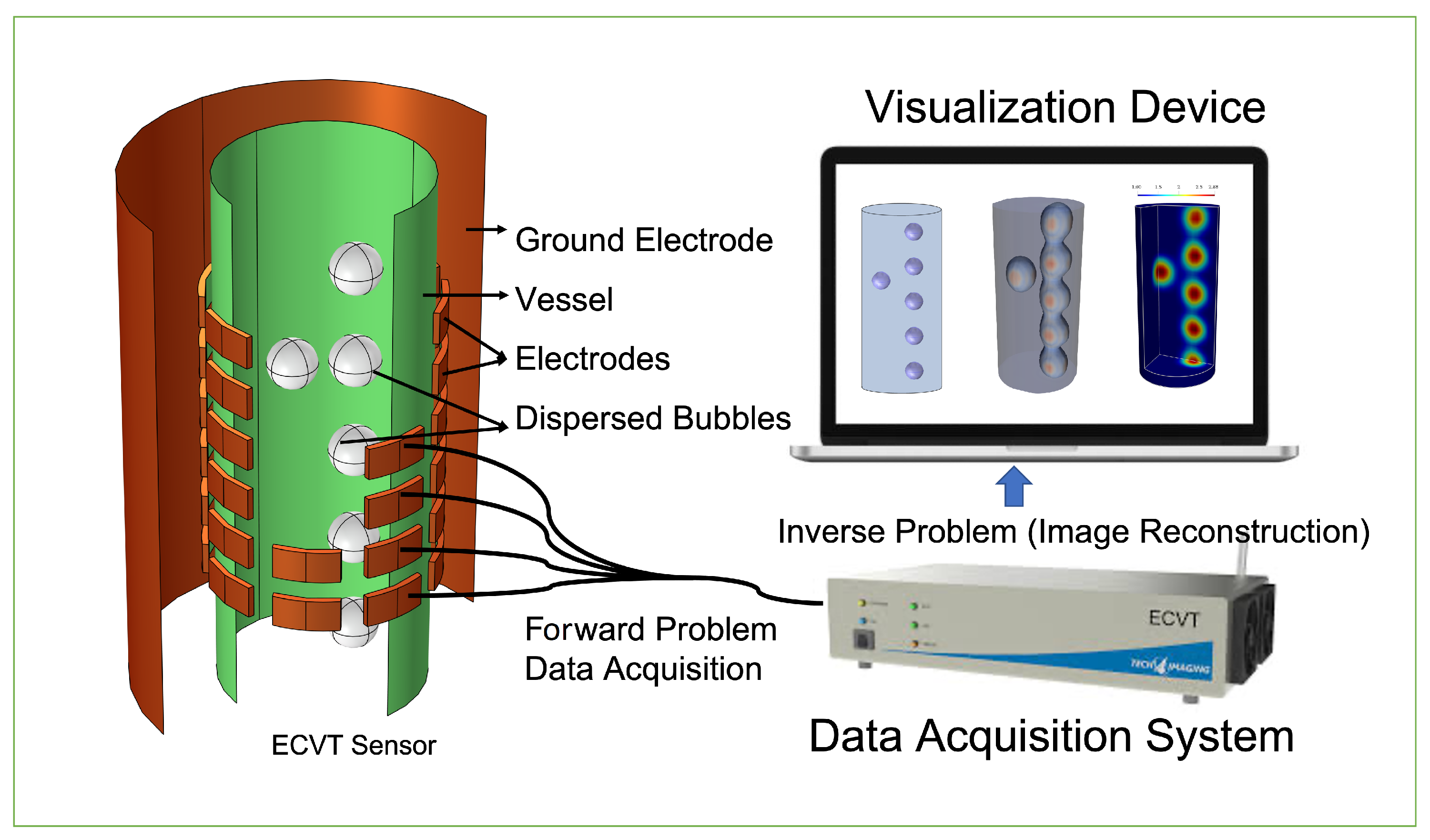
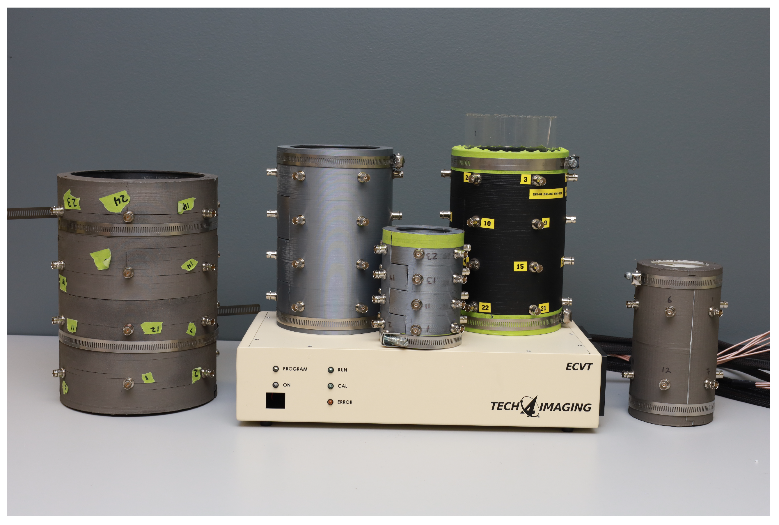
2. Electrical Capacitance Volume Tomography
2.1. Forward Problem
2.2. Inverse Problem
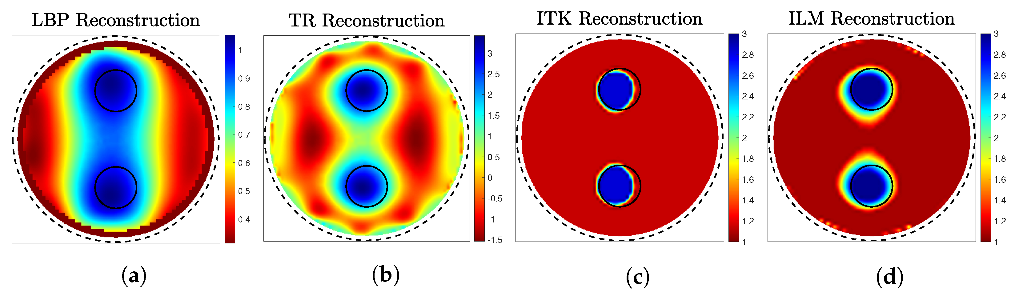
2.2.1. Linear Back-Projection
2.2.2. Pseudo-Inverse with Tikhonov Regularization
2.2.3. Iterative Tikhonov Regularization
2.2.4. Iterative Landweber Method
2.2.5. Non-Traditional Reconstruction Algorithms
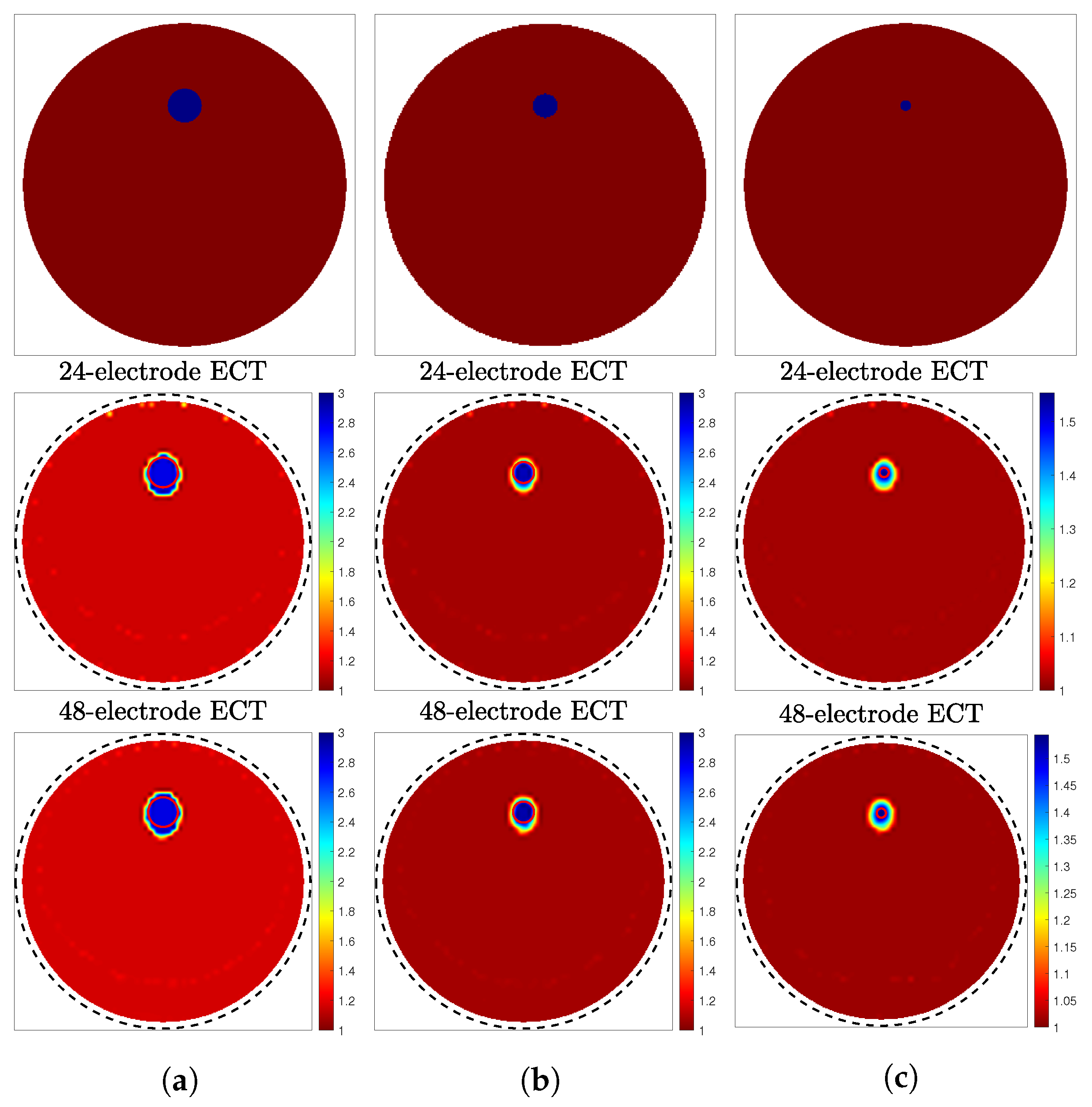
2.3. Sensitivity Matrix Computation
2.4. Selected Open Challenges
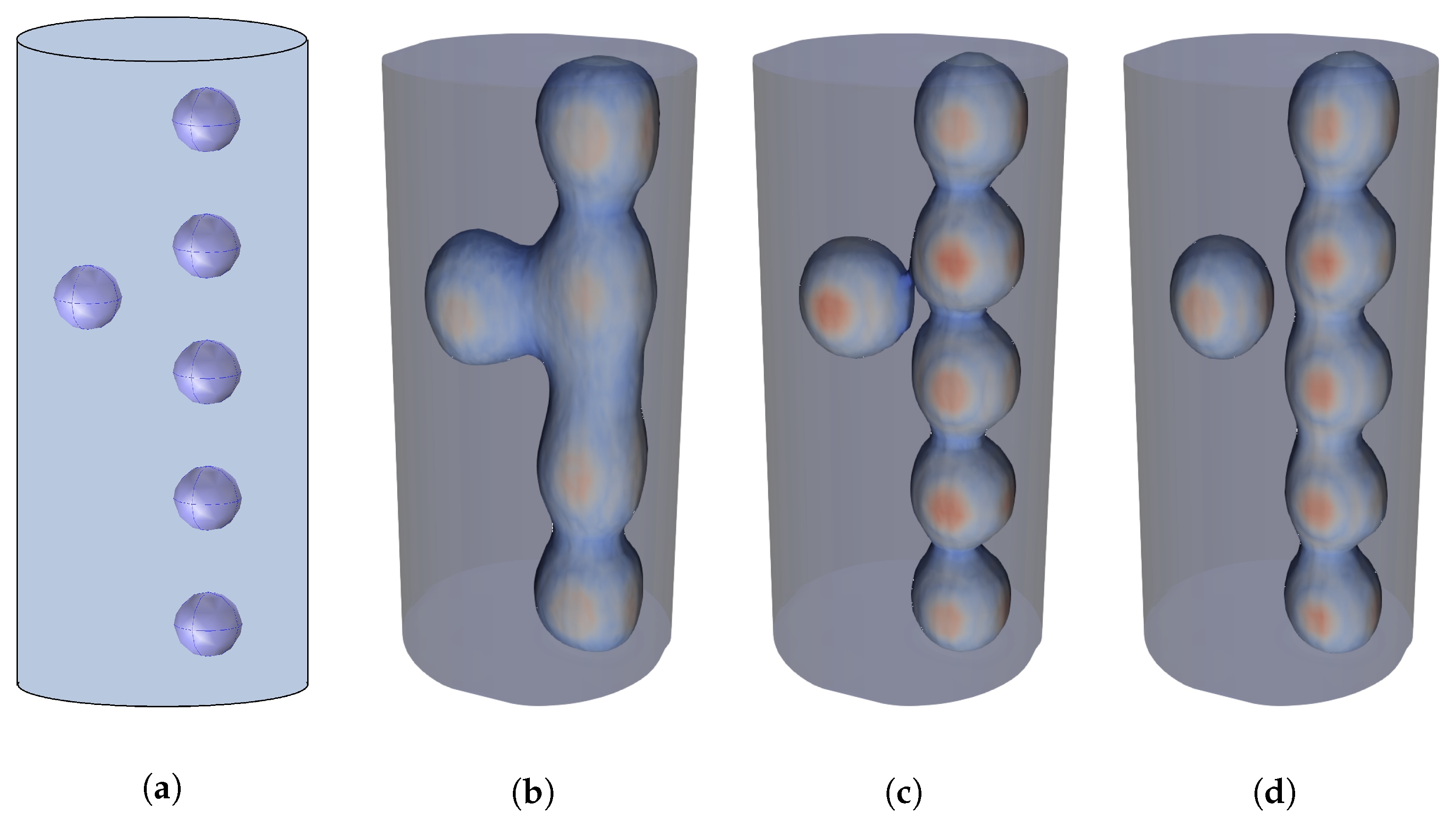
3. Simultaneous Permittivity/Conductivity ECVT-Based Reconstruction
4. Displacement Current Phase Tomography
5. Maxwell–Wagner–Sillars Effect in ECVT Applications
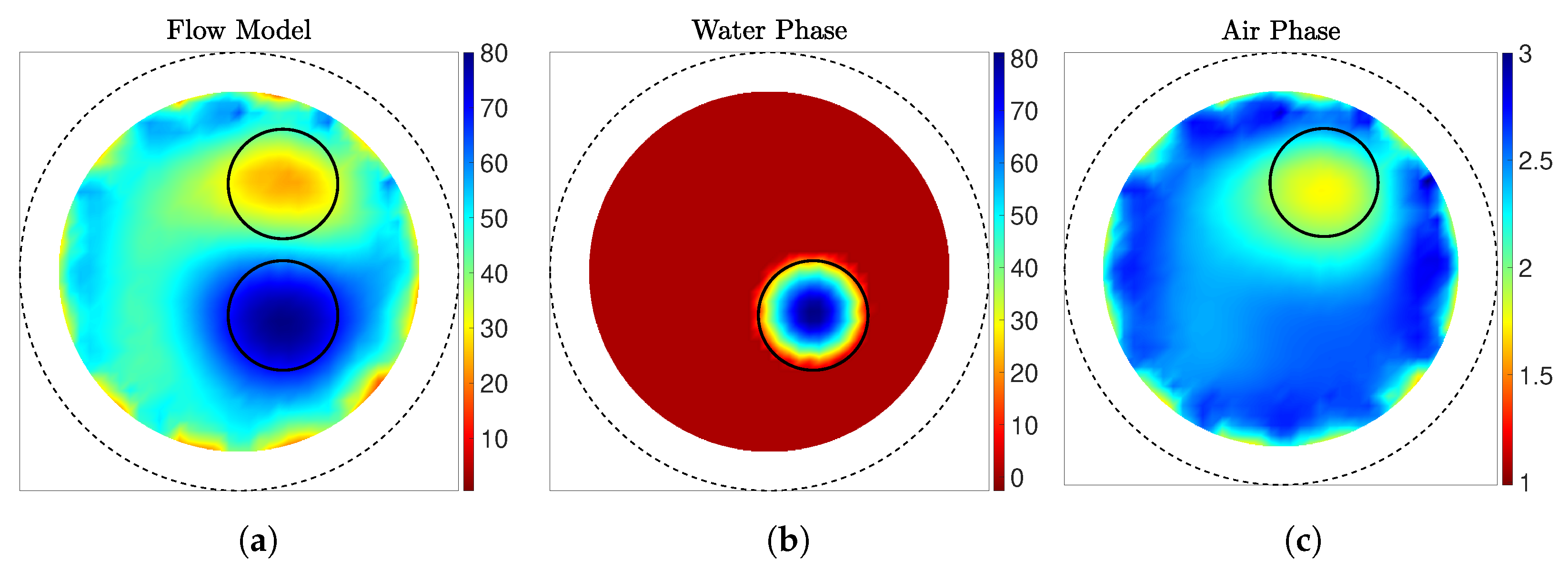
5.1. MWS-ECT Imaging of Water-Containing Flows
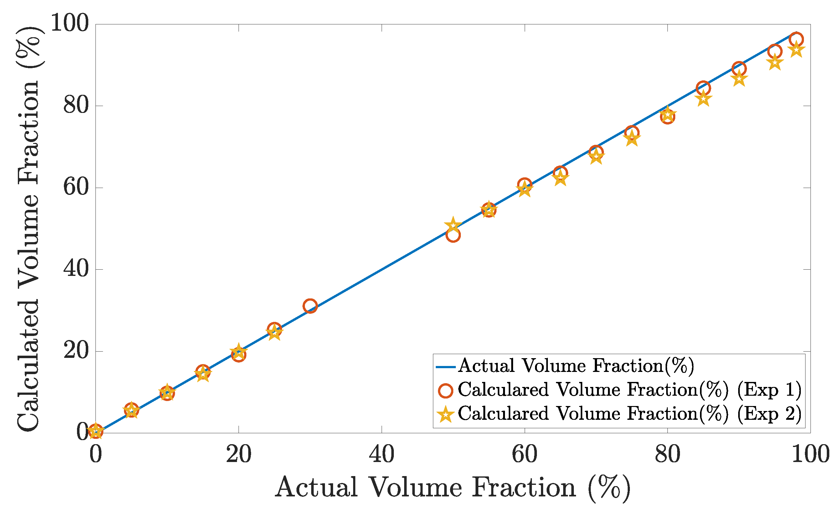
5.2. Volume Fraction Estimation in Homogenized Water-Containing Flows
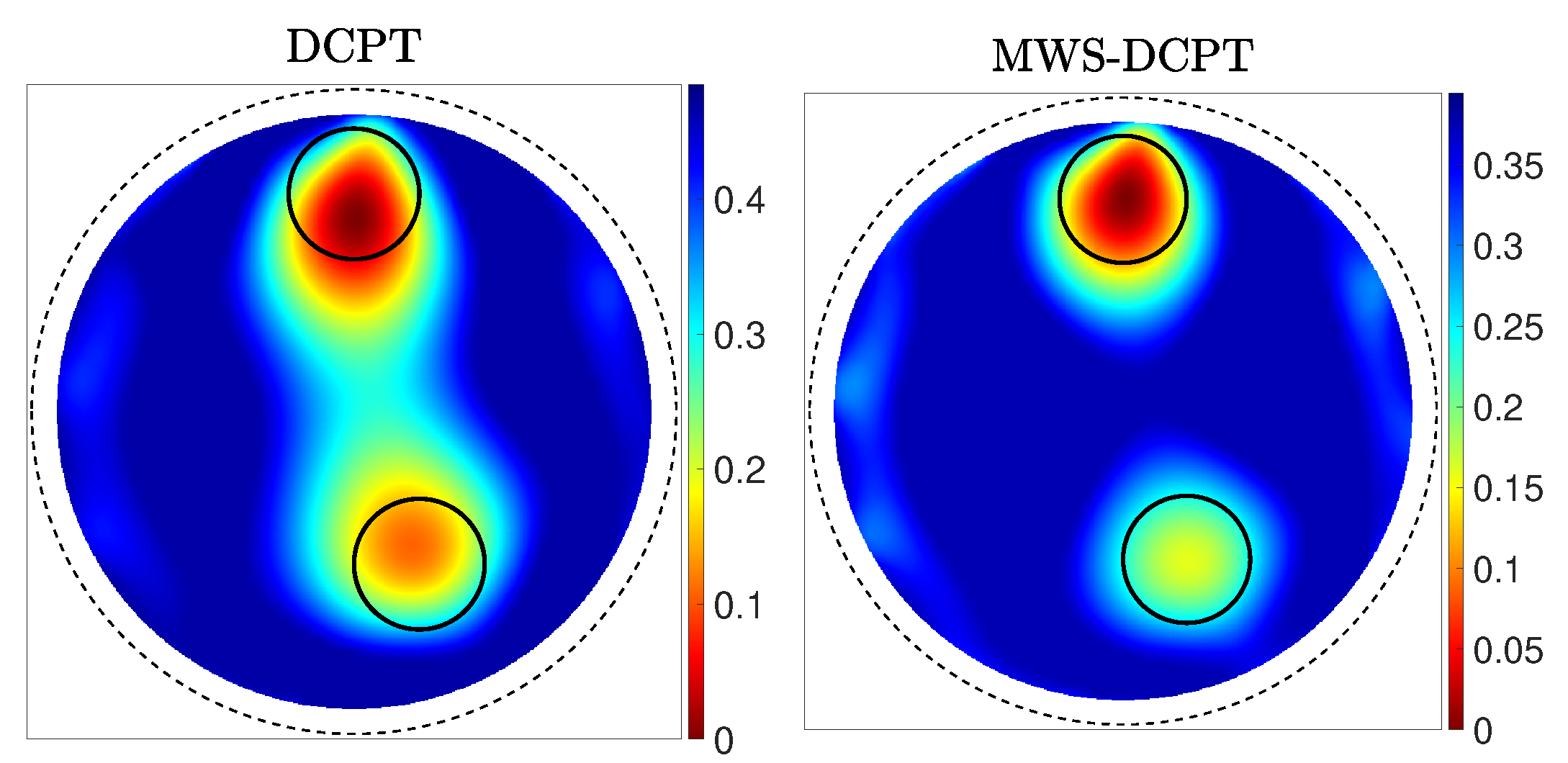
5.3. MWS-DCPT
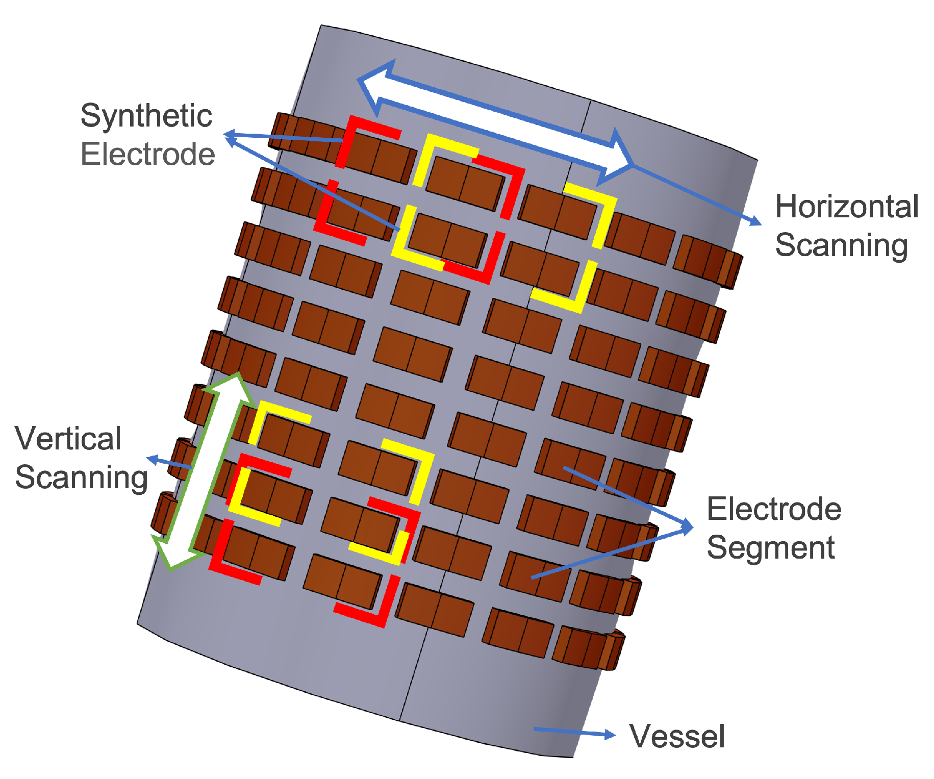
6. Adaptive ECVT
Flexible Sensitivity Matrix for AECVT
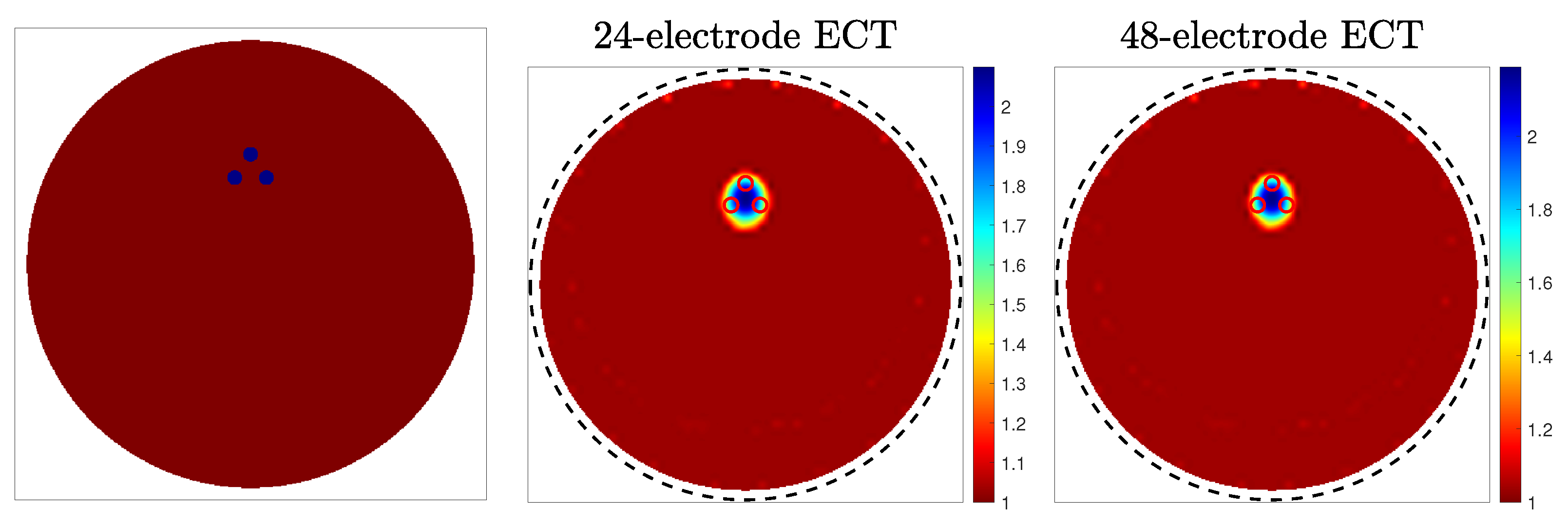
7. Cross-Plane Acquisition Technique for ECVT
8. ECVT-Based Flow Velocimetry
8.1. Cross-Correlation Based Velocity Calculation
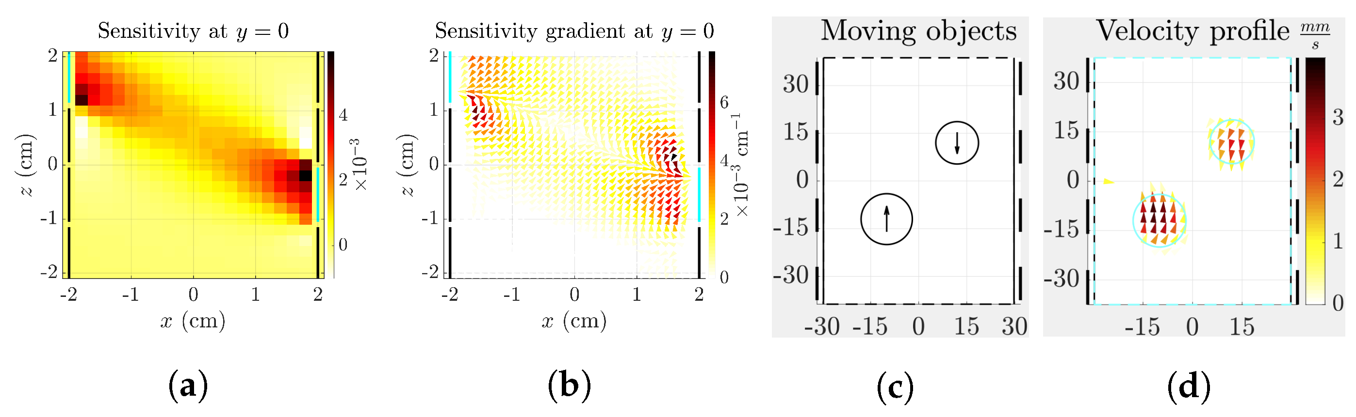
8.2. Sensitivity Gradient-Based Velocity Calculation
9. Machine Learning in ECT/ECVT
9.1. ML-Based Flow Characterization
9.2. ML-Based Image Reconstruction
9.2.1. ECT Image Reconstruction Using Neural Networks
9.2.2. LSSVM-Based Image Reconstruction
9.2.3. RBF-NN Based Image Reconstruction
9.2.4. Auto-Encoder Image Reconstruction
9.2.5. Deep-Learning-Compensated Image Reconstruction Algorithms
9.2.6. Adversarial ML Models for Based Image Reconstruction
9.2.7. Relevance Vector Machine (RVM) and Uncertainty Quantification
10. Conclusions and Look Ahead
Author Contributions
Funding
Institutional Review Board Statement
Informed Consent Statement
Data Availability Statement
Conflicts of Interest
Abbreviations
| ECT | Electrical Capacitance Tomography |
| ECVT | Electrical Capacitance Volume Tomography |
| AECVT | Adaptive Electrical Capacitance Volume Tomography |
| DCPT | Displacement Current Phase Tomography |
| MWS | Maxwell-Wagner-Sillars |
| VoI | Volume of Interest |
| LBP | Linear Back Projection |
| TR | Tikhonov Regularization |
| ITR | Iterative Tikhonov Regularization |
| ILM | Iterative Landweber Method |
| ML | Machine Learning |
| CNN | Convolutional Neural Network |
| DNN | Deep Neural Network |
| LSSVM | Least Square Support Vector Machine |
| RBF | Radial Basis Function |
| RVM | Relevance Vector Machine |
References
- Fan, L.S. Gas-Liquid-Solid Fluidization Engineering; Butterworth-Heinemann: Boston, MA, USA, 1989. [Google Scholar] [CrossRef]
- Han, C.D. Multiphase flow in polymer processing. In Rheology; Springer: Berlin/Heidelberg, Germany, 1980; pp. 121–128. [Google Scholar]
- Khodakov, A.Y.; Chu, W.; Fongarland, P. Advances in the development of novel cobalt Fischer- Tropsch catalysts for synthesis of long-chain hydrocarbons and clean fuels. Chem. Rev. 2007, 107, 1692–1744. [Google Scholar] [CrossRef] [PubMed]
- Awaleh, M.O.; Soubaneh, Y.D. Waste water treatment in chemical industries: The concept and current technologies. Hydrol. Curr. Res. 2014, 5, 1. [Google Scholar]
- Weber, J.M.; Mei, J.S. Bubbling fluidized bed characterization using Electrical Capacitance Volume Tomography (ECVT). Powder Technol. 2013, 242, 40–50. [Google Scholar] [CrossRef]
- Nadeem, H.; Heindel, T.J. Review of noninvasive methods to characterize granular mixing. Powder Technol. 2018, 332, 331–350. [Google Scholar] [CrossRef] [Green Version]
- Perera, K.; Pradeep, C.; Mylvaganam, S.; Time, R.W. Imaging of oil-water flow patterns by Electrical Capacitance Tomography. Flow Meas. Instrum. 2017, 56, 23–34. [Google Scholar] [CrossRef]
- Guo, Q.; Meng, S.; Wang, D.; Zhao, Y.; Ye, M.; Yang, W.; Liu, Z. Investigation of gas–solid bubbling fluidized beds using ECT with a modified Tikhonov regularization technique. AIChE J. 2018, 64, 29–41. [Google Scholar] [CrossRef]
- Warsito, W.; Marashdeh, Q.; Fan, L.S. Electrical Capacitance Volume Tomography. IEEE Sens. J. 2007, 7, 525–535. [Google Scholar] [CrossRef]
- Wang, A.; Marashdeh, Q.M.; Teixeira, F.L.; Fan, L.S. Electrical capacitance volume tomography: A comparison between 12 and and 24-channels sensor systems. Prog. Electromagn. Res. 2015, 41, 73–84. [Google Scholar] [CrossRef] [Green Version]
- Wang, A.; Marashdeh, Q.; Motil, B.J.; Fan, L.S. Electrical capacitance volume tomography for imaging of pulsating flows in a trickle bed. Chem. Eng. Sci. 2014, 119, 77–87. [Google Scholar] [CrossRef]
- Alme, K.J.; Mylvaganam, S. Electrical Capacitance Tomography–Sensor Models, Design, Simulations, and Experimental Verification. IEEE Sens. J. 2006, 6, 1256–1266. [Google Scholar] [CrossRef]
- Li, Y.; Yang, W.; Xie, C.G.; Huang, S.; Wu, Z.; Tsamakis, D.; Lenn, C. Gas/oil/water flow measurement by electrical capacitance tomography. Meas. Sci. Technol. 2013, 24, 074001. [Google Scholar] [CrossRef]
- Liao, A.; Zhou, Q. Application of ECT and relative change ratio of capacitances in probing anomalous objects in water. Flow Meas. Instrum. 2015, 45, 7–17. [Google Scholar] [CrossRef]
- Li, Y.; Holland, D.J. Optimizing the geometry of three-dimensional electrical capacitance tomography sensors. IEEE Sens. J. 2015, 15, 1567–1574. [Google Scholar] [CrossRef]
- Marashdeh, Q.M.; Teixeira, F.L.; Fan, L.S. Electrical capacitance tomography. In Industrial Tomography; Wang, M., Ed.; Woodhead/Elsevier: Cambridge, UK, 2015; pp. 3–21. [Google Scholar]
- Xie, C.; Huang, S.; Beck, M.; Hoyle, B.; Thorn, R.; Lenn, C.; Snowden, D. Electrical capacitance tomography for flow imaging: System model for development of image reconstruction algorithms and design of primary sensors. IEE Proc. G (Circuits Devices Syst.) 1992, 139, 89–98. [Google Scholar] [CrossRef] [Green Version]
- Huang, S.; Xie, C.; Salkeld, J.; Plaskowski, A.; Thorn, R.; Williams, R.; Hunt, A.; Beck, M. Process tomography for identification, design and measurement in industrial systems. Powder Technol. 1992, 69, 85–92. [Google Scholar] [CrossRef]
- Yang, W.; Beck, M.; Byars, M. Electrical capacitance tomography—From design to applications. Meas. Control 1995, 28, 261–266. [Google Scholar] [CrossRef]
- Williams, R.A.; Beck, M.S. Process Tomography; Butterworth-Heinemann: Oxford, UK, 1995. [Google Scholar] [CrossRef]
- Dyakowski, T.; Edwards, R.; Xie, C.; Williams, R.A. Application of capacitance tomography to gas-solid flows. Chem. Eng. Sci. 1997, 52, 2099–2110. [Google Scholar] [CrossRef]
- Yang, W.Q.; Peng, L. Image reconstruction algorithms for electrical capacitance tomography. Meas. Sci. Technol. 2003, 14, R1. [Google Scholar] [CrossRef]
- Watzenig, D.; Fox, C. A review of statistical modelling and inference for electrical capacitance tomography. Meas. Sci. Technol. 2009, 20, 052002. [Google Scholar] [CrossRef]
- Marashdeh, Q.; Teixeira, F.L. Sensitivity matrix calculation for fast 3-D electrical capacitance tomography (ECT) of flow systems. IEEE Trans. Magn. 2004, 40, 1204–1207. [Google Scholar] [CrossRef]
- Kim, Y.S.; Lee, S.H.; Ijaz, U.Z.; Kim, K.Y.; Choi, B.Y. Sensitivity map generation in electrical capacitance tomography using mixed normalization models. Meas. Sci. Technol. 2007, 18, 2092. [Google Scholar] [CrossRef]
- Guo, Z.; Shao, F.; Lv, D. Sensitivity matrix construction for electrical capacitance tomography based on the difference model. Flow Meas. Instrum. 2009, 20, 95–102. [Google Scholar] [CrossRef]
- Lu, G.; Peng, L.; Zhang, B.; Liao, Y. Preconditioned Landweber iteration algorithm for electrical capacitance tomography. Flow Meas. Instrum. 2005, 16, 163–167. [Google Scholar] [CrossRef]
- Li, Y.; Yang, W. Image reconstruction by nonlinear Landweber iteration for complicated distributions. Meas. Sci. Technol. 2008, 19, 094014. [Google Scholar] [CrossRef]
- Jang, J.D.; Lee, S.H.; Kim, K.Y.; Choi, B.Y. Modified iterative Landweber method in electrical capacitance tomography. Meas. Sci. Technol. 2006, 17, 1909. [Google Scholar] [CrossRef]
- Yang, W.Q.; Spink, D.M.; York, T.A.; McCann, H. An image-reconstruction algorithm based on Landweber’s iteration method for electrical-capacitance tomography. Meas. Sci. Technol. 1999, 10, 1065–1069. [Google Scholar] [CrossRef]
- Ye, J.; Wang, H.; Yang, W. Image Reconstruction for Electrical Capacitance Tomography Based on Sparse Representation. IEEE Trans. Instrum. Meas. 2015, 64, 89–102. [Google Scholar] [CrossRef]
- de Moura, H.L.; Pipa, D.R.; Wrasse, A.d.N.; da Silva, M.J. Image Reconstruction for Electrical Capacitance Tomography Through Redundant Sensitivity Matrix. IEEE Sens. J. 2017, 17, 8157–8165. [Google Scholar] [CrossRef]
- Soleimani, M.; Lionheart, W.R. Nonlinear image reconstruction for electrical capacitance tomography using experimental data. Meas. Sci. Technol. 2005, 16, 1987. [Google Scholar] [CrossRef]
- Marashdeh, Q.; Warsito, W.; Fan, L.S.; Teixeira, F.L. A Multimodal Tomography System Based on ECT Sensors. IEEE Sens. J. 2007, 7, 426–433. [Google Scholar] [CrossRef]
- Marashdeh, Q.; Warsito, W.; Fan, L.S.; Teixeira, F.L. Dual imaging modality of granular flow based on ECT sensors. Granul. Matter 2008, 10, 75–80. [Google Scholar] [CrossRef]
- Zhang, M.; Soleimani, M. Simultaneous reconstruction of permittivity and conductivity using multi-frequency admittance measurement in electrical capacitance tomography. Meas. Sci. Technol. 2016, 27, 025405. [Google Scholar] [CrossRef] [Green Version]
- Gunes, C.; Marashdeh, Q.; Teixeira, F. A Comparison Between Electrical Capacitance Tomography and Displacement-Current Phase Tomography. IEEE Sens. J. 2017, 17, 8037–8046. [Google Scholar] [CrossRef]
- Rasel, R.K.; Zuccarelli, C.; Marashdeh, Q.; Fan, L.S.; Teixeira, F.L. Towards Multiphase Flow Decomposition Based on Electrical Capacitance Tomography Sensors. IEEE Sens. J. 2017, 17, 8027–8036. [Google Scholar] [CrossRef]
- Rasel, R.K.; Marashdeh, Q.; Teixeira, F.L. Toward Electrical Capacitance Tomography of Water-Dominated Multiphase Vertical Flows. IEEE Sens. J. 2018, 18, 10041–10048. [Google Scholar] [CrossRef]
- Becher, P. Dielectric Properties of Emulsions and Related Systems, Encyclopedia of Emulsion Technology; M. Dekker: New York, NY, USA, 1983. [Google Scholar]
- Maxwell, J.C. A Treatise on Electricity and Magnetism; Clarendon: Oxford, UK, 1892. [Google Scholar]
- Wagner, K.W. The after effect in dielectrics. Arch. Electrotech. 1914, 2, 378. [Google Scholar]
- Sillars, R. The properties of a dielectric containing semiconducting particles of various shapes. Inst. Electr. Eng. Proc. Wirel. Sect. Inst. 1937, 12, 378–394. [Google Scholar]
- Sihvola, A.H.; Lindell, I.V. Chiral Maxwell-Garnett mixing formula. Electron. Lett. 1990, 26, 118–119. [Google Scholar] [CrossRef]
- Hanai, T. Theory of the dielectric dispersion due to the interfacial polarization and its application to emulsions. Kolloid-Zeitschrift 1960, 171, 23–31. [Google Scholar] [CrossRef]
- Hossain, M.S.; Abir, M.T.; Alam, M.S.; Volakis, J.L.; Islam, M.A. An Algorithm to Image Individual Phase Fractions of Multiphase Flows Using Electrical Capacitance Tomography. IEEE Sens. J. 2020, 20, 14924–14931. [Google Scholar] [CrossRef]
- Rasel, R.K.; Straiton, B.; Marashdeh, Q.; Teixeira, F.L. Toward Water Volume Fraction Calculation in Multiphase Flows Using Electrical Capacitance Tomography Sensors. IEEE Sens. J. 2020, 21, 7702–7712. [Google Scholar] [CrossRef]
- Rasel, R.K.; Straiton, B.J.; Solon, A.; Marashdeh, Q.M.; Teixeira, F.L. Deep Learning Based Volume Fraction Estimation for Two-Phase Water-Containing Flows. In Proceedings of the 2021 IEEE Sensors, Sydney, Australia, 31 October–3 November 2021; pp. 1–4. [Google Scholar] [CrossRef]
- Rasel, R.K.; Gunes, C.; Marashdeh, Q.M.; Teixeira, F.L. Exploiting the Maxwell-Wagner-Sillars Effect for Displacement-Current Phase Tomography of Two-Phase Flows. IEEE Sens. J. 2017, 17, 7317–7324. [Google Scholar] [CrossRef]
- Ospina Acero, D.; Chowdhury, S.M.; Marashdeh, Q.M.; Teixeira, F.L. Efficient and Flexible Sensitivity Matrix Computation for Adaptive Electrical Capacitance Volume Tomography. IEEE Trans. Instrum. Meas. 2021, 70, 1–10. [Google Scholar] [CrossRef]
- Chowdhury, S.M.; Marashdeh, Q.M.; Teixeira, F.L. Electronic Scanning Strategies in Adaptive Electrical Capacitance Volume Tomography: Tradeoffs and Prospects. IEEE Sens. J. 2020, 20, 9253–9264. [Google Scholar] [CrossRef]
- Zeeshan, Z.; Zuccarelli, C.E.; Acero, D.O.; Marashdeh, Q.M.; Teixeira, F.L. Enhancing Resolution of Electrical Capacitive Sensors for Multiphase Flows by Fine-Stepped Electronic Scanning of Synthetic Electrodes. IEEE Trans. Instrum. Meas. 2019, 68, 462–473. [Google Scholar] [CrossRef]
- Marashdeh, Q.M.; Teixeira, F.L.; Fan, L.S. Adaptive electrical capacitance volume tomography. IEEE Sens. J. 2014, 14, 1253–1259. [Google Scholar] [CrossRef]
- Zeeshan, Z.; Teixeira, F.; Marashdeh, Q. Sensitivity map computation in adaptive electrical capacitance volume tomography with multielectrode excitations. Electron. Lett. 2015, 51, 334–336. [Google Scholar] [CrossRef]
- Zhao, J.; Zou, X.; Fu, W. Sensitivity map analysis of adaptive electrical capacitance volume tomography using nonuniform voltage excitation envelopes. IEEE Sens. J. 2017, 17, 105–112. [Google Scholar] [CrossRef]
- Song, P.; Zhao, J.; Fu, W.; Xia, T. Image reconstruction in adaptive electrical capacitance volume tomography using nonuniform voltage excitation envelopes. In Proceedings of the 2017 3rd IEEE International Conference on Computer and Communications (ICCC), Chengdu, China, 13–16 December 2017; pp. 1907–1911. [Google Scholar] [CrossRef]
- Ospina-Acero, D.; Marashdeh, Q.M.; Teixeira, F.L. Relevance Vector Machine Image Reconstruction Algorithm for Electrical Capacitance Tomography With Explicit Uncertainty Estimates. IEEE Sens. J. 2020, 20, 4925–4939. [Google Scholar] [CrossRef]
- Rasel, R.K.; Sines, J.N.; Marashdeh, Q.; Teixeira, F.L. Cross-plane acquisitions in electrical capacitance volume tomography. IEEE Sens. J. 2019, 19, 8767–8774. [Google Scholar] [CrossRef]
- Li, Y.; Holland, D.J. Fast and robust 3D electrical capacitance tomography. Meas. Sci. Technol. 2013, 24, 105406. [Google Scholar] [CrossRef] [Green Version]
- Saoud, A.; Mosorov, V.; Grudzien, K. Measurement of velocity of gas/solid swirl flow using Electrical Capacitance Tomography and cross correlation technique. Flow Meas. Instrum. 2017, 53, 133–140. [Google Scholar] [CrossRef]
- Yang, W. Design of electrical capacitance tomography sensors. Meas. Sci. Technol. 2010, 21, 042001. [Google Scholar] [CrossRef]
- Warsito, W.; Fan, L.S. 3D-ECT velocimetry for flow structure quantification of gas-liquid–solid fluidized beds. Can. J. Chem. Eng. 2003, 81, 875–884. [Google Scholar] [CrossRef]
- Botton, L.F.; de Moura, H.L.; Wrasse, A.N.; Pipa, D.R.; Morales, R.E.; da Silva, M.J. Twin Direct-Imaging Sensor for Flow Velocity Profiling in Two-Phase Mixtures. In Proceedings of the 2018 IEEE Sensors, New Delhi, India, 28–31 October 2018; pp. 1–4. [Google Scholar]
- Chowdhury, S.; Marashdeh, Q.M.; Teixeira, F.L. Velocity Profiling of Multiphase Flows Using Capacitive Sensor Sensitivity Gradient. IEEE Sens. J. 2016, 16, 8365–8373. [Google Scholar] [CrossRef]
- Park, C.; Chowdhury, S.M.; Pottimurthy, Y.; Marashdeh, Q.M.; Tong, A.; Teixeira, F.L.; Fan, L.S. Velocity profiling of a gas-solid fluidized bed using electrical capacitance volume tomography. IEEE Trans. Instrum. Meas. 2022, accepted. [Google Scholar] [CrossRef]
- Chowdhury, S.M.; Park, C.; Pottimurthy, Y.; Marashdeh, Q.M.; Teixeira, F.L.; Fan, L.S. Robust Automated Stopping Criterion for Semi-Convergent Image and Velocity Reconstruction in Electrical Capacitance Volume Tomography. IEEE Open J. Instrum. Meas. in review. 2022. [Google Scholar]
- Gunes, C.; Chowdhury, S.M.; Zuccarelli, C.E.; Marashdeh, Q.M.; Teixeira, F.L. Displacement-current phase tomography for water-dominated two-phase flow velocimetry. IEEE Sens. J. 2018, 19, 1563–1571. [Google Scholar] [CrossRef]
- Zhang, L.; Wang, H. Identification of oil—Gas two-phase flow pattern based on SVM and electrical capacitance tomography technique. Flow Meas. Instrum. 2010, 21, 20–24. [Google Scholar] [CrossRef]
- Marashdeh, Q.; Warsito, W.; Fan, L.S.; Teixeira, F.L. A nonlinear image reconstruction technique for ECT using a combined neural network approach. Meas. Sci. Technol. 2006, 17, 2097. [Google Scholar] [CrossRef]
- Chen, E.; Sarris, C.D. A Multi-Level Reconstruction Algorithm for Electrical Capacitance Tomography Based on Modular Deep Neural Networks. In Proceedings of the 2019 IEEE International Symposium on Antennas and Propagation and USNC-URSI Radio Science Meeting, Atlanta, GA, USA, 7–12 July 2019; pp. 223–224. [Google Scholar] [CrossRef]
- Chen, X.; Hu, H.l.; Liu, F.; Gao, X.X. Image reconstruction for an electrical capacitance tomography system based on a least-squares support vector machine and a self-adaptive particle swarm optimization algorithm. Meas. Sci. Technol. 2011, 22, 104008. [Google Scholar] [CrossRef]
- Wang, H.; Hu, H.l.; Wang, L.j.; Wang, H.x. Image reconstruction for an Electrical Capacitance Tomography (ECT) system based on a least squares support vector machine and bacterial colony chemotaxis algorithm. Flow Meas. Instrum. 2012, 27, 59–66. [Google Scholar] [CrossRef]
- Xia, C.; Hongli, H.; ZHANG, J.; Qulan, Z. An ECT system based on improved RBF network and adaptive wavelet image enhancement for solid/gas two-phase flow. Chin. J. Chem. Eng. 2012, 20, 359–367. [Google Scholar]
- Zheng, J.; Peng, L. An autoencoder-based image reconstruction for electrical capacitance tomography. IEEE Sens. J. 2018, 18, 5464–5474. [Google Scholar] [CrossRef]
- Zheng, J.; Li, J.; Li, Y.; Peng, L. A benchmark dataset and deep learning-based image reconstruction for electrical capacitance tomography. Sensors 2018, 18, 3701. [Google Scholar] [CrossRef] [PubMed] [Green Version]
- Zheng, J.; Ma, H.; Peng, L. A CNN-based image reconstruction for electrical capacitance tomography. In Proceedings of the 2019 IEEE International Conference on Imaging Systems and Techniques (IST), Abu Dhabi, United Arab Emirates, 9–10 December 2019; pp. 1–6. [Google Scholar]
- Zheng, J.; Peng, L. A deep learning compensated back projection for image reconstruction of electrical capacitance tomography. IEEE Sens. J. 2020, 20, 4879–4890. [Google Scholar] [CrossRef]
- Deabes, W.; Abdel-Hakim, A.E.; Bouazza, K.E.; Althobaiti, H. Adversarial Resolution Enhancement for Electrical Capacitance Tomography Image Reconstruction. Sensors 2022, 22, 3142. [Google Scholar] [CrossRef]
- Acero, D.O.; Marashdeh, Q.M.; Teixeira, F.L. Reduced-Space Relevance Vector Machine for Adaptive Electrical Capacitance Volume Tomography. IEEE Trans. Comput. Imaging 2022, 8, 41–53. [Google Scholar] [CrossRef]


| Sensing Modality | Reference(s) | Hardware | Objective(s) | Industrial Application(s) | Comments |
|---|---|---|---|---|---|
| ECT | [18,19,20] | ECT | Imaging | Non-conducting multiphase flow imaging and monitoring | Provides cross-sectional image. |
| ECVT | [9] | ECVT | Imaging, velocimetry, volume fraction estimation | Non-conductive multiphase flow imaging and monitoring | Provides volumetric image. |
| MWS-ECT | [38,39,47,48] | ECT ECVT | Imaging, volume fraction estimation | Water-Containing flow reconstruction and volume estimation | Allows monitoring of water-containing flows using multifrequency and low-frequency excitations. |
| DCPT | [37] | ECT ECVT | Imaging | Water-Continuous flow reconstruction and monitoring | Robust for monitoring water-continuous flows compared to traditional ECT. |
| MWS-DCPT | [49] | ECT ECVT | Imaging | Water-Continuous flow reconstruction and monitoring | Improves imaging resolution of DCPT using multifrequency excitation. |
| Simultaneous , monitoring | [34,35,36] | ECT | Imaging | Water-containing flow reconstruction and monitoring | Complex imaging modality compared to MWS-ECT and DCPT. |
| Cross-plane acquisition optimization | [58,59] | ECVT | Imaging, velocimetry, volume fraction estimation | Multiphase flow monitoring | Reduces computational complexity and improve image quality. |
| AECVT | [50,51,52,53,54,55,56] | ECVT | Imaging, velocimetry, volume fraction estimation | Multiphase flow monitoring | Increases the number of independent measurements without necessarily reducing the effective electrode size. |
| Velocimetry | [60,61,64,67] | ECVT | Velocity profiling | Multiphase flow transport velocity estimation | Commonly used methods are cross-correlation velocimetry and gradient-based velocimetry. |
Publisher’s Note: MDPI stays neutral with regard to jurisdictional claims in published maps and institutional affiliations. |
© 2022 by the authors. Licensee MDPI, Basel, Switzerland. This article is an open access article distributed under the terms and conditions of the Creative Commons Attribution (CC BY) license (https://creativecommons.org/licenses/by/4.0/).
Share and Cite
Rasel, R.K.; Chowdhury, S.M.; Marashdeh, Q.M.; Teixeira, F.L. Review of Selected Advances in Electrical Capacitance Volume Tomography for Multiphase Flow Monitoring. Energies 2022, 15, 5285. https://doi.org/10.3390/en15145285
Rasel RK, Chowdhury SM, Marashdeh QM, Teixeira FL. Review of Selected Advances in Electrical Capacitance Volume Tomography for Multiphase Flow Monitoring. Energies. 2022; 15(14):5285. https://doi.org/10.3390/en15145285
Chicago/Turabian StyleRasel, Rafiul K., Shah M. Chowdhury, Qussai M. Marashdeh, and Fernando L. Teixeira. 2022. "Review of Selected Advances in Electrical Capacitance Volume Tomography for Multiphase Flow Monitoring" Energies 15, no. 14: 5285. https://doi.org/10.3390/en15145285