Article

Optimization of Magnetic Gear Patterns Based on Taguchi Method Combined with Genetic Algorithm

1
College of Information Engineering, Zhejiang University of Technology, Hangzhou 310023, China
2
Department of Electrical Engineering, The Hong Kong Polytechnic University, Hong Kong, China
*
Author to whom correspondence should be addressed.
Energies 2022, 15(14), 4963; https://doi.org/10.3390/en15144963
Submission received: 23 May 2022 / Revised: 12 June 2022 / Accepted: 21 June 2022 / Published: 6 July 2022
(This article belongs to the Special Issue Future Smart Grids with High Integrations of New Technologies)

Abstract

:
Magnetic gears (MGs) have gained increasing attention due to their sound performance in high torque density and low friction loss. Aiming to maximize the torque density, topology design has been a popular issue in recent years. However, studies on the optimization comparisons of a general MG topology pattern are very limited. This paper proposes a Taguchi-method-based optimization method for a general MG topology pattern, which can cover most of the common types of radially magnetized concentric-surface-mounted MGs (RMCSM-MGs). The Taguchi method is introduced to evaluate the influence of each parameter in MGs. Moreover, the parameter value range is re-examined based on the sensitivity analysis results. The genetic algorithm (GA) method is adopted to optimize the topology pattern in the study.

1. Introduction

Wind power generation has become more and more popular in industrial production and daily life due to its clean and inexhaustible advantages over traditional coal-fired power [1]. Gearboxes are widely used in wind power generation systems. Components of different speeds can be made to run at certain speed ratios by connecting them through gearboxes. Mechanical gears, which are currently widely used in industry, suffer from the following problems: loud noise, high manufacturing and installation accuracy requirements, high friction loss, etc., [2]. In recent years, due to the development of rare earth materials, magnetic gears (MGs) are expected to replace mechanical gears [3]. Abundant research and experiments have indicated that the transmission torque of MGs can reach up to 100 kNm/m3 [4]. In addition, MGs have the advantages of physical isolation, lower maintenance costs, and inherent overload protection [5].
The main material required for MGs is rare-earth permanent magnets (PMs), which are expensive. Hence, there is an increasing concern regarding saving PM material without sacrificing the torque density. There have been several longitudinal studies involving optimizing the MG topology to save resources and costs. To meet application requirements, studies on the topology design of radially magnetized concentric-surface-mounted MGs (RMCSM-MGs) have become popular in recent years. It is well-known that RMCSM-MGs are commonly made of three layers. Traditional RMCSM-MGs have PMs embedded in the inner layer and outer layer, while the middle layer is made of ferrite material. Another kind of MG with competitive performance is the triple-PM-excited MGs, which have PMs embedded in each layer. The torque per unit PM volume among the six basic topologies of triple-PM-excited MGs is compared in [6]. However, the six types of topologies have the same outer rotor structure and modulation ring structure. Only the topology of the inner rotor is changed during the comparison. In [7], the author attempted to propose a pattern design for the triple-PM-excited MGs. However, the unipolar permanent magnetic–ferrite array and the air–ferrite array of the inner rotor and modulation ring are not considered in this pattern. Moreover, optimization of the PM and ferrite distribution is mostly ignored in the literature; the assumption that PM and ferrite are equally distributed is taken by default, without any explanation.
Research on this subject has been mostly restricted to individually optimizing each type of MG, which may cost an amount of time. This paper aims to optimize and comprehensively compare the topology of common RMCSM-MGs. Therefore, a topology pattern was designed, which could cover most of the common types of RMCSM-MGs. In previous studies, authors often needed to optimize once for each MG structure [8,9,10]. By resorting to pattern design, optimization must be performed only once [11,12]. The optimization method used in this article is the genetic algorithm (GA). Local convergence, the so-called “premature phenomenon”, is a problem that has always plagued researchers. Common solutions include increasing the probability of mutation, increasing diversity, and reducing the probability of selecting excellent chromosomes [13]. However, these approaches may result in a higher amount of computation. In this paper, the Taguchi method is employed to obtain a near-optimal value, which can help to determine the appropriate initial values and ranges in GA optimization [14,15,16]. The Taguchi method has been widely used in the field of industrial engineering. To name a few applications, the parameters of the Jiles–Atherton hysteresis model are optimized using Taguchi’s method in [17], and the author of [18] blended the Taguchi orthogonal array (OA) concept into the design of the linear antenna array. In [19], the Taguchi method is employed to optimize the material of multiple layers of dielectric thin films in the photonic radiative cooler. Many other applications of the Taguchi method were reviewed in [20,21,22], among other studies.

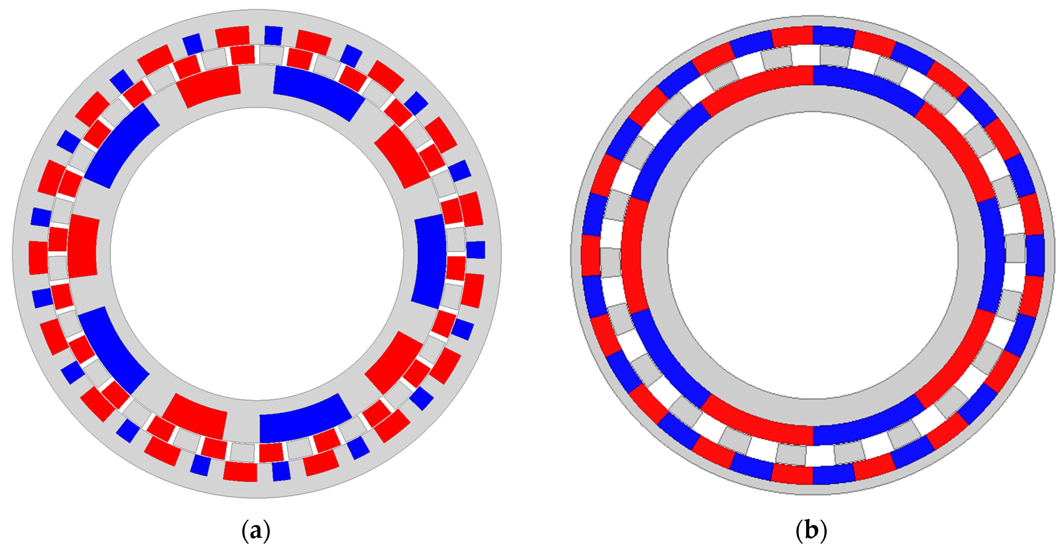
2. General Pattern Design

The RMCSM-MG is mainly composed of three rings. The inner and the outer ring can rotate, so they are named rotors. The middle ring is stationary, and is named the modulation ring. It is worth noting that the PMs of the RMCSM-MG are magnetized in radial directions. As shown in Figure 1, the rotors may be designed as a bipolar PM array, unipolar PM array, or bipolar PM–ferrite array [23]. As presented in Figure 2, the modulation ring may be created as a ferrite–air array, ferrite–PM array, or ferrite–PM–air array [23]. Hence, there are 27 possible topologies of RMGSM-MG, which are discussed in this study. The intuitive approach is to separately optimize each of the 27 types, but this requires a lot of computation. In this article, we design a pattern to cover these 27 special structural types. This can greatly reduce the amount of computation.
The configuration of the RMCSM-MG pattern is shown in Figure 3. It is well-known that the working principle of MGs obeys the modulation effect [24], and the proposed RMGSM-MG pattern in this article is no exception. Figure 4 is a partially enlarged drawing of the RMGSM-MG pattern in Figure 3. The red and blue segments represent the S and N pole PMs made from NdFeB material, respectively. The magnetization directions are marked in the figure. The grey segments are ferrite pieces made of M19_24G material. The flux path of both inner and outer rotor PM poles before modulation is shown. After modulation, the inner rotor flux path has the same pole pair number as that of the outer rotor. Similarly, the outer rotor can be modulated to match the PM pole pair of the inner rotor. Thus, they can transmit torque steadily between each rotor at any different rotational speed. For this reason, the pole pair number of each layer can be summarized by the following equations:
p o = | p i m | o r p i = | p o m |
where pi and po represent the inner and outer pole pair numbers, respectively. The quantity m represents the segment of modulation ferrite.
The parameters of the RMCSM-MG pattern are shown in Table 1. As shown in Figure 3, the innermost radius, Rs = 60 mm, and the outermost radius, Rm = 105 mm, are also constant to keep the total volume of the MG invariable. For each layer, the distribution of PM and ferrite segments is re-examined by setting the expansion angles as variables. It can be deduced that the PM and ferrite arrays shown in Figure 1 and Figure 2 are particular cases included in the general pattern. For instance, Figure 1a shows the rotor arrays when αi1 = αi2 or αo1 = αo2. Figure 1b shows the case when αi1 = 180°/pi, αi2 = 0 or αo1 = 180°/po, αo2 = 0.

3. Sensitivity Analysis and Optimization

By employing a Taguchi-method-based sensitivity analysis, it is possible to discover a near-optimal solution. In this study, the value range in the optimization is refined according to the near-optimal solution. It is well-known that each parameter will be given an upper boundary and lower boundary in a random search optimization algorithm [25,26,27]. In the Taguchi method, each parameter is evaluated on several specific levels [18].
Parameters to be optimized are listed in Table 1. Assume X represents the array of parameters, and C(X) represents the torque per unit PM volume, which can be expressed as follows:
C ( X ) = T ( X ) / V P M ( X )
where T(X) is the average electromagnetic torque of the inner rotor and outer rotor in one rotation period, and VPM(X) is the total volume of the PM pieces. The optimization criterion of this study is to maximize C(X). It is worth noting that the unit of C(X) is kNm/m3.
Some linear constraints are also added to ensure that the geometry is logical:
{ α i 1 + α i 2 360 ° p i α m 1 + α m 2 360 ° n s α o 1 + α 02 360 ° p o h f + h m i + h m o + h r < R m R s 2 · a p
Furthermore, another constraint is added to ensure a high stability of the MG, which is presented as:
T r ( X ) 4 ( Nm )
where Tr(X) is the average torque ripple of the inner rotor and outer rotor. This value is designed as 2% of the common torque density of RMCSM-MG [24]. In this study, the torque and torque ripple values were measured using the finite element method (FEM) [27]. The 2D FEM solver adopted in this study is Ansys Maxwell 16.0.
This section is divided into subheadings as follows.

3.1. Taguchi Orthogonal Array Analysis of Objective Function

In the Taguchi sensitivity analysis, each parameter is designed with three levels as shown in Table 2 [23]. The L27 Taguchi Orthogonal Array (TOA) is applied in the analysis. A total of 27 experiments are involved in L27 TOA, and each experiment examines the parameters in a specific combination of levels. Level combinations, experimental results, and the resultant cost values are listed in Table 3. It is worth noting that L1, L2, and L3 are the abbreviations of level 1, level 2, and level 3, respectively.
Then we need to evaluate the average effect of the parameters. This index is the average of the experimental results for one parameter at a certain level. For example, the average effect of X1 at L1 is calculated using the following equation:
m X 1 , L 1 = 1 9 n = 1 9 C ( n )
where C(n) represents the results of the nth experiment. Using the same method, we obtained the results shown in Table 4.
Suppose the array element [X1, L1] represents the value in column X1 and row L1. The value represents how much the value of L1 of parameter X1 may influence the cost value. The larger the value, the greater the effect. Therefore, we can extract the most influential level for each parameter. The results illustrate that the parameter combination [L1, L1, L1, L3, L3, L2, L3, L3, L1, L2] is the near-optimal solution. Then, an improved value range is obtained around the near-optimal solution, as shown in Table 5. Considering the actual situation in manufacturing, the lower boundaries of hmi, hf and hmo are set to 4 mm.

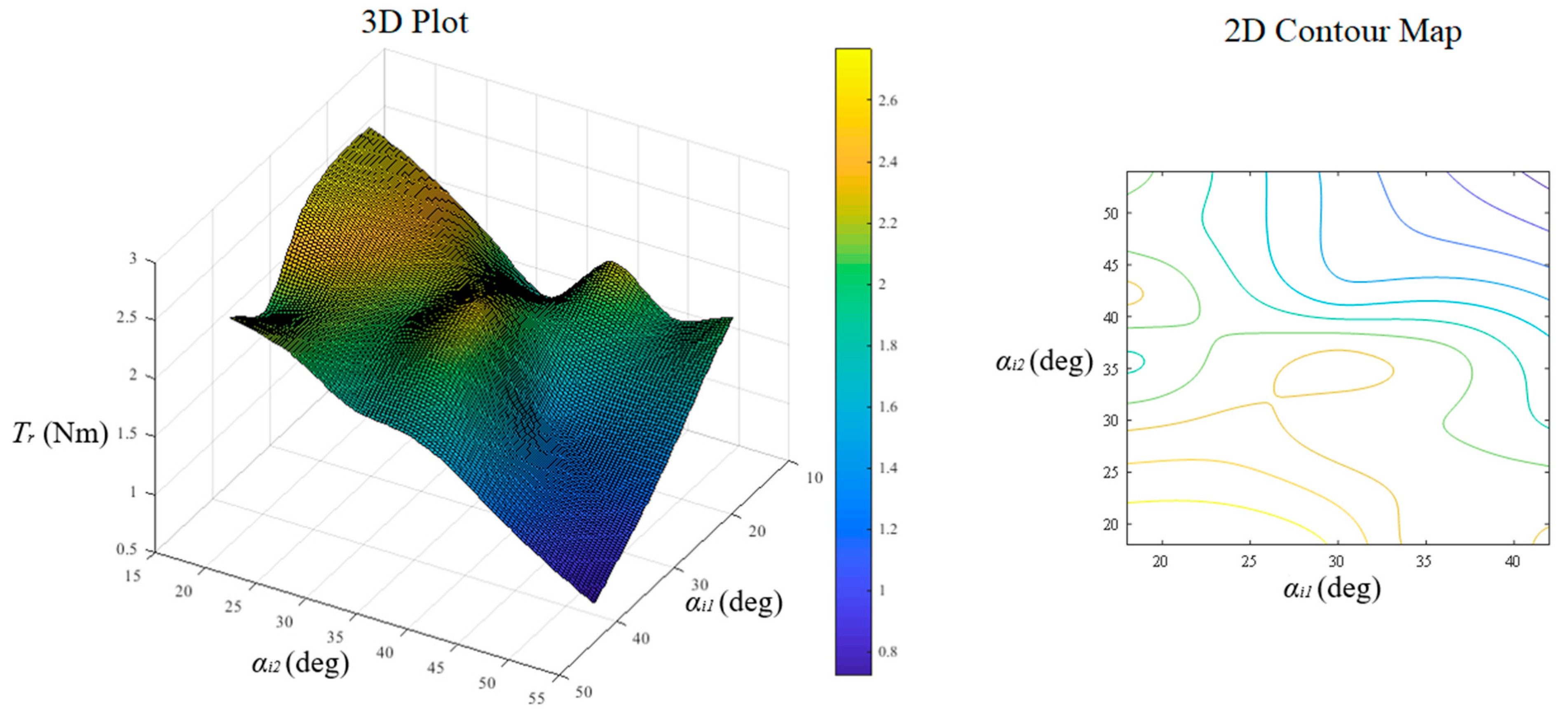
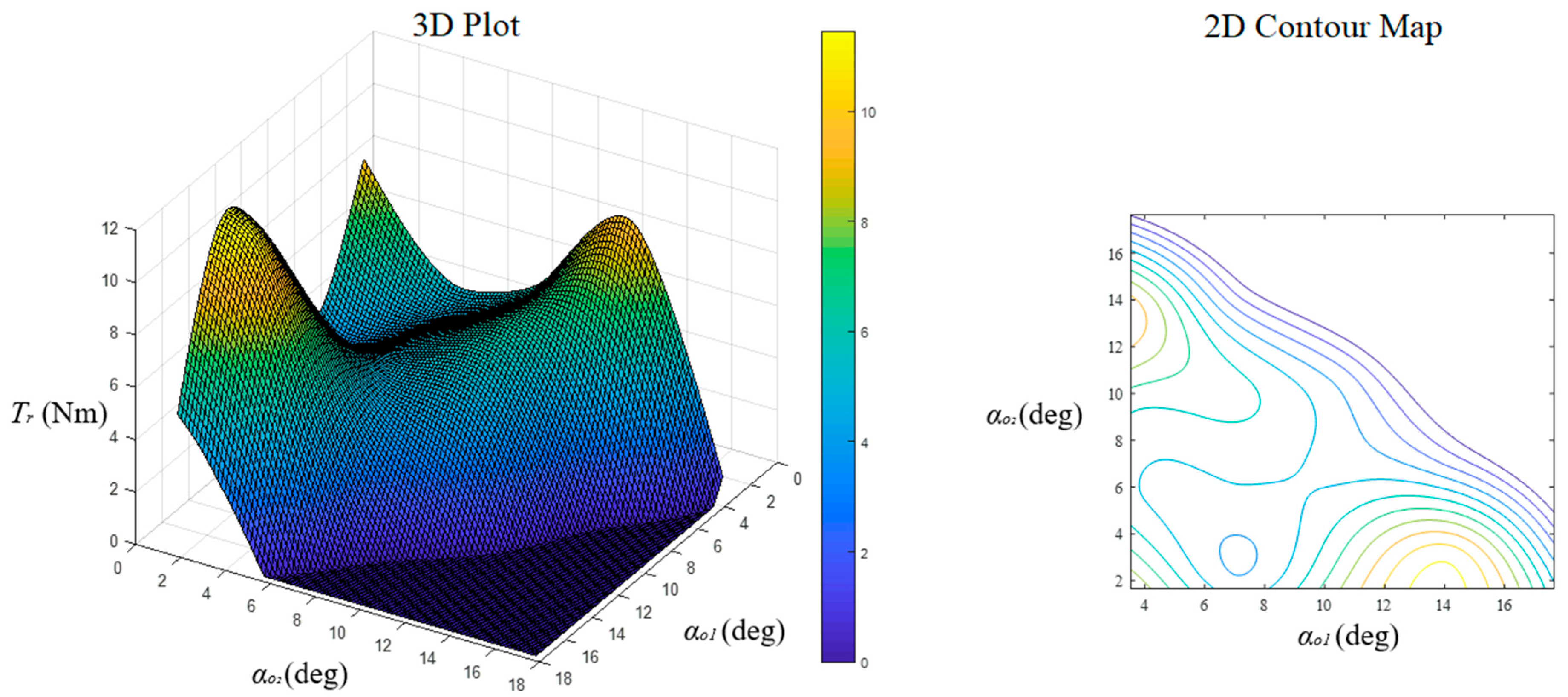
3.2. Sensitivity Analysis and Linear Interpolation Fitting of Torque Ripple Function

To deal with the requirements of the constraint function (4), initially, a study of the sensitivity of each parameter to the constraint function Tr(X) was conducted. Moreover, the most influential parameters were selected to perform the linear interpolation fitting of Tr(X) [28]. Therefore, the value that fulfills the fitting can be considered to be approximately satisfied with the constraint function.
In this study, the parameters are further divided into three levels within the improved value ranges in Table 5. The new level design is shown in Table 6. Then, the L27 TOA, using the parameter level design shown in Table 7, was conducted to obtain the results for Tr(X). Subsequently, the analysis of variance (ANOVA) technique was employed to obtain the influence of each parameter [14]. For instance, the sum of the square of the parameter X1 SSX1 is governed by the formula:
S S X 1 = ( t m X 1 , L 1 t m ) 2 + ( t m X 1 , L 2 t m ) 2 + ( t m X 1 , L 3 t m ) 2
where tm represents the total average Tr(X) value of all experiments. The values tmX1,L1, tmX1,L2, and tmX1,L3 represent the average Tr(X) values of parameter X1 in level 1, level 2, and level 3, respectively. The ANOVA results are shown in Table 7. The SS value represents the degree of sensitivity. The larger the value, the more obvious the influence of this parameter on torque ripple. Table 7 also includes the percentage of influence of each parameter. It can be seen that the parameters X5, X6, X7, and X8 are the four most effective factors on Tr(X). In order to reduce the level of computation, all parameters except for X5, X6, X7, and X8 were ignored in the linear interpolation fitting.
The αi1 and αi2 for the inner layer and the αo1 and αo2 for the outer layer were discussed during fitting. In the sampling process, 20 groups of experimental results of the average torque ripple versus (αi1, αi2) and (αo1, αo2) were obtained. All the parameter values are randomly generated from the improved value range. After the linear interpolation fitting, the curve of the average torque ripple versus (αi1, αi2) and (αo1, αo2) can be achieved, the results of which are shown in Figure 5 and Figure 6. The results in Figure 5 show that the torque ripple fulfils the constraint in all (αi1, αi2) evaluations. It is worth noting that, by introducing the interpolation fitting, the torque ripple may become negative, which is unnatural. Therefore, these values are modified to zero in this study. From the data in Figure 6, a polynomial fitting can be achieved to satisfy the constraint function in (4). The polynomial fitting result is as follows:
α o 2 + 0.001 α o 1 3 0.056 α o 1 2 + 1.625 α o 1 21.73 > 0

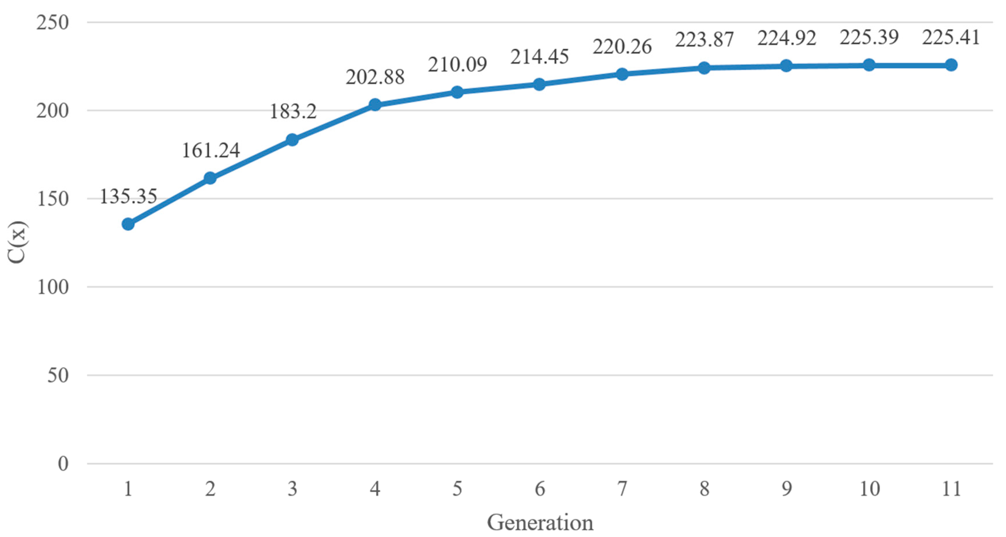
3.3. Establishing Optimization

The last step was to establish optimization by combining the sensitivity analysis results. In this study, we used the GA optimization method refined by the improved value ranges and constraint functions.
The crossover probability was set as 0.7 and the mutation probability was set as 0.15 [29]. The maximum optimization generation Gmax was set as 40, where each generation contained 60 individuals. The convergence condition is as follows:
| C i ( x ) C i 1 ( x ) | 0.1 i = 1 , 2 , , G max
where Ci(x) represents the best solution of the objective function in the ith generation. The optimization is supposed to finish when it attains the convergence condition or reaches the maximum generation.

3.4. Optimization Results Discussions

Without a sensitivity analysis, optimization is performed within a given original value range which may be very costly in terms of time and computational resources. Indeed, the optimization results always fall into local optimality when using the original value range. Therefore, the study of a sensitivity analysis based on the Taguchi method, and the linear interpolation fitting of the torque ripple constraint, is essential. According to the analysis results, the GA optimization is refined with a more precise value range (Table 5) and constraint function (7).
Figure 7 shows the cost value variation in each generation of the refined optimization process. The optimization converges after 11 generations. The configuration and torque performance of both the optimized model and original model are shown in Figure 8 and Figure 9, respectively. The average torque of the inner rotor and outer rotor increases by about 47% after optimization. However, the torque ripple increases by about 17% after optimization but still satisfies the constraint in (4). The average torque per unit PM volume before and after optimization is about 163.72 kNm/m3 and 225.41 kNm/m3, respectively. The average torque per unit PM volume increases by about 38%.
Detailed optimized parameter values are shown in Table 8.

4. Conclusions

The present study makes several noteworthy contributions towards optimizing a general topology pattern for RMCSM-MG. This pattern can cover most of the common types of MGs. The objective is to discover the MG topology with the highest torque per PM volume. Moreover, the torque ripple should be kept within a reasonable range. To discover the optimal topology, the GA optimization method was conducted. In order to reduce the possibility of local convergence and increase the computational cost, the parameter value range was refined using a sensitivity analysis based on the Taguchi method and interpolation fitting. The optimization converges after 11 generations. After optimization, the average torque increases by about 47%, and the average torque per PM volume increases by about 38%.

Author Contributions

Conceptualization, Y.M. and Y.Y.; methodology, Y.M.; software, Y.M.; validation, Y.M. and Y.Y.; formal analysis, Y.M.; investigation, Y.M.; resources, Y.Y.; data curation, Y.M.; writing—original draft preparation, Y.M.; writing—review and editing, Y.Y.; funding acquisition, Y.Y. All authors have read and agreed to the published version of the manuscript.

Funding

This research was funded by Guangdong Basic and Applied Basic Research Foundation 2022A1515010708 and Start-up Fund of PolyU P0036194.

Institutional Review Board Statement

Not applicable.

Informed Consent Statement

Not applicable.

Data Availability Statement

Not applicable.

Conflicts of Interest

The authors declare no conflict of interest.

References

  1. Polinder, H.; Ferreira, J.A.; Jensen, B.B.; Abrahamsen, A.B.; Atallah, K.; McMahon, R.A. Trends in wind turbine generator systems. IEEE Trans. Emerg. Sel. Top. Power Electron. 2013, 1, 174–185. [Google Scholar] [CrossRef]
  2. Rasmussen, P.O.; Andersen, T.O.; Jorgensen, F.T.; Nielsen, O. Development of a high-performance magnetic gear. IEEE Trans. Ind. Appl. 2005, 41, 764–770. [Google Scholar] [CrossRef]
  3. Peng, S.; Fu, W.N.; Ho, S.L. A novel high torque-density triple permanent-magnet-excited magnetic gear. IEEE Trans. Magn. 2014, 50, 6971416. [Google Scholar] [CrossRef]
  4. Atallah, K.; Calverley, S.D.; Howe, D. Design analysis and realisation of a high-performance magnetic gear. IEEE Proc. Elect. Power Appl. 2004, 151, 135–143. [Google Scholar] [CrossRef]
  5. Gouda, E.; Mezani, S.; Baghli, L.; Rezzoug, A. Comparative study between mechanical and magnetic planetary gears. IEEE Trans. Magn. 2011, 47, 439–450. [Google Scholar] [CrossRef]
  6. Niu, S.; Mao, Y. A Comparative Study of Novel Topologies of Magnetic Gears. Energies 2016, 9, 773. [Google Scholar] [CrossRef] [Green Version]
  7. Chen, Y.; Fu, W.N.; Ho, S.L.; Liu, H. A quantitative comparison analysis of radial-flux transverse-flux and axial-flux magnetic gears. IEEE Trans. Magn. 2014, 50, 8104604. [Google Scholar] [CrossRef]
  8. Ho, S.L.; Yang, S.Y.; Ni, G.Z.; Wong, H.C. A particle swarm optimization method with enhanced global search ability for design optimizations of electromagnetic devices. IEEE Trans. Magn. 2006, 42, 1107–1110. [Google Scholar] [CrossRef] [Green Version]
  9. Zhao, X.; Niu, S. Design and Optimization of a New Magnetic-Geared Pole-Changing Hybrid Excitation Machine. IEEE Trans. Ind. Electron. 2017, 64, 9943–9952. [Google Scholar] [CrossRef]
  10. Ho, S.L.; Niu, S.; Fu, W.N. A new dual-stator bidirectional-modulated PM machine and its optimization. IEEE Trans. Magn. 2014, 50, 8103404. [Google Scholar] [CrossRef]
  11. Niu, S.; Chen, N.; Ho, S.L.; Fu, W.N. Design optimization of magnetic gears using mesh adjustable finite-element algorithm for improved torque. IEEE Trans. Magn. 2012, 48, 4156–4159. [Google Scholar] [CrossRef]
  12. Preis, K.; Magele, C.; Biro, O. FEM and evolution strategies in the optimal-design of electromagnetic devices. IEEE Trans. Magn. 1990, 26, 2181–2183. [Google Scholar] [CrossRef]
  13. Dang, D.C.; Friedrich, T.; Kötzing, T.; Krejca, M.S.; Lehre, P.K.; Oliveto, P.S.; Sudholt, D.; Sutton, A.M. Escaping Local Optima Using Crossover With Emergent Diversity. IEEE Trans. Evol. Comput. 2018, 22, 484–497. [Google Scholar] [CrossRef] [Green Version]
  14. Hasanien, H.M. Design optimization of PID controller in automatic voltage regulator system using Taguchi combined genetic algorithm method. IEEE Syst. J. 2013, 7, 825–831. [Google Scholar] [CrossRef]
  15. Wang, H.T.; Liu, Z.J. Application of Taguchi method to robust design of BLDC motor performance. IEEE Trans. Magn. 1999, 35, 3700–3702. [Google Scholar] [CrossRef]
  16. Hwang, C.C.; Chang, C.M.; Liu, C.T. A Fuzzy-Based Taguchi Method for Multiobjective Design of PM Motors. IEEE Trans. Magn. 2013, 49, 2153–2156. [Google Scholar] [CrossRef]
  17. Zaman, M.A.; Matin, M.A. Optimization of Jiles-Atherton Hysteresis Model Parameters Using Taguchi’s Method. IEEE Trans. Magn. 2014, 51, 7301004. [Google Scholar] [CrossRef]
  18. Weng, W.C.; Yang, F.; Elsherbeli, A.Z. Linear Antenna Array Synthesis Using Taguchi’s Method: A Novel Optimization Technique in Electromagnetics. IEEE Trans. Antennas Propag. 2007, 55, 723–730. [Google Scholar] [CrossRef]
  19. Zaman, M.A. Photonic radiative cooler optimization using Taguchi’s method. Int. J. Therm. Sci. 2019, 144, 21–26. [Google Scholar] [CrossRef]
  20. Chou, P.Y.; Tsai, J.T.; Chou, J.H. Modeling and Optimizing Tensile Strength and Yield Point on a Steel Bar Using an Artificial Neural Network with Taguchi Particle Swarm Optimizer. IEEE Access 2016, 4, 585–593. [Google Scholar] [CrossRef]
  21. Tsai, J.T.; Liu, T.K.; Chou, J.H. Hybrid Taguchi-genetic algorithm for global numerical optimization. IEEE Trans. EComput. 2004, 8, 365–377. [Google Scholar] [CrossRef]
  22. Warren, C.; Giannopoulos, A. Creating finite-difference time-domain models of commercial ground-penetrating radar antennas using Taguchi’s optimization method. Geophysics 2011, 76, G37–G47. [Google Scholar] [CrossRef]
  23. Mao, Y.; Niu, S.X. Sensitivity Analysis Based Optimization of General Magnetic Gear Patterns. In Proceedings of the Compumag 2019, Paris, France, 15–19 July 2019. [Google Scholar]
  24. Atallah, K.; Howe, D. A novel high-performance magnetic gear. IEEE Trans. Magn. 2001, 37, 2844–2846. [Google Scholar] [CrossRef] [Green Version]
  25. Mao, Y.; Niu, S.; Yang, Y. Differential evolution based multi-objective optimization of the electrical continuously variable transmission system. IEEE Trans. Ind. Electron. 2018, 65, 2080–2089. [Google Scholar] [CrossRef]
  26. Ashabani, M.; Abdel-Rady, Y.; Mohamed, I.; Milimonfared, J. Optimum design of tubular permanent-magnet motors for thrust characteristics improvement by combined Taguchi-neural network approach. IEEE Trans. Magn. 2010, 46, 4092–4100. [Google Scholar] [CrossRef]
  27. Mao, Y.; Niu, S. Topology Exploration and Analysis of a Novel Winding Factor Modulation Based Hybrid-Excited Biased-Flux Machine. IEEE J. Emerg. Sel. Top. Power Electron. 2022, 10, 1788–1799. [Google Scholar] [CrossRef]
  28. Jiang, P.; Liu, F.; Wang, J.; Song, Y. Cuckoo search-designated fractal interpolation functions with winner combination for estimating missing values in time series. Appl. Math. Model. 2016, 40, 9692–9718. [Google Scholar] [CrossRef]
  29. Yang, Y.; Tan, S.; Hui, S.Y. Front-end parameter monitoring method based on two-layer adaptive differential evolution for SS-compensated wireless power transfer systems. IEEE Trans. Ind. Inform. 2019, 15, 6101–6113. [Google Scholar] [CrossRef]
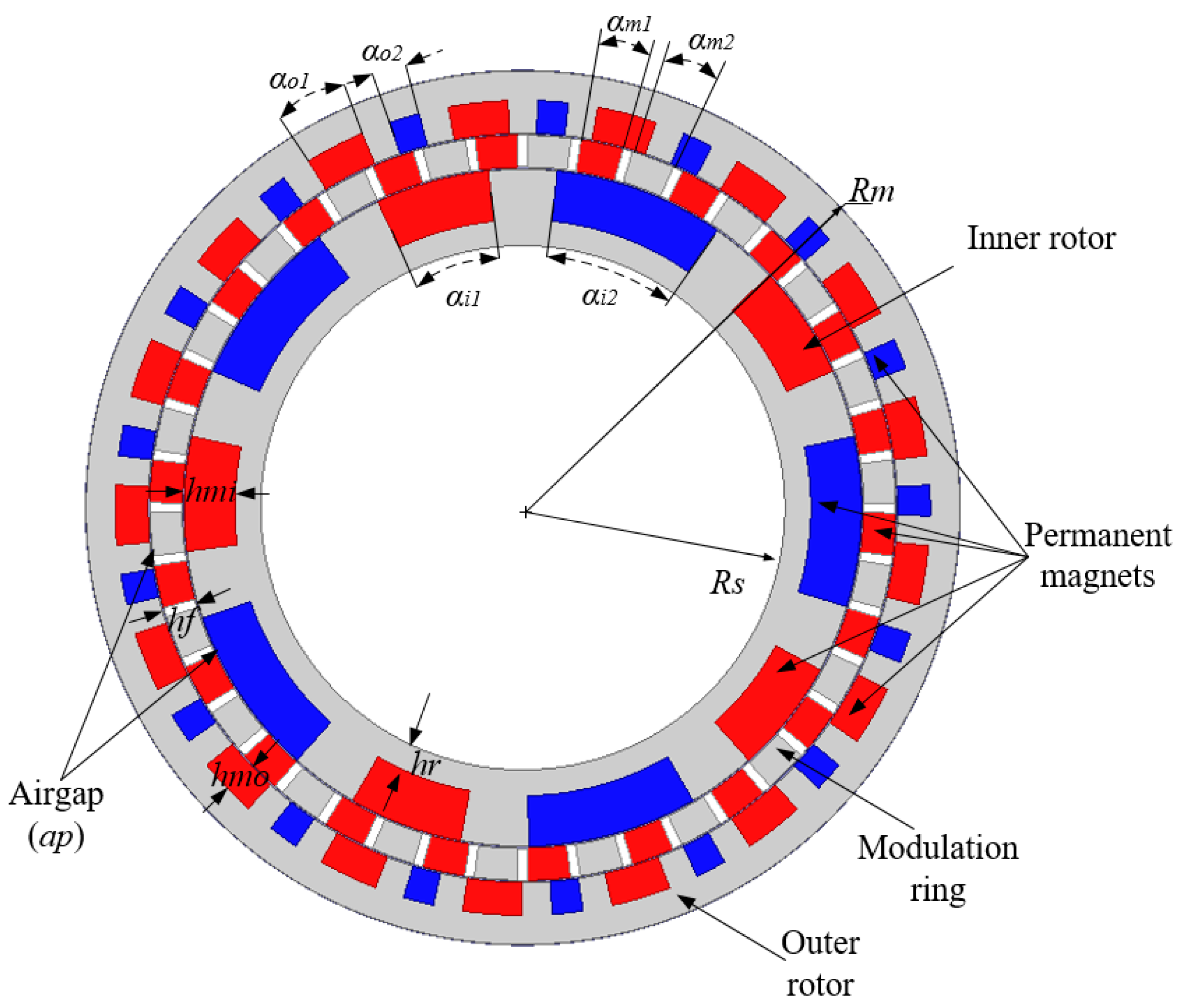
Figure 1. Three kinds of rotor arrays: (a) bipolar PM array (b) unipolar PM array (c) bipolar PM–ferrite array [23].
Energies 15 04963 g001
Figure 2. Three kinds of modulation arrays: (a) ferrite–air array (b) ferrite–PM array (c) ferrite–PM–air array [23].
Energies 15 04963 g002
Figure 3. Configuration of RMCSM-MG pattern.
Energies 15 04963 g003
Figure 4. Flux path of inner and outer rotor PM poles before modulation.
Energies 15 04963 g004
Figure 5. Torque ripple versus αi1 and αi2.
Energies 15 04963 g005
Figure 6. Torque ripple versus αo1 and αo2.
Energies 15 04963 g006
Figure 7. Cost value variation in each generation.
Energies 15 04963 g007
Figure 8. (a) Configuration of the original model. (b) Configuration of the optimized model.
Energies 15 04963 g008
Figure 9. Torque performance of the optimized and original model.
Energies 15 04963 g009
Table 1. Main parameters of the pattern of RMCSM-MG.
SymbolMeaningValue
piinner rotor pole pair number5
poouter rotor pole pair number17
mmodulation ferrite segments22
agairgap length0.5 mm
lgaxial length65 mm
hmiinner layer heightvariable
hfmiddle layer heightvariable
hmoouter layer heightvariable
hrinner rotor heightvariable
Rsinnermost radius60 mm
Rmoutermost radius105 mm
αi1angle of inner layer S polevariable
αi2angle of inner layer N polevariable
αm1angle of middle layer S polevariable
αm2angle of middle layer ferrite polevariable
αo1angle of outer layer S polevariable
αo2angle of outer layer N polevariable
μrrelative permibility1.044
Hcmagnetic coercivity−8.38 × 10⁵ A/m
Table 2. Parameter level design.
X1
(hmi)
X2
(hf)
X3
(hmo)
X4
(hr)
X5
(αi1)
Level 14 mm4 mm4 mm4 mm18°
Level 28 mm8 mm8 mm8 mm24°
Level 312 mm12 mm12 mm12 mm36°
X1
(hmi)
X2
(hf)
X3
(hmo)
X4
(hr)
X5
(αi1)
Level 118°60°/1760°/1760°/2260°/22
Level 224°120°/17120°/17120°/22120°/22
Level 336°180°/17180°/17180°/22180°/22
Table 3. L27 Taguchi orthogonal array and experimental results for objective function.
No.X1X2X3X4X5X6X7X8X9X10C(X)
1L1L1L1L1L1L1L1L1L1L147.39
2L1L1L1L1L2L2L2L2L2L269.29
3L1L1L1L1L3L3L3L3L3L3112.18
4L1L2L2L2L1L1L1L2L2L237.28
5L1L2L2L2L2L2L2L3L3L360.19
6L1L2L2L2L3L3L3L1L1L180.14
7L1L3L3L3L1L1L1L3L3L329.13
8L1L3L3L3L2L2L2L1L1L145.86
9L1L3L3L3L3L3L3L2L2L283.24
10L2L1L2L3L1L2L3L1L2L3112.43
11L2L1L2L3L2L3L1L2L3L113.08
12L2L1L2L3L3L1L2L3L1L271.91
13L2L2L3L1L1L2L3L2L3L139.62
14L2L2L3L1L2L3L1L3L1L256.42
15L2L2L3L1L3L1L2L1L2L361.95
16L2L3L1L2L1L2L3L3L1L2108.48
17L2L3L1L2L2L3L1L1L2L327.85
18L2L3L1L2L3L1L2L2L3L144.07
19L3L1L3L2L1L3L2L1L3L251.76
20L3L1L3L2L2L1L3L2L1L353.78
21L3L1L3L2L3L2L1L3L2L123.84
22L3L2L1L3L1L3L2L2L1L382.40
23L3L2L1L3L2L1L3L3L2L168.20
24L3L2L1L3L3L2L1L1L3L235.61
25L3L3L2L1L1L3L2L3L2L132.28
26L3L3L2L1L2L1L3L1L3L283.49
27L3L3L2L1L3L2L1L2L1L335.15
Table 4. Average analysis results.
X1X2X3X4X5X6X7X8X9X10
L162.7461.7466.1659.7560.0850.9033.9760.7164.6143.83
L259.5357.9758.4351.6253.1258.9357.7450.8757.3766.38
L351.8354.3949.5160.2060.8951.9482.3962.5152.1263.89
Table 5. Original and improved parameter value range.
ParameterOriginal Value RangeImproved Value Range
X1(hmi)[4 mm, 20 mm][4 mm, 8 mm]
X2(hf)[4 mm, 20 mm][4 mm, 8 mm]
X3(hmo)[4 mm, 20 mm][4 mm, 8 mm]
X4(hr)[4 mm, 20 mm][8 mm, 16 mm]
X5(αi1)[0°, 36°][30°, 42°]
X6(αi2)[0°, 36°][24°, 36°]
X7(αo1)[0°, 18°][120°/17, 240°/17]
X8(αo2)[0°, 18°][120°/17, 240°/17]
X9(αm1)[0°, 18°][0°/22, 120°/22]
X10(αm2)[0°, 18°][60°/22, 180°/22]
Table 6. Parameter level design of torque ripple function.
X1
(hmi)
X2
(hf)
X3
(hmo)
X4
(hr)
X5
(αi1)
Level 14 mm4 mm4 mm8 mm30°
Level 26 mm6 mm6 mm12 mm36°
Level 38 mm8 mm8 mm16 mm42°
X6
(αi2)
X7
(αo1)
X8
(αo2)
X9
(αm1)
X10
(αm2)
Level 124°120°/17120°/170°/2260°/22
Level 230°180°/17180°/1760°/22120°/22
Level 336°240°/17240°/17120°/22180°/22
Table 7. Average analysis results.
X1X2X3X4X5X6X7X8X9X10
SS0.040.110.250.031.771.871.741.680.680.81
PC(%)0.441.222.780.3319.720.819.418.77.579.02
Table 8. Parameters of the original model and optimized model.
ParameterOriginal ModelOptimized Model
X1 (hmi)11.54 mm7.9 mm
X2 (hf)7.31 mm8.0 mm
X3 (hmo)7.49 mm7.4 mm
X4 (hr)5.95 mm11.3 mm
X5 (αi1)19.5 deg35.8 deg
X6 (αi2)28.8 deg36.1 deg
X7 (αo1)8.5 deg10.4 deg
X8 (αo2)4.3 deg10.6 deg
X9 (αm1)6.6 deg0.0 deg
X10 (αm2)6.7 deg8.2 deg
Publisher’s Note: MDPI stays neutral with regard to jurisdictional claims in published maps and institutional affiliations.

