Remote Power Generation for Applications to Natural Gas Grid: A Comprehensive Market Review of Techno-Energetic, Economic and Environmental Performance

Abstract

The operation of natural gas grids requires electric-powered devices as data acquisition and control systems, surveillance and communication appliances, etc., often located in remote, unpopulated off-the-grid areas, where there is no personnel for surveillance, and maintenance costs are prohibitive. The literature on the power generating systems for these devices is limited to specific applications without a comparison between competing technologies, making their choice a difficult task for natural gas operators. This work presents a comprehensive up-to-date survey of market available technologies for remote power generation in the range of 20–1000 W for gas grid applications: thermoelectric generators, solid acid, direct methanol and solid oxide fuel cells, Stirling engines and microturbines. The work aims at sorting the technologies by techno-energetic, economic and environmental performance while providing specific technological characteristics and limitations. The results indicate well-defined ranges of power in which only some of the technologies are suitable and have very different efficiencies (3–30%). The capital cost of equal power technologies is similar (EUR 5000–30,000) and roughly linear with power (34.8P_el + EUR 6553), whereas operation costs (10–120 cEUR/kWh) and lifetime (0.5–20 yr) significantly depend on the technology. The indications of this review may constitute helpful guidelines to choose properly power generation systems for remote applications.

1. Introduction

The transmission and distribution gas grid makes use of several “small” (say below a few hundreds Watts) electric-powered applications located in geographically dispersed, remote, unpopulated, off-the-grid areas. Depending on the relative position in the gas system, these applications are broadly grouped into upstream and midstream ones [1,2,3]. Upstream refers to all facilities for production and stabilization of gas, including wellhead and well, i.e., on top of the actual gas well leading down to the reservoir; midstream is related to pipeline networks and gas-treatment systems.

The types, power levels and operation modes of these electric loads are briefly summarized in the following.

• Power supervisory control and data acquisition (SCADA) systems and remote terminal units (RTUs). The former are control system architectures comprising software and hardware elements that allow monitoring the wellhead or the pipeline by measuring, recording and transmitting data. RTUs are the part of the SCADA system which interfaces the metering equipment (i.e., telemetry units, flow meters, gas analyzers, leak detection sensors and valve setting monitor) to the rest of the SCADA system. The power requirement of SCADA systems/RTUs is on average between 5 and 20 W, and the energy consumption is 120–480 Wh per day, as they are operated continuously.
• Valve automation. It refers to all systems able to shut down the pipeline in the event of a safety concern (emergency shutdown (EDS) systems) [4,5] or to release, dose, distribute or mix fluids [6]. The actuation of the valve might be direct via a linear electric motor, or it may require a low-power DC pump. In both cases, the power demand is only required when the valve is actuated, but the high inrush current at startup results in relatively high power. The power levels of these devices are very different depending on the application, and range from a few tens up to a thousand Watts.
• Impressed current cathodic protection (ICCP). It is used to reduce or eliminate corrosion phenomena for buried or submerged metallic pipelines and producing gas wells casings [7,8]. An external direct current supplied from a power source cathodically polarizes the structure to be protected against corrosion. The anodes are made of durable materials that resist wear or dissolution. Iron with 14% silicon, carbon, and graphite are some commonly used anodes for pipeline protection [9]. Typical powers of a ICCP unit fit the range 200–500 W, and the impressed current varies from 3 to 30 A to match the variable ground bed resistance (the current drastically increases in low resistive soils). ICCP systems absorb a constant power around the clock.
• Injection systems. Gas hydrates represent a severe operational problem in raw gas transmission lines because crystals may deposit on the pipe wall and accumulate as large plugs, causing flow reduction or even block with considerable damage to production facilities [10,11]. They are ice-like crystalline solids that are formed when water molecules arrange themselves in a cage-like structure around methane molecules [12]. The most widely used method to prevent hydrate formation is to inject via pumps chemical additives in the gas stream, such as methanol, ethylene glycol, or triethylene glycol. A second typical application of injection system refers to the gas odorant, which is diluted in the gas stream for safety purposes. The required power of these systems is in the interval 10–50 W [13].
• Security and surveillance systems. It includes cameras and motion sensors to protect pipelines and sensitive infrastructures from thief and vandalism, located in remote, off-grid areas. The power requirement is on average between 25 and 100 W, and the energy consumption is 600–2400 Wh per day.
• Communication systems. They are broadly referred to as data transmission apparatuses for critical communications and emergency shutdown systems. These devices need a reliable backup power source and are particularly relevant for un/manned offshore platforms, which are operated in harsh environmental conditions. The power requirement ranges from 10 to 30 W.

Table 1. Average power requirements of electric powered applications in the gas transmission/distribution grid.

	Pel (W)
SCADA systems/RTUs	5–20
valve automation	10–1000
ICCP	200–500
injection systems	10–50
security and surveillance systems	25–100
communication systems	10–30

reports the power requirements of the above applications.

In addition, the growing penetration of the industrial Internet of Things (IIoT) in every level of the natural gas sector from wellheads, pipelines, terminals to local networks along with the diffusion of green gases (i.e., biomethane and hydrogen produced from renewable energy sources) is dramatically increasing the amount of small electric-powered devices that acquire data and use information to make real-time decisions autonomously [14,15,16]. For instance, cloud-based advanced analytics applied to transportation networks can be used to track and efficiently manage thousands of kilometers of pipelines, analyze the flow history to improve volume/pressure forecasting algorithms [17], detect leakages [18,19] or illegal tapping, reducing unnecessary downtime [20]. At a local level, IIoT applications allow creating local natural gas smart grids in the existing distribution infrastructure [21]. This requires instantly managing and regulating multiple, discontinuous and bidirectional flows coming from different resources located at multiple decentralised injection points and with different properties (natural gas, biomethane or hydrogen). In this complex scenario, maintaining the balance and structure of the entire network demands for a real-time and widespread monitoring of the gas distribution grid by sensor networks.

Finally, it is worth recalling that the natural gas industry widely uses pneumatic devices driven by the natural gas pressure where electric power is not available [22]. Pneumatic devices convert the enthalpy in the pressure form into useful work to power valve or liquid level controllers, pressure regulators and pumps. After expansion, the natural gas is vented into the atmosphere with severe negative effects on the environment, because of its very high greenhouse warming potential (GWP = 84). Methane emissions from pneumatic devices are one of the largest sources of vented methane emissions from the natural gas industry: 51 billion cubic feet (Bcf) per year in the production sector, 14 Bcf per year in the transmission sector and <1 Bcf per year in the processing sector [23]. The replacement of pneumatic devices with electric powered ones is one of the options to limit methane emissions, thereby reducing the impact on the environment and achieving significant savings [24].

An obvious possibility to power the aforementioned devices is to run the grid line to the site where the applications are installed. However, this solution is either technically unfeasible due to the long distances from the existing grid connection point, or economically not viable because of the high capital costs and service charges with respect to the small powers drawn from the grid. Moreover, in developing countries, the power grid reliability/resilience is a serious concern, being often below the requirements of many applications due to voltage sags, blackouts, overloads, etc. [25].

Photovoltaic and lead acid battery-based systems are a market viable option. However, being site dependent, their usage might be ineffective in locations where the solar panels productivity is limited (e.g., scarcity of daylight, snow over the panels, and shading) because the stored energy might be insufficient to cover the power demand. Furthermore, the capacity and lifetime of battery banks are significantly reduced by the extreme cold/hot temperatures often reached in gas production and transportation sites [26]. Finally, photovoltaic panels are prone to theft and vandalism [27].

In brief, the gas transmission/distribution grid demands for reliable small power generating devices to be operated in remote, geographically dispersed, unattended and often environmentally harsh areas. The choice of the power generating device is not straightforward because it should consider several concurrent aspects, such as energetic performance, reliability, costs, and environmental impact, in addition to all constraints in the location where they are installed (low temperature at startup, corrosive environment, theft risk, etc.). An analysis considering all these aspects for the wide variety of power generating devices to obtain choice criteria is missing in the literature.

The main goal of this review is to provide a comprehensive, consistent and up-to-date quantitative picture of technical, economic and environmental aspects of the commercially viable competing technologies for remote power generation in the range 20–1000 W for gas grid applications. The comparison of the technologies with respect to different metrics coupled with the examination of their specific technological characteristics and limitations allow drawing proper guidelines for their choice. To this aim, an extensive worldwide market survey among several companies in remote power solutions was performed. The data for the analysis are the result of public datasheets reworking or personal communications from the manufacturers.

The collection of data from actual applications and their critical comparison within a common and consistent framework, despite the very different nature of the several power generating devices, allow to get a novel picture of all the different market-viable technologies for small power generation.

The structure of the paper is as follows. At first, Section 2 presents a comparative technical analysis including thermal/power levels, nominal efficiency, performance derating over time and with environmental conditions and lifetime. Section 3 analyzes the economic aspects as the initial capital cost and the operation and maintenance costs. Finally, Section 4 discusses the environmental impact of each technology in terms of exhaust and noise emissions. Inasmuch as this work is aimed at a interdisciplinary audience, the working principle, main constructive features and peculiar aspects of the remote power devices are reported in Appendix A.

2. Techno-Energetic Analysis

This section first analyzes and then compares all the technologies for remote power generation (the working principles and the basic features of these technologies are presented in Appendix A).

The considered technical parameters are thermal/power levels, nominal efficiency, performance derating over time and with environmental conditions and lifetime (Section 2). In the following, the technical analysis of TEGs (Section 2.1), FCs (Section 2.2), FPSEs (Section 2.3) and MTs (Section 2.4) is presented. Subsequently, the above technologies are directly compared (Section 2.5).

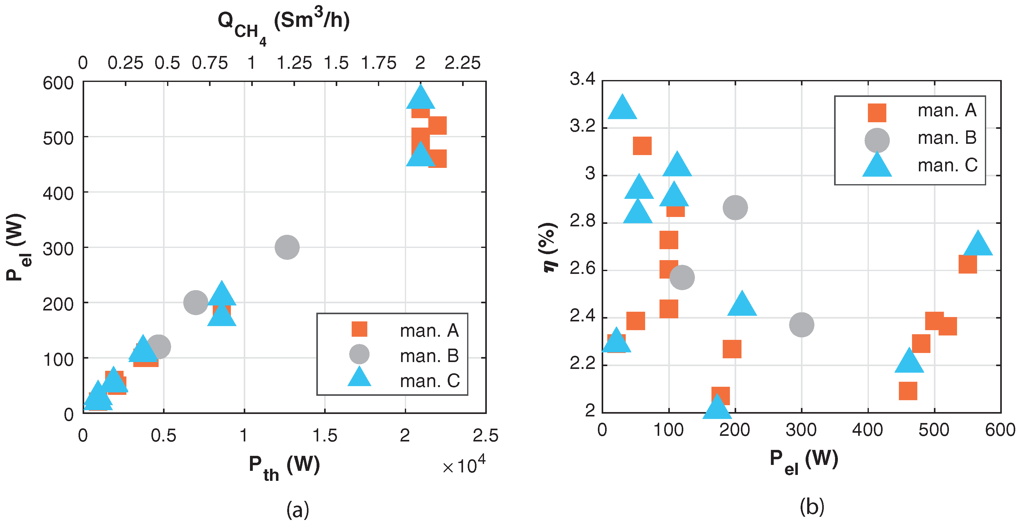
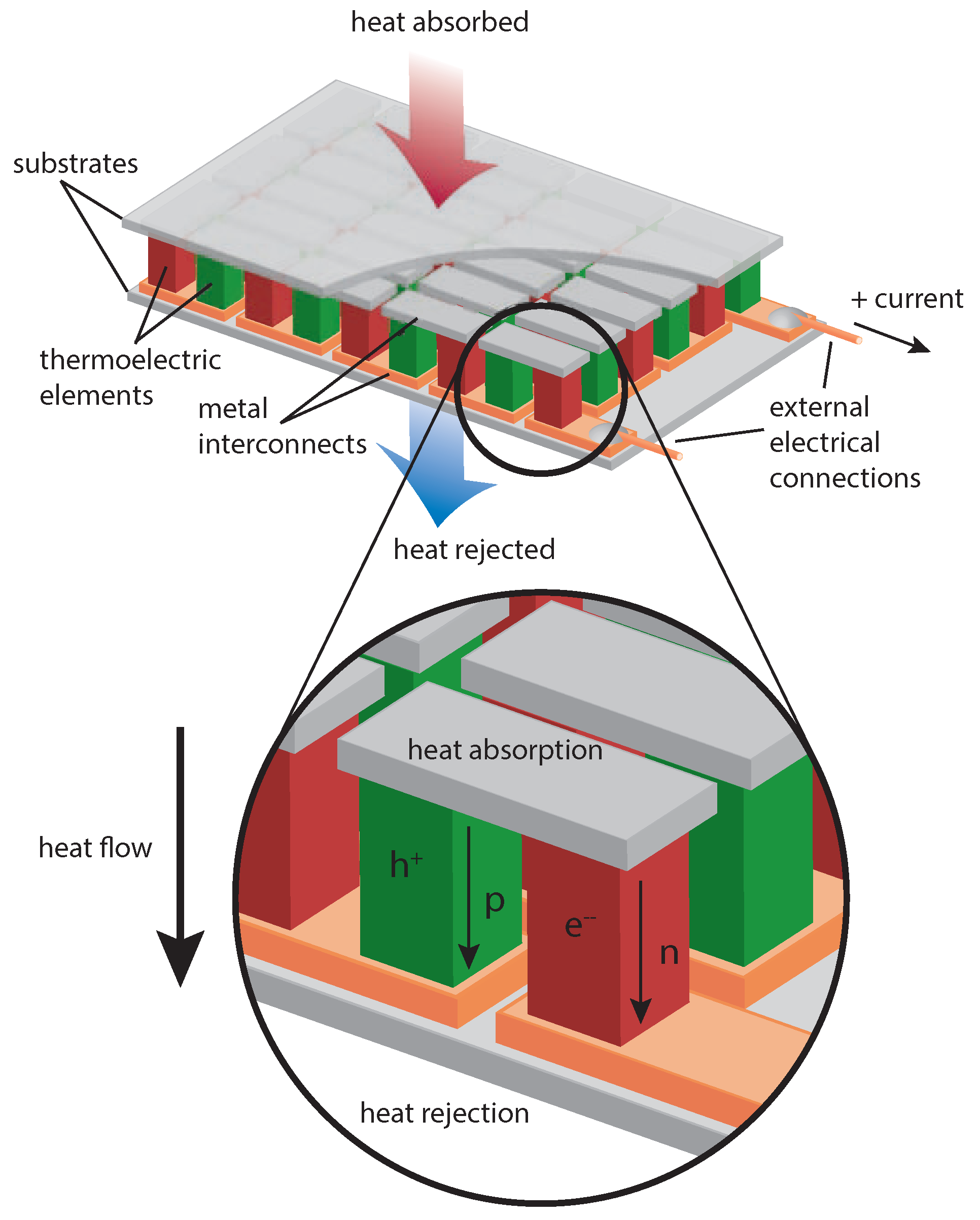
2.1. Thermoelectric Generators (TEGs)

Figure 1a shows the power levels of TEGs from three manufacturers as a function of thermal power and corresponding natural gas volumetric flow rate. The known value of fuel consumption and the higher heating value (37.7 MJ/Sm${}^3$ [28]) are used for the calculation of the thermal power. The electric power referred to an ambient temperature of $20{}^{°}\mathrm{C}$ (i.e., nominal conditions) ranges from 15 to 550 W. Correspondingly, the required thermal power is between a little less than 1 kW up to almost 22 kW, and it is made available by the combustion of a natural gas flow rate equal to 0.09 Sm${}^3/$h (2.1 Sm${}^3/$d) and 2.1 Sm${}^3/$h (50.4 Sm${}^3/$d), respectively. Note that points with the same thermal power input, but slightly different electric power output are reported: they refer to the same TEG operated at a different output voltage. The output voltage is usually standardized at 12 or 24 VDC, but different levels (i.e., 14 or 48 VDC) are also possible depending on the application. Depending on the TEG size, the minimum supply pressure is in the range 70–100 kPa, and the maximum one lays between 170 and 345 kPa. Thus, the natural gas flow rate withdrawn from the network must be throttled before feeding the TEG.

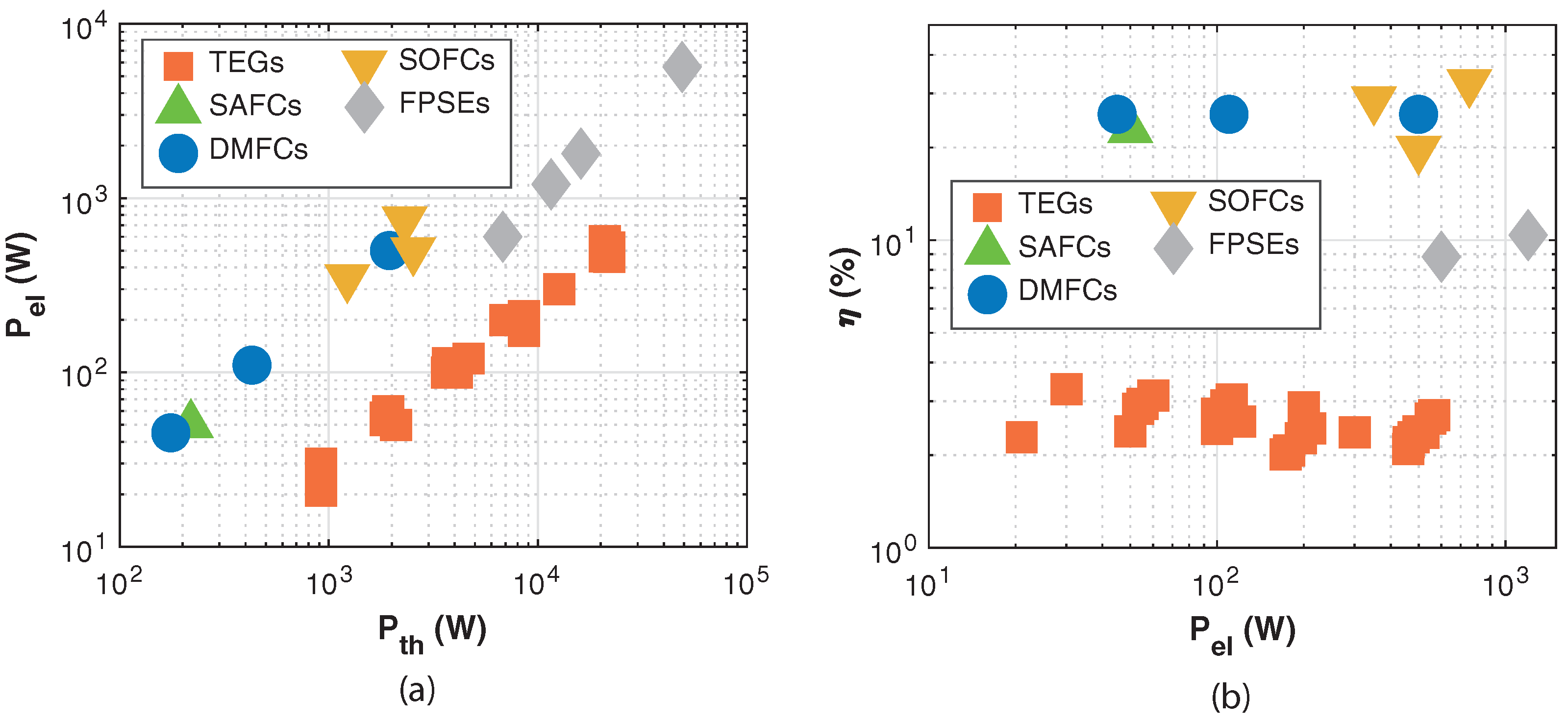
Nominal efficiencies, i.e., net electric-to-thermal power ratio in nominal conditions, are collected in Figure 1b. Efficiency values are apparently very low and fit the narrow range 2–3% on average. The comparison of the efficiency at different power levels highlights that TEGs do not suffer from the scale effect. The performance levels of smaller size TEGs are similar or even a bit better than those of higher size, allowing for a scaling-down without penalties.

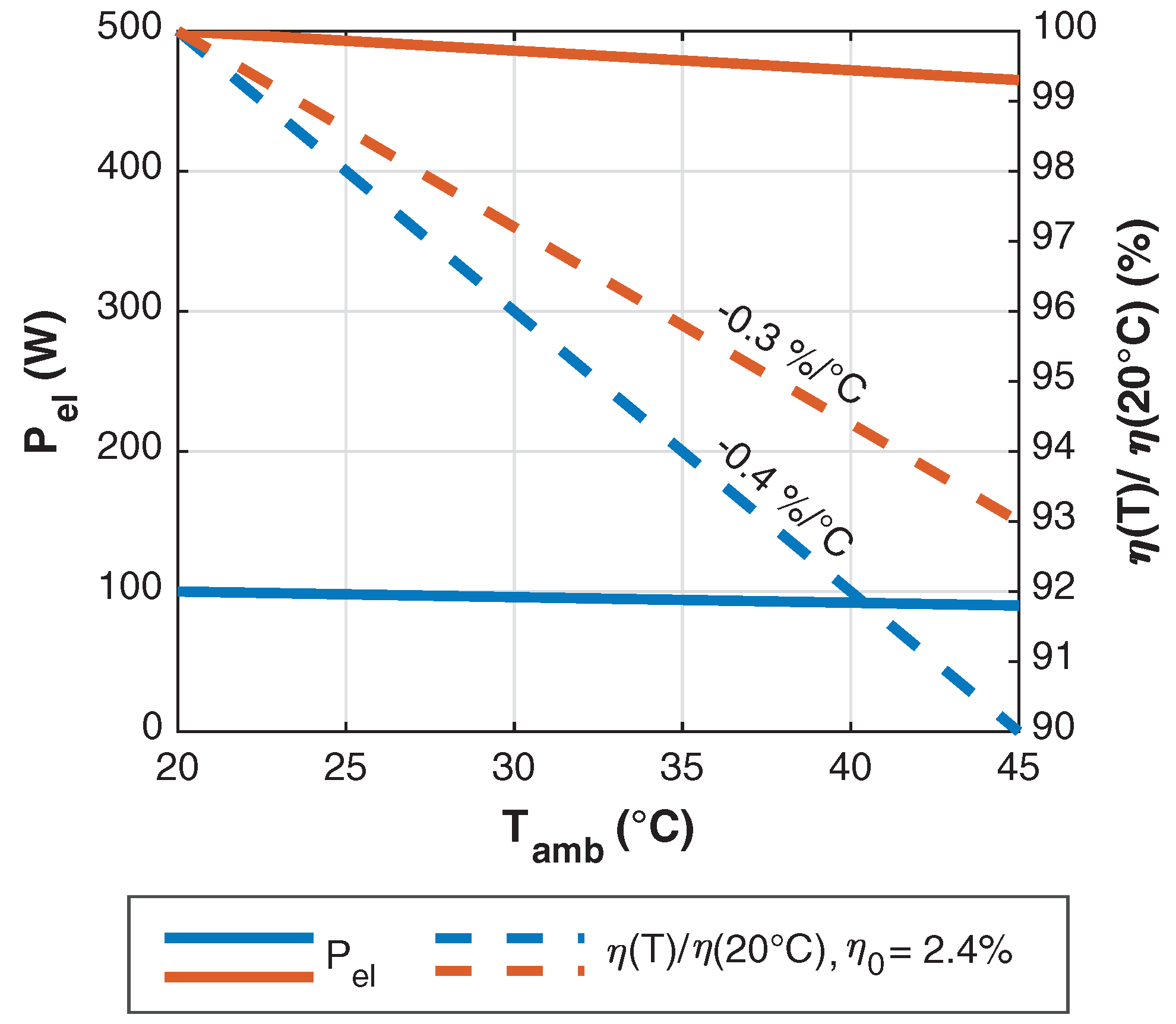
Figure 2 refers to the impact of the ambient temperature: the higher the ambient temperature, the higher the TEG hot side and, in turn, the lower the power output and efficiency (see Appendix A.1). As a first approximation, a linear relationship between power and ambient temperature can be assumed and typical average power derates are −0.4 and −1.4 W/${}^{°}\mathrm{C}$ above $20{}^{°}\mathrm{C}$ for 100 and 500 W sized TEGs, respectively. Correspondingly, the relative efficiency/power derates with respect to the nominal efficiency/power (i.e., slope of the P(t)/P(0) or $\eta \left(t\right)/\eta \left(0\right)$ dotted lines in Figure 2) are −2.8 and −4% 10${}^{°}\mathrm{C}$ above $20{}^{°}\mathrm{C}$. This means, for instance, that a nominal 100 W TEG operated at $40{}^{°}\mathrm{C}$ produces only 92 W, that is, its efficiency lowers to 92% of the nominal one. The minimum ambient temperature allowed for TEG operation is $-40{}^{°}\mathrm{C}$ due to limitations imposed by the conditioning electronics.

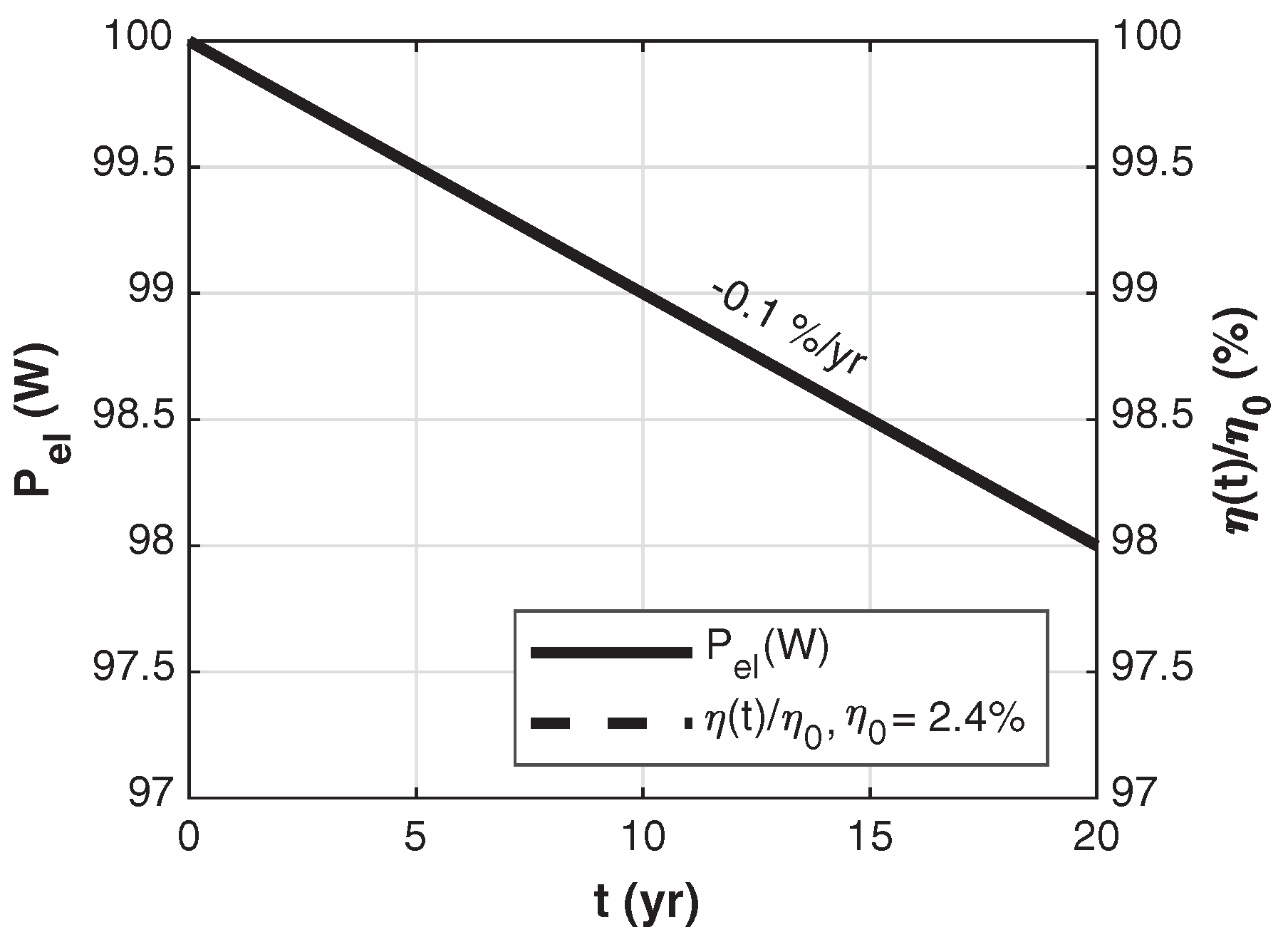
The aging effect, i.e., the performance decay in time is reported in Figure 3 for a typical 100 W TEG. The decrease in power output is very limited, equal to −0.1 W/yr (≈−0.01 W/1000 h), mainly due to the leaching away from one another of the p-n junction materials. The average relative efficiency/power derate is −0.1% /yr (curves in Figure 3 are overlapped).

The lifetime of the power unit (which is the most expensive part of the TEG) lasts for 20 years, even in harsh environments, being hermetically sealed in stainless steel cabinets. Moreover, the relatively small and unobtrusive size of TEGs permit the mounting inside security shelters to prevent theft and vandalism; unsheltered operation on pole mount or bench stand are possible for the smallest sizes, as well.

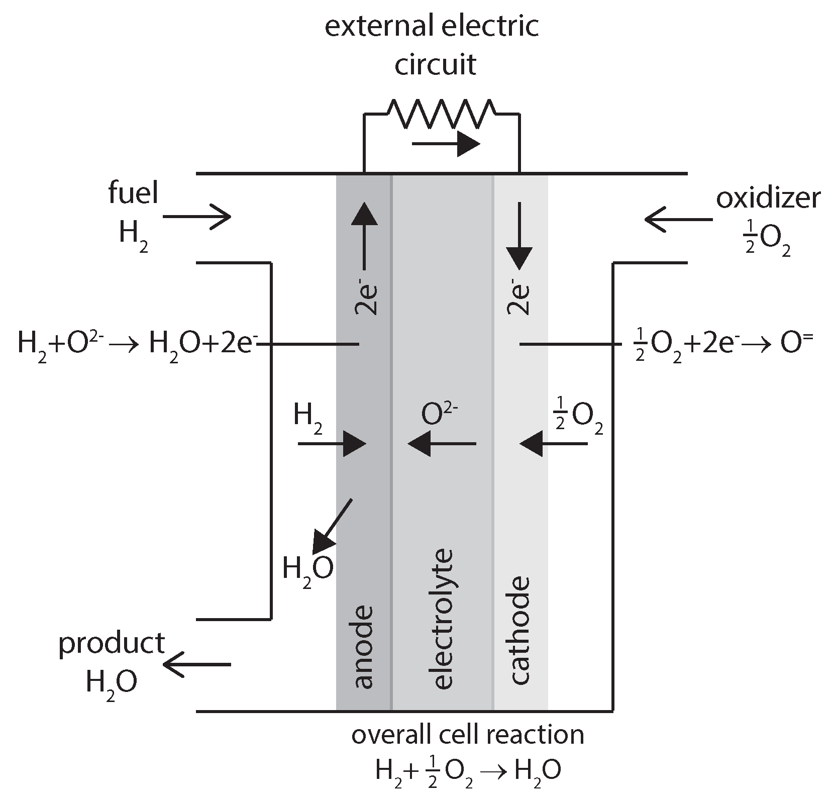
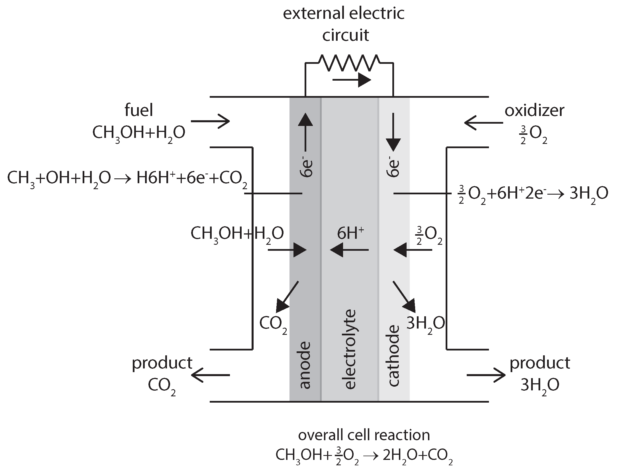
2.2. Fuel Cells (FCs)

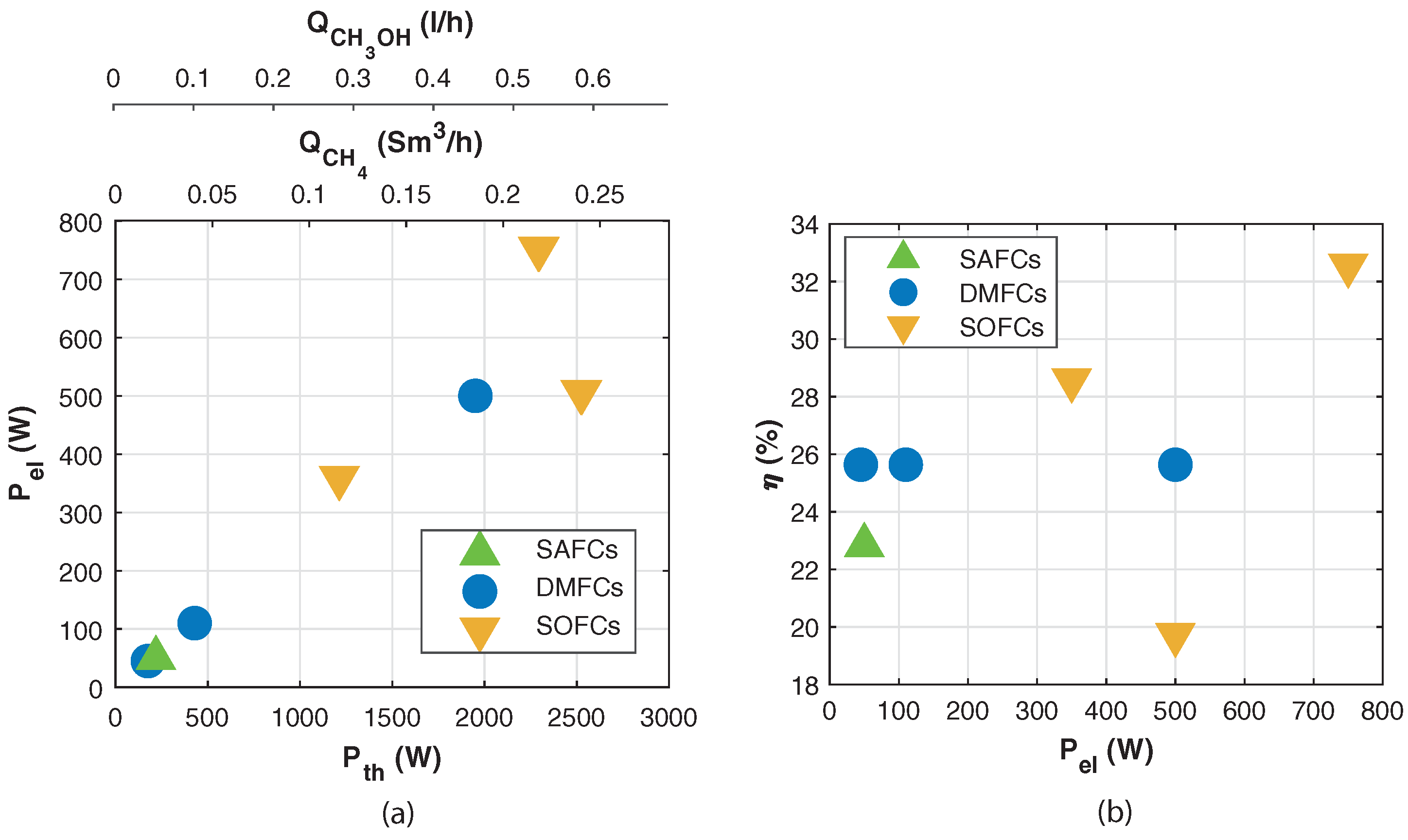
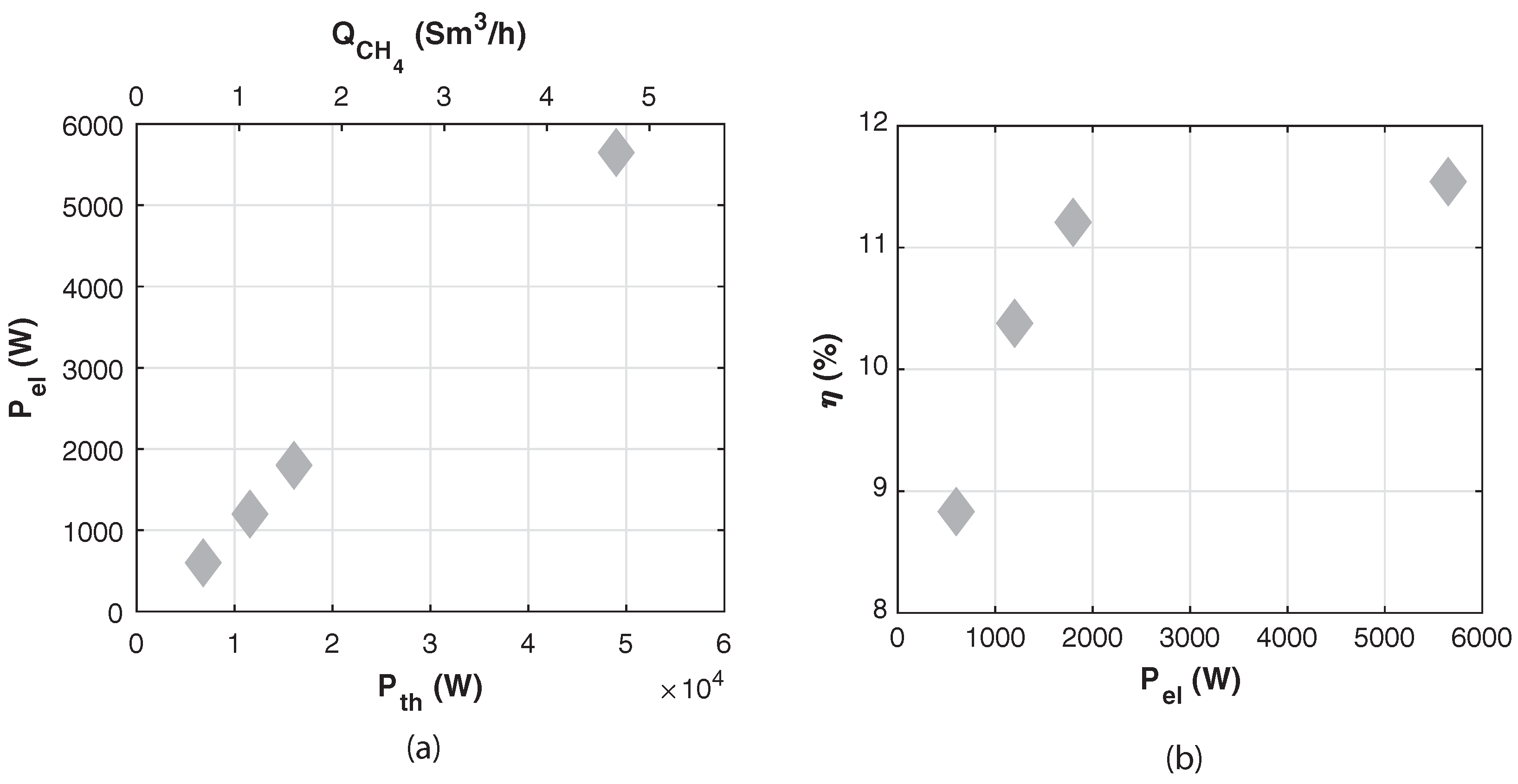
Figure 4a shows the power levels of fuel cells and the corresponding known fuel consumption of natural gas for SOFCs and methanol for SAFCs or DMFCs. The heating values for the calculation of thermal power are 37.7 MJ/Sm${}^3$ and 19.7 MJ/Kg, respectively [28]. The output electric power ranges from 45 to 750 W: SAFCs and DMFCs cover approximately the lower half of the interval, whereas SOFCs cover the upper one. The thermal power fits the interval 175–2000 W (0.04–0.45 L/h, 1–11 L/d of methanol) for methanol fueled FC and 1200–2500 W (0.12–0.22 Sm${}^3/$h, 2.8–5.3 Sm${}^3/$d of natural gas) for SOFC.

Efficiency is reported in Figure 4b. For the sake of consistency with the other technologies, they are calculated as the net electric power-to-thermal power ratio and range from 20% to almost 33%, regardless of the size. It is worth observing that the seemingly low efficiency of SOFCs is the result of a design choice: the reforming is external to obtain a simpler water drain and, in turn, a more robust device.

The rated voltage is 12/24 VDC, depending on the user characteristics. The ambient temperature does not significantly affect the FC performance and could span the range −20 to +$50{}^{°}\mathrm{C}$ for DMFCs and SOFCs. SAFCs can be operated, even in colder environments up to $-40{}^{°}\mathrm{C}$, but still require a minimum start-up temperature around $-20{}^{°}\mathrm{C}$. To the authors’ knowledge, there are not commercially available FCs rated to operate in potentially explosive atmospheres. However, the protection of all the possible sources of ignition (sparks, flames, electric arcs, high surface temperatures, electromagnetic waves, etc.) and the enclosing of the system in a flameproof structure to physically isolate it from the potentially explosive atmosphere might allow FCs to comply with ATEX directive [29].

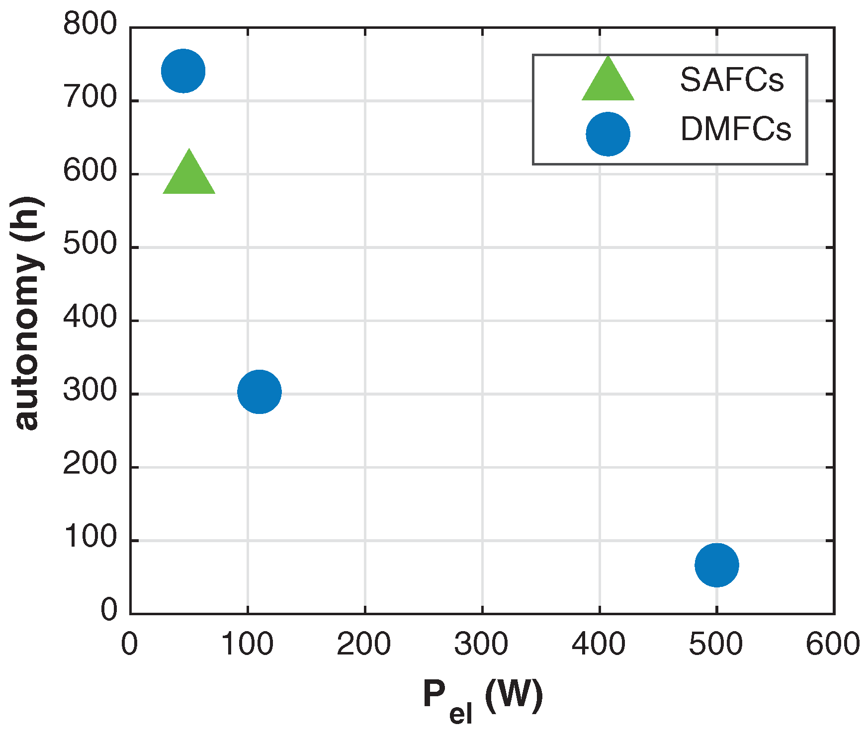
For methanol-fueled SAFCs and DMFCs, the fuel consumption rate is related to the autonomy of the fuel cell by the methanol tank capacity. Figure 5 shows the hours of continuous operation as a function of the output electric power for a 30 L tank capacity. The calculated time based on the declared fuel consumption rates is less than linearly proportional to the tank capacity and ranges from more than 700 h for 50 W devices, down to less than 100 h to obtain 500 W. However, it should be borne in mind that (i) electric power demand is not constant, that is, the operation of power supply devices is intermittent and (ii) tanks up to hundreds of liters might be used, especially at well sites where space constraints are weaker.

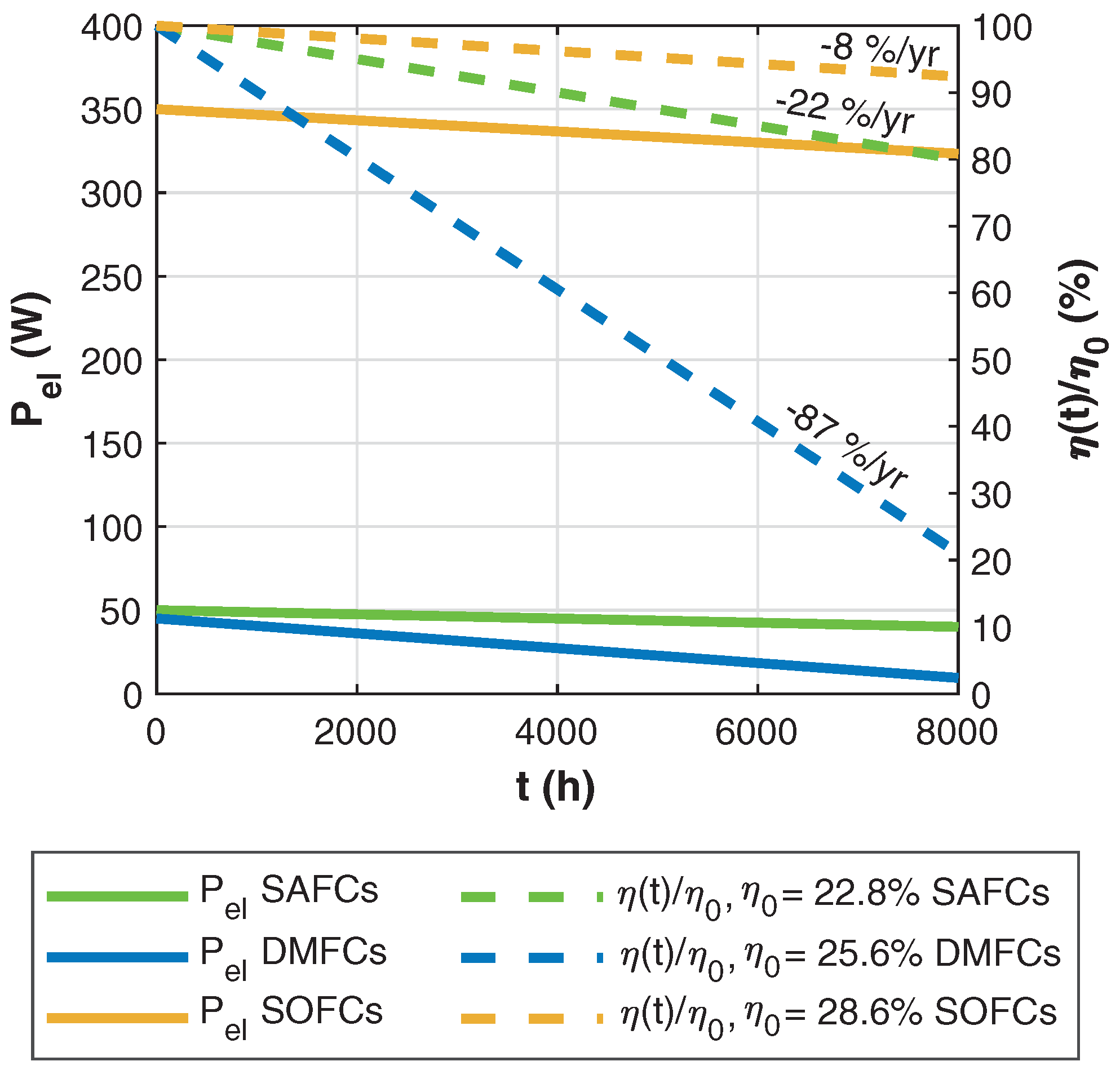
The fuel cell power degradation depends on both intrinsic characteristics and working conditions, such as start–stop cycle frequency, variation of the electric load, relative duration of the nominal power operation, etc. The aging effect on 350 W SOFC, 50 W SAFC and 45 W DMFC performance is shown in Figure 6. Power levels measured after 8000 h of continuous operation are used to estimate the reported linear trends. The average decrease in power output is very relevant for all the three considered FC types: −29 W/yr for SOFC, −11 W/yr for SAFC and −39 W/yr for DMFC. Correspondingly, the average relative derates of efficiency/power are −8%/yr, −22%/yr and −87%/yr.

Clear and consistent data on the lifetime of FCs systems are difficult to be collected from the manufacturers because of the following:

(i)

The definition of the lifetime end point is not unique and can be alternatively based on the change in the total resistance, output voltage or nominal power;

(ii)

In the actual fuel cell operation, the scheduled maintenance or even replacement of some components lengthen the real lifetime.

According to a definition by the US Department of Energy [30], a fuel cell reaches its lifetime when it loses 10% of its nominal power. Consequently, see Figure 4, the lifetimes of SOFCs, SAFCs and DMFCs are around 10,500, 4000 and 1000 h of continuous operation, respectively. However, this does not mean that after these intervals, FCs are to be completely replaced. In fact, SOFCs manufactures state an actual stack service lifetime up to 4–5 years (35,000–44,000 h) of continuous operation, provided that maintenance related to natural gas impurities (mercaptan removal) is regularly done and some components as gas pumps are replaced after 1000 operational hours. As for SAFCs, some of the components are only rated for a mean time between failure of 10,000 h, and therefore 8000 h are generally warranted by the manufacturer.

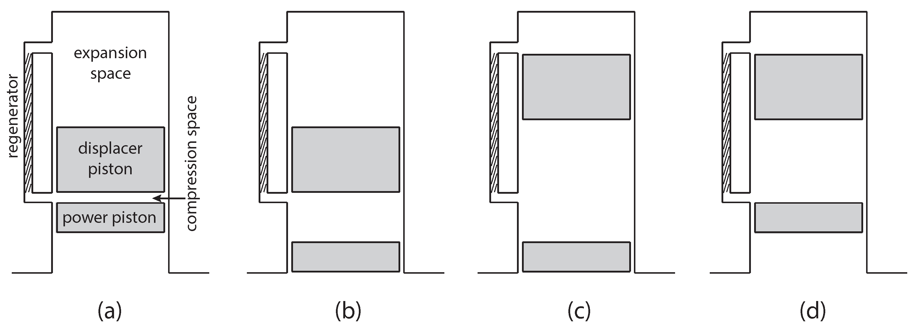
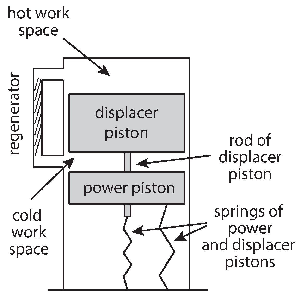
2.3. Free Piston Stirling Engines (FPSEs)

The power levels of FPSEs and the corresponding natural gas consumption are shown in Figure 7a. For the sake of completeness, also engine sizes higher than those suitable for remote power generation in the natural gas sector are included. Electric power spans a wide interval ranging from 600 to almost 6000 W. The corresponding natural gas flow rates are 0.65 Sm${}^3/$h (16 Sm${}^3/$d, 6.8 kW) and 4.7 Sm${}^3/$h (112 Sm${}^3/$d, 49 kW), which can be supplied at 20–345 bar. As a result, the nominal efficiency calculated as electric-to-thermal power ratio (HHV = 37.7 MJ/Sm${}^3$) is around 10.5% on average, and almost 9% for the 600 W size (see Figure 7b). Depending on the application, the electric output can be 120/240 VAC at 60 Hz or low voltage 12/24 VDC with the use of a converter. The possibility to achieve relatively high voltages is advantageous for cathodic protection application because it permits to maintain a proper current level also in high resistivity ground beds, without the need to put more generators in series.

The FPSEs performance is not significantly affected by the ambient temperature. The allowed operating temperature is between −25 and $50{}^{°}\mathrm{C}$, whereas the minimum startup temperature is $-15{}^{°}\mathrm{C}$. Nevertheless, a low-temperature cold start package down to $-40{}^{°}\mathrm{C}$ is available for extreme environmental conditions.

The altitude of the FPSEs installations affects the performance because it controls the ambient pressure and, in turn, the combustion air density: the higher the altitude, the lower the performance. For a 600 W sized SE, the average relative derate of efficiency/power is around 8% every 500 m above 1500 m.

The FPSEs power output is almost constant over time (quantitative data from on field measurements are not available). The lifetime order of magnitude is 10 years. The ordinary maintenance is less than one hour per year mainly to check coolant levels and air filter.

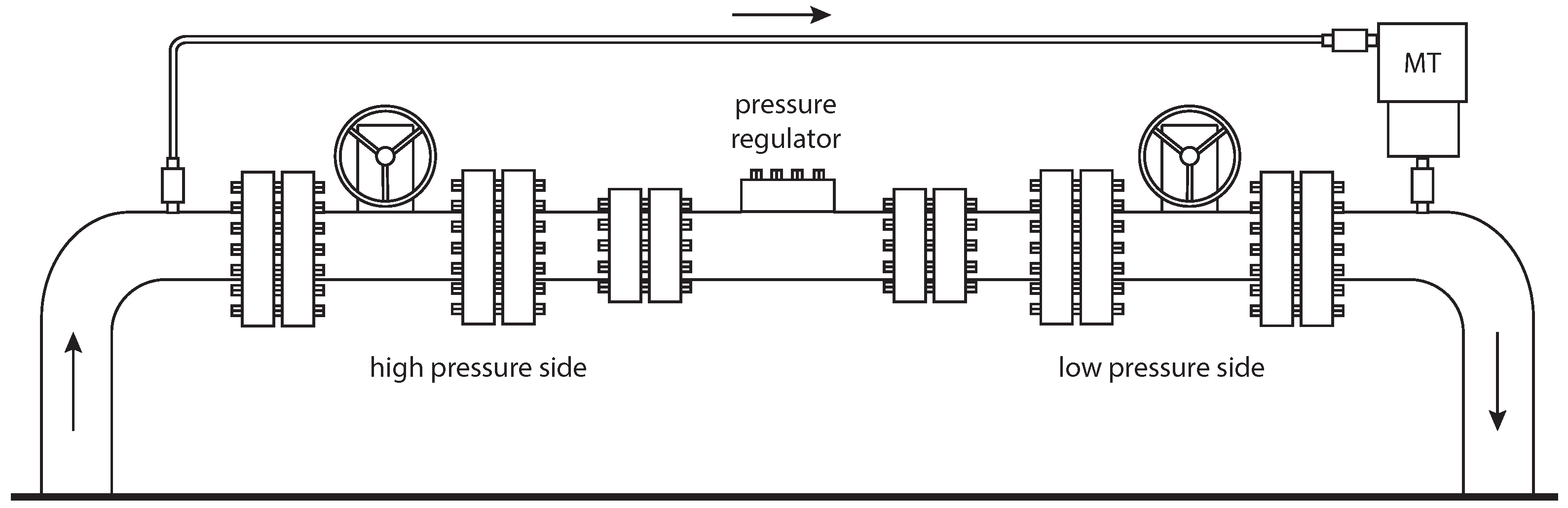
2.4. Microturbines (MTs)

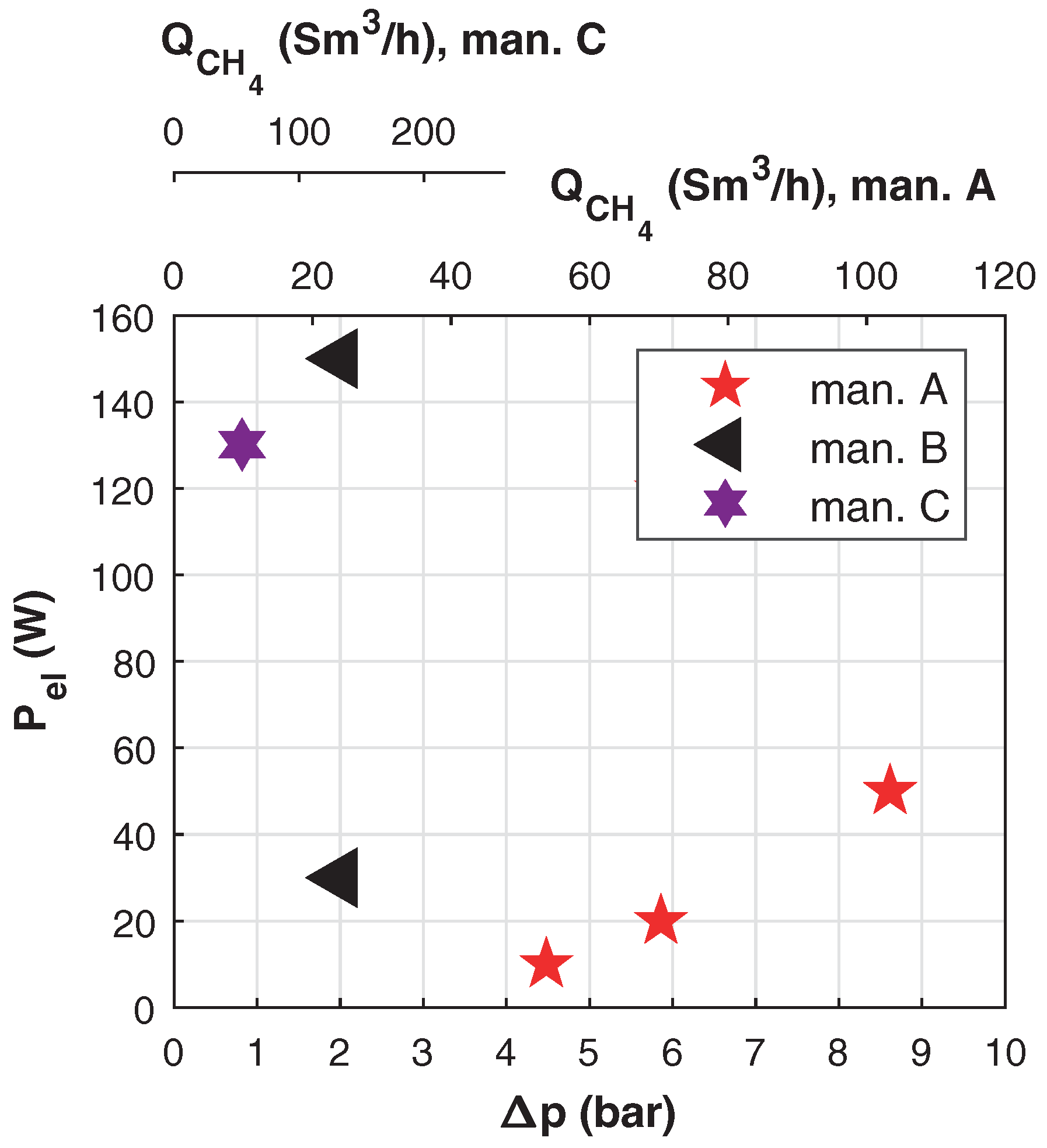
Figure 8 shows the power levels of MTs as a function of the pressure drop across them. These miniaturized turbines operate in parallel with station regulators and produce a few tens Watts, exploiting pressure drops of about 2–8 bar. The dimensions are very limited: for instance, the rotor diameters of the 30 and 150 W MTs in Figure 8 are 70 and 80 mm, respectively. The maximum inlet pressure depends on both the design choices and constructive aspects (e.g., robustness, seals, manufacturing technique, and coupling with the electric generator): it is 30–40 bar for the two models operating across a 2 bar pressure drop and 100 bar for the others.

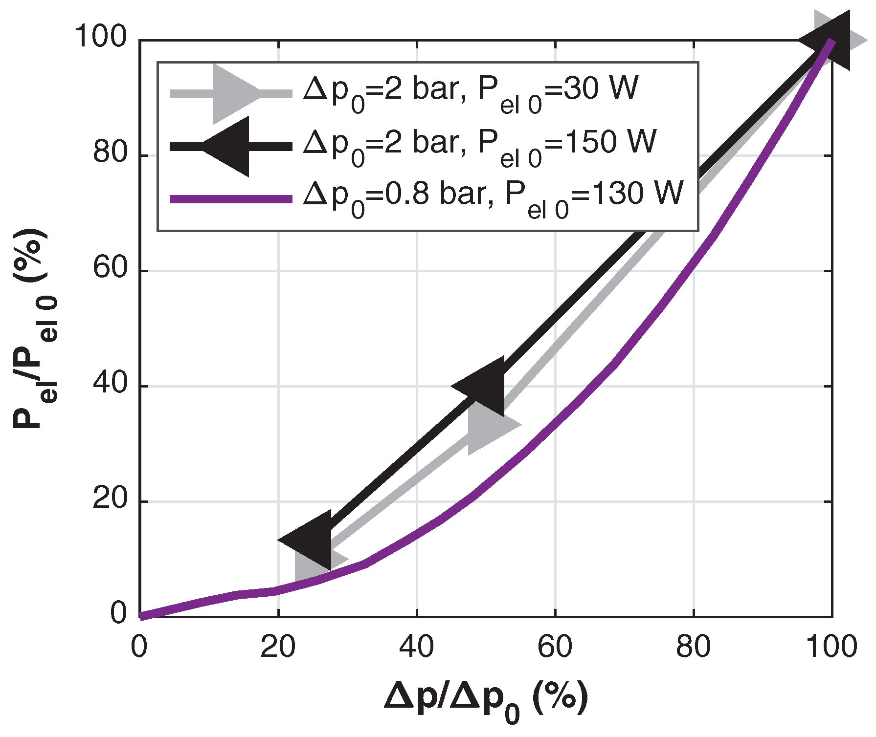
The operating parameters of the gas network are not constant over time: they change depending on the gas demand, the pressure distribution and, in turn, the mass flows through the network branches change. As a result, MTs are subject to variable boundary conditions imposed by the local gas network operation. The pressure drop across the rotor ($\mathsf{\Delta }p$) might be lower than the design one ($\mathsf{\Delta }{p}_0$), so reducing the output power. Figure 9 shows the relationship between the actual-to-nominal power ratio and actual-to-nominal pressure drop ratio for two MTs of different nominal power, namely 30 and 150 W. The relative power decreases almost linearly with the relative pressure drop: the power derate is, at first approximation, size independent and equal to 12% every 10% pressure drop reduction.

The standardized output voltage of MTs is 12/24 VDC. Since MTs always operate in potentially explosive atmospheres, they are class I, division 1, group D certified (North America) or ATEX Zone 1, II 2G Ex mb c IIC Tx X Gb (Europe). MTs might be operated in the thermal range −20–$40{}^{°}\mathrm{C}$ and are unaffected by whether conditions or dust build up. Maintenance work is negligible and the average lifetime is 7 years.

2.5. Comparative Technical Analysis of the Different Technologies

Figure 10a shows at a glance the intervals of application of the different technologies in the thermal–electric power plane (MTs are not reported, but are considered in the following analysis). TEGs cover the widest thermal/electric power intervals (1000–20,000 W and 20–600 W, respectively) to fulfill, together with MTs, the very low power demands (say less than 50 W down to 10 W). On the other hand, FPSEs are suited for the most power-consuming applications, above 1000 W, with a ten times larger thermal input. SOFCs cover the upper half of FC power domain (350–900 W), whereas DMFCs and SAFCs generally meet a power demand less than 100 W. Accordingly, three power thresholds can be broadly identified: below 50 W TEGs or MTs are necessarily to be chosen, between 50 and 600 W TEGs and FCs are both viable options, and over 600 W SOFCs or FPSEs are to be preferred.

Nominal efficiencies are reported in Figure 10b. Depending on the technology, three distinct and non-overlapping efficiency intervals can be clearly identified. TEGs have definitely the lowest efficiencies in the range 2–3%, FPSEs are around 10% and FCs achieve the highest efficiencies in the range 20–30%.

However, the comparative analysis of performance cannot disregard the efficiency decay over time and, in turn, lifetime and the impact of environmental/external conditions.

As for efficiency derate, TEGs and FPSEs have almost constant performance over time and are characterized by a relatively longer lifetime. The solid-state design of TEGs ensures trouble-free operation, and over 30 years of worldwide presence in power solutions for remote unattended areas make this technology the most reliable and field proven. Conversely, FCs applications for remote power generation in the natural gas sector are strongly hindered by very high power derates and resulting short lifetimes, quite unfit to face the required operation time of 5–10 yr, typical of gas grid applications.

As for the impact of ambient/external conditions, MTs are the option most dependent on external factors because of the strong influence on power output of the pressure drop imposed by the gas network. TEGs reduce the power output with the ambient temperature, may be installed in extreme climatic conditions and are not affected by salt spray, bird droppings or airborne contaminants. FCs and FPSEs are almost independent of ordinary ambient/external conditions, but FCs suffer of fuel impurities. All the considered technologies share the same maximum operating temperature, approximately $50{}^{°}\mathrm{C}$. TEGs and SAFCs are best suited to very cold climates down to $-40{}^{°}\mathrm{C}$, whereas DMFCs, SOFCs and FPSEs demand for minimum operating temperature around $-20{}^{°}\mathrm{C}$.

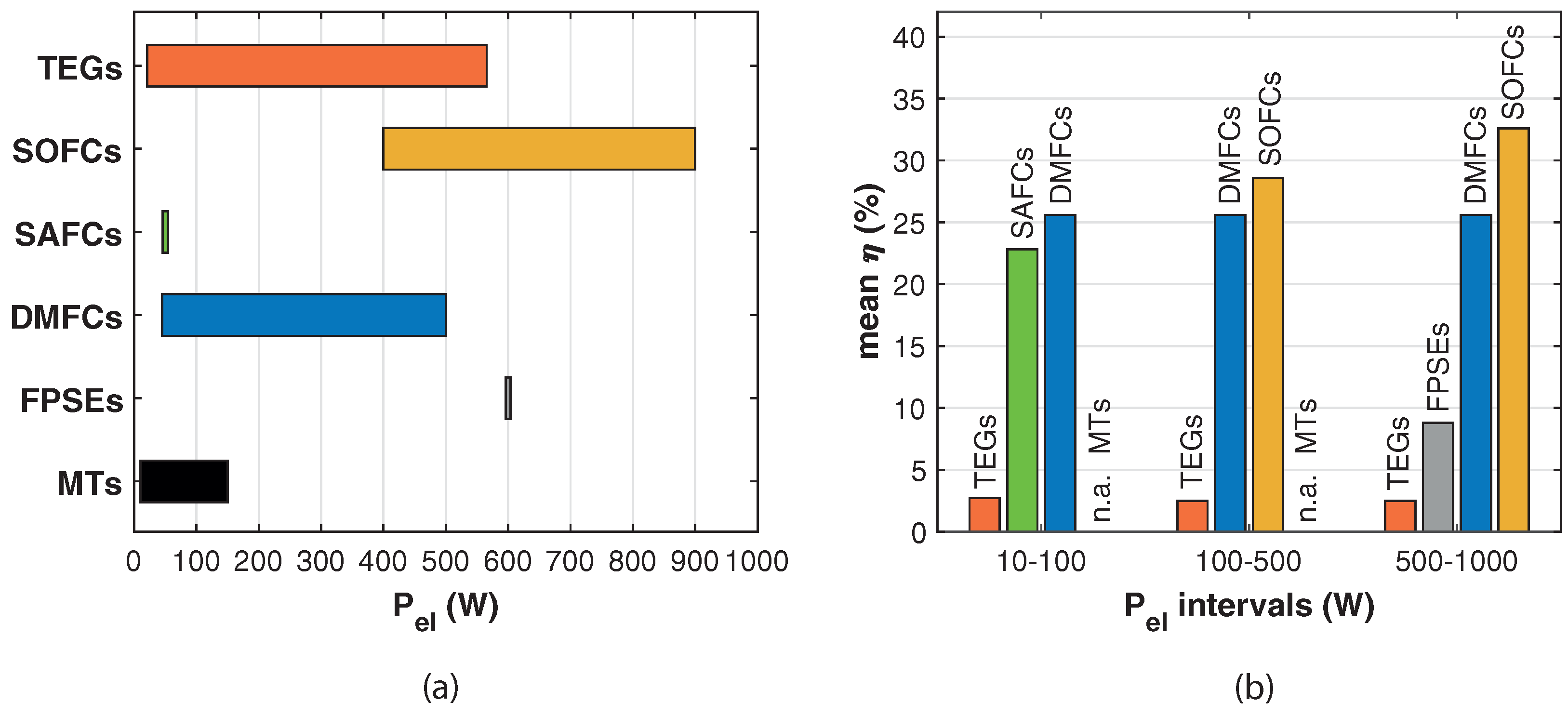
The infographics in Figure 11 show at a glance the main technical features of the devices. The bar chart in Figure 11a reports the electric power intervals covered by each technology below 1000 W. TEGs and DMFCs are available in almost equal and wide intervals, say 20–550 W, MTs fit the range 10–150 W, whereas the only available SAFC model is 50 W sized. SOFCs span the upper interval 350–900 W along with FPSEs (here, only the 600 W model is included because it is the only one below 1000 W).

Figure 11b shows the viable technologies in three power classes (10–100, 100–500 and 500–1000 W) sorted by the corresponding mean efficiencies. In the lower class, 10–100 W, the competing options in ascending order of efficiency are TEGs (2.7%) < SAFCs (22.8%) < DMFCs (25.6%) and MTs. In the intermediate class, 100–500 W, SAFCs are unavailable and SOFCs are usable; therefore, the resulting sorting is TEGs (2.5%) < DMFCs (25.6%) < SOFCs (28.6%) and MTs. In the upper class, 500–1000 W, MTs are not available but FPSEs are a further option, and hence TEGs (2.5%) < FPSEs (8.8%) < DMFCs (25.6%) < SOFCs (32.6%).

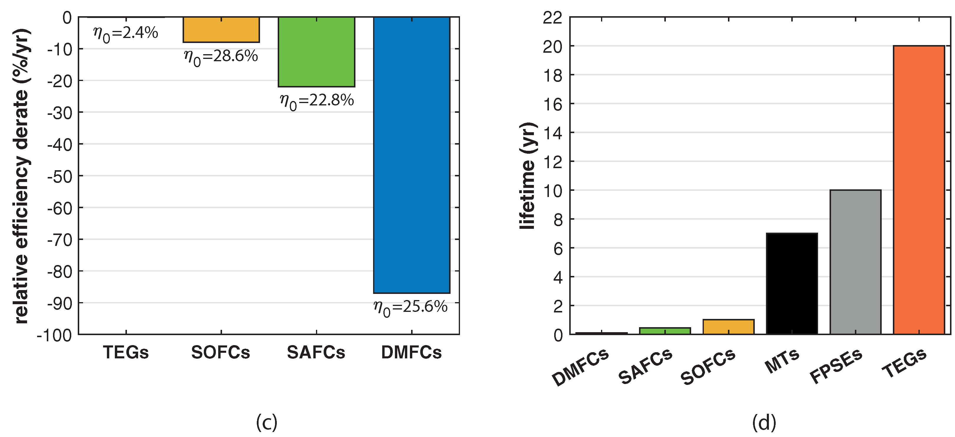
Figure 11c visualizes the relative efficiency derates (i.e., slopes of $\eta \left(t\right)/{\eta }_0$) for TEGs and FCs: the former (0.1%) is two orders of magnitude lower than the others (10%, 22%, 87% for SOFCs, SAFCs and DMFCs, respectively).

Finally, Figure 11d sorts all the technologies by the lifetime: the FCs lifetimes (defined as time to reach 90% of the nominal power) are much shorter (1000–10,000 h) than those of MTs (7 yr), FPSEs (10 yr) and TEGs (20 yr).

Table 2. Technical features of TEGs, SOFCs, SAFCs, DMFCs, FPSEs and MTs.

	TEGs	SOFCs	SAFCs	DMFCs	FPSEs	MTs
Pel (W)	20–500	400–900	50	45–500	600	30–150
Pth (W)	900–22,000	1225–2300	220	175–1950	6800	N.A.
$\eta$ (%)	2.3–3	26.5–32.5	23	25.5	8.8	n.a.
relative * efficiency/power derate (%/yr)	−0.1	−8	−22	−87	n.a.	n.a.
lifetime (yr or h)	20	10500	4000	1000	10	7
operating temperature (${}^{°}\mathrm{C}$)	−40 +45	−20 +55	−40 +40	−20 +50	−25 +50	−20 +60
min/max fuel supply pressure (kPa)	70–100/170–345	1.8/5	N.A.	N.A.	20/345	N.A./800–10,000

Note: N.A.: not applicable; n.a.: not available; * with respect to the nominal performance.

collects the main technical data of the technologies for remote power generation in the gas grid.

3. Economic Analysis

This section deals with the economic aspects of the different technologies for remote power generation in the natural gas sector. Similar to the above technical analysis (Section 2), economic data were collected from manufacturers in the year 2021. All data are reported in Euros (for the Euro to US dollar exchange rate: EUR 1 = USD 1.21). The considered economic parameters are capital and the operation and maintenance costs. In the following, the economic analyses for TEGs (Section 3.1) and FCs (Section 3.2) are presented. A brief direct comparison between the technologies, including some hints on FPSEs and MTs, ends the analysis (Section 3.3).

3.1. Thermoelectic Generators (TEGs)

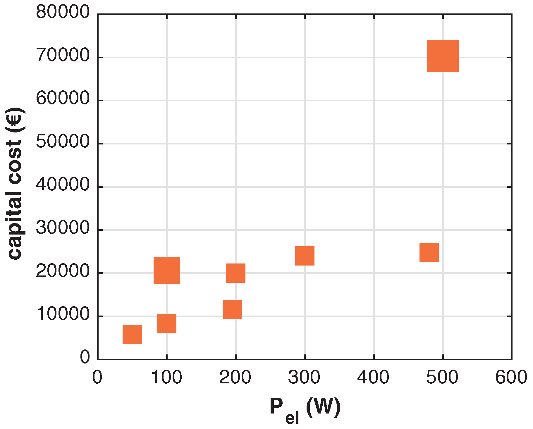
The ex-works capital cost (CAPEX) of TEGs as a function of the nominal electric power is collected in Figure 12. Note that the costs of power electronics parts (e.g., inverter) are not included in the reported amounts. If the bigger size markers are disregarded (see later), the costs range from almost EUR 6000 for the smallest power device (50 W) up to EUR 25,000 for the bigger one (500 W). The CAPEX–power relationship is linear

$${CAPEX}_{\mathrm{TEGs}}=44P_{\mathrm{el}}+3525,R^2=0.998$$

and the specific cost per unit of power considerably decreases with the TEG size: from 12,000 EUR/100 W down to 5000 EUR/100 W for 50 and 480 W power levels, respectively.

Markers of the bigger size in Figure 12 identify TEGs models suited to operate in potentially explosive atmospheres, as in the vicinity of well pads. These models are IECEx, ATEX, ETL (US) (Class 1, Zone 1) and ETL (Canada) (Class 1, Div 1) hazardous area rated. Their cost is approximately three times that of conventional models of equal power: for instance, for a 100 W TEG, the cost increases from around EUR 8000 to more than EUR 20,000 and for a 500 W, from EUR 25,000 to more than EUR 70,000.

Automatic spark ignition, safety shutoff and remote monitoring via SCADA network reduce the need for on-site interventions. Thanks to the solid state design, the recommended maintenance is one-to-two hours per year and costs roughly a few hundred euros (less than one percent of the capital cost per year). Ordinary maintenance activities aim at checking the power output and ensure a clean fuel supply by cleaning and/or changing the orifice and fuel filter. The TEGs parts most subject to wear (and which are to be replaced every few years) are electrode, ignition battery and, less frequently, burner screen. All the above operations can be made directly on field.

3.2. Fuel Cells (FCs)

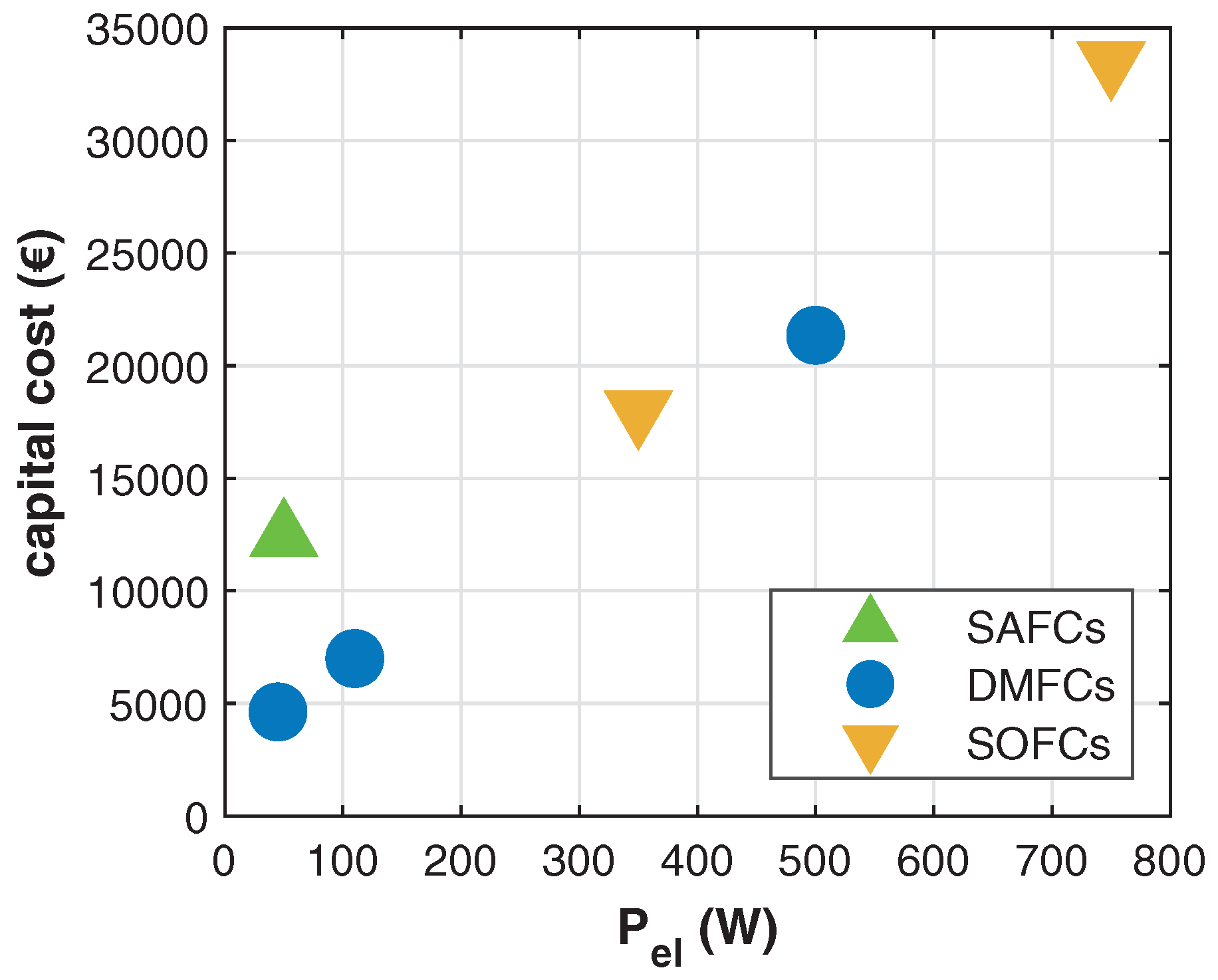
The capital cost of different types of FCs as a function of the nominal power are shown in Figure 13. Like TEGs, these costs generally do not include the inverter and remote telecommunication equipment. In the considered power range 50–800 W, capital costs span the interval EUR 5000–35,000 with differences depending on the FC type. In particular, DMFCs cost varies linearly with the power between EUR 5000 (45 W) and 20,000 (500 W). The 50 W SAFC cost (EUR 12,400) is more than twice that of an equal power DMFC. However, it has to be pointed out that this cost includes also a solar panel coupled with a controller to charge the external batteries and a modem for remote communication and operation. SOFCs cost fits the interval EUR 18,000–34,000 for the considered power range.

DMFCs and SOFCs share almost the same linear CAPEX–power relationship

$${CAPEX}_{\mathrm{DMFCs}/\mathrm{SOFCs}}=40P_{\mathrm{el}}+2745,R^2=0.993$$

whereas the specific cost per unit of power is approximately constant for SOFCs (4800 EUR/100 W), it significantly decreases with size for DMFCs (from 10,000 down to 4250 EUR/100 W for 45 and 500 W models, respectively) and it is equal to 25,000 EUR/100 W for the SAFC.

Similar to the discussion on FCs lifetime (see Section 2.2), well-defined data on maintenance costs are not available. Nevertheless, SOFCs manufacturers state that a proactive maintenance is required up to 10,000 operational hours to replace the desufurization cartridge and gas pumps, whose cost is around EUR 1000. FCs require skilled technicians, and field repairs are often unfeasible. In addition, it has to be borne in mind that the FCs capital cost sometimes includes a share to cover scheduled maintenance works.

3.3. Comparative Economic Analysis of the Different Technologies

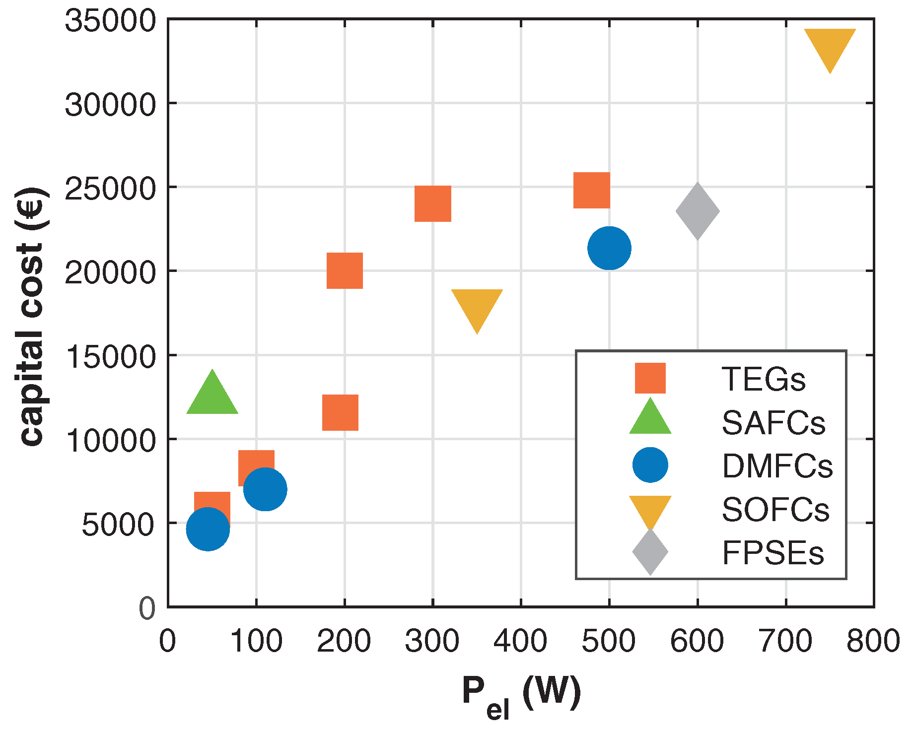
Figure 14 collects in a single plot the capital cost of TEGs (models suited to operate in potentially explosive atmospheres are not included here), FCs and FPSEs. As for FPSEs, the CAPEX of the 600 W model is EUR 24,000 ex-works, and the ordinary maintenance cost is around a hundred euros per year. Apart from the SAFC, which is more expensive, slight differences are observed among the different technologies of similar nominal power. The CAPEX–power scattered data in Figure 14 can be roughly approximated by the linear relationship

$$CAPEX=34.8P_{\mathrm{el}}+6553,R^2=0.823$$

MTs capital cost is approximately EUR 8000–12,000, depending on size and whether or not the power conditioning electronics is included.

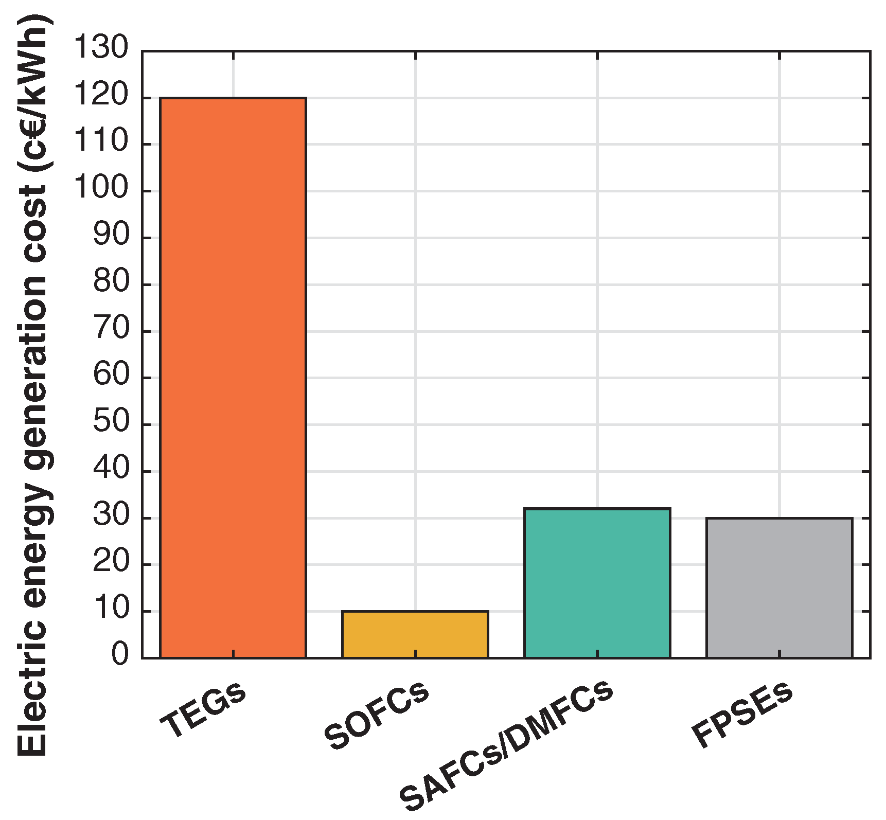
The expenditure for fuel consumption depends on both the fuel price and the conversion efficiency of the device. Accordingly, the absolute values in the following analysis are affected by price variations and, especially in the last months, volatility in the commodity markets. It is assumed that a natural gas price equal to 3 cEUR/kWh (average EU-27 natural gas price for non-household consumers in the first half 2021, [31]) and a methanol price equal to 0.32 EUR/l ([32], valid from October to December 2021). The average conversion efficiencies are 2.5%, 30%, 24% and 10% for TEGs, SOFCs, SAFCs/DMFCs and FPSEs, respectively. Based on the previous hypotheses, the outcomes in Figure 15 are found.

TEGs have definitely the highest operation cost (120 cEUR/kWh), followed with almost equal values by methanol fueled FCs (31 cEUR/kWh) and FPSEs (30 cEUR/kWh), whereas SOFCs are the cheapest ones (10 cEUR/kWh). Apparently, the relative generation costs of natural gas-fueled technologies depend only on the conversion efficiencies and the ratios of SOFCs–FPSEs–TEGs generation costs are 1:3:12.

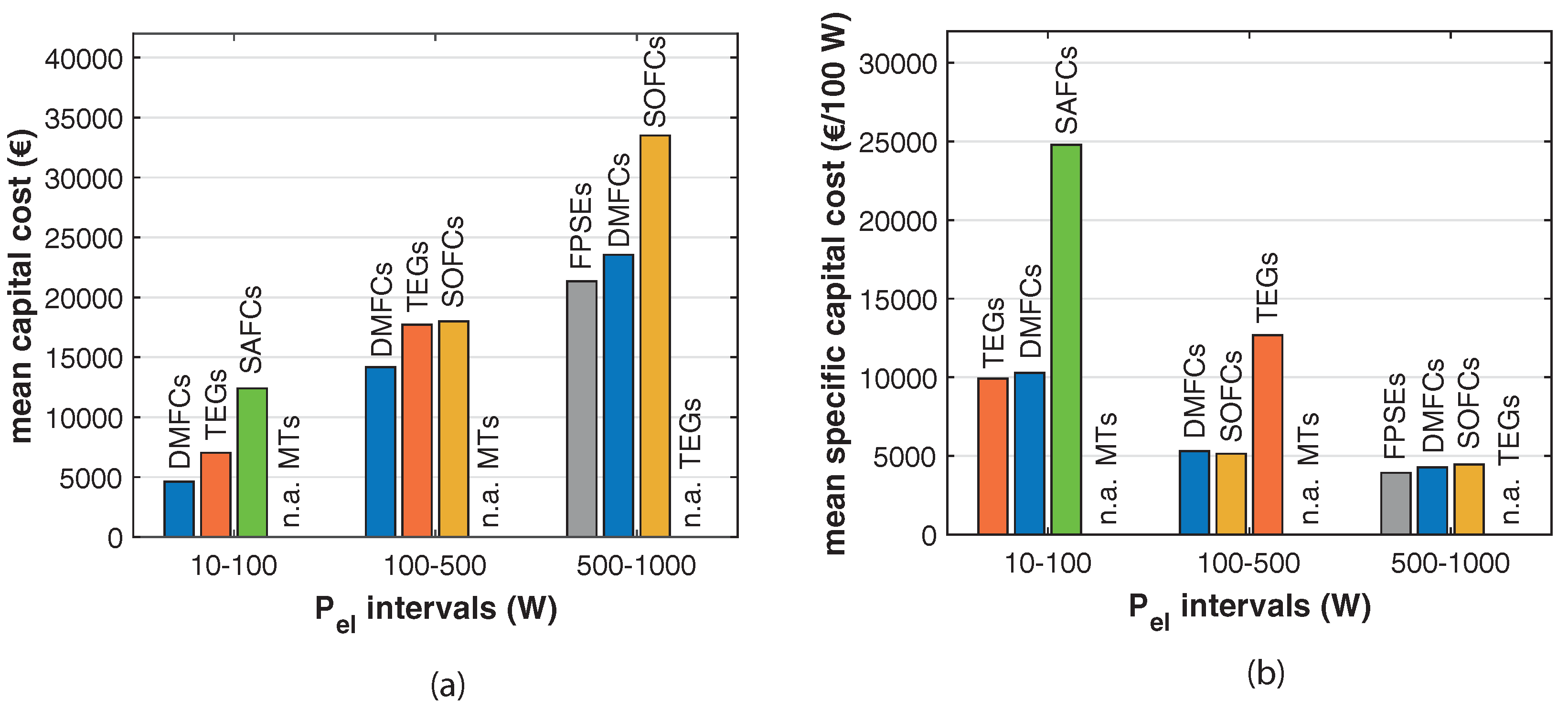
The infographics in Figure 16 show the viable technologies in three power classes (10–100, 100–500 and 500–1000 W) sorted by the corresponding mean capital cost (Figure 16a) and mean specific capital cost (Figure 16b). As for the mean capital cost, in the lower class 10–100 W, the competing options in ascending order of CAPEX are DMFCs (4625 €) < TEGs (7025 EUR) < SAFCs (12,400 EUR) and MTs. In the intermediate class 100–500 W, it results DMFCs (14,175 EUR) < TEGs (17,725 EUR) < SOFCs (18,000 EUR) and MTs. In the upper class, 500–1000 W, the order is FPSEs (21,350 EUR) < DMFCs (23,550 EUR) < SOFCs (33,500 EUR) and TEGs.

As for the mean specific capital cost, in the lower class TEGs and DMFCs are almost equal (10,000 EUR/100 W), whereas SAFCs are more expensive (24,800 EUR/100 W). In the intermediate class, the specific capital cost of DMFCs and SOFCs is almost the same (5250 EUR/100 W) and that of TEGs is slightly higher (12,700 EUR/100 W). Finally, in the upper class, the mean specific capital costs are very similar (12,700 EUR/100 W on average).

Table 3. Economic features of TEGs, SOFCs, SAFCs, DMFCs, FPSEs and MTs.

	TEGs	SOFCs	SAFCs	DMFCs	FPSEs	MTs
capital cost (€)	5750–25,000	18,000–34,000	12,500	4600–21,300	24,000	8000–12,000
specific capital cost (€/100 W)	5000–12,000	4500–5200	25,000	4250–10,000	4000	7500
maintenance cost (€/yr)	≈100	≈1000	n.a.	n.a.	≈100	n.a.
fuel consumption cost (c€/kWh)	120	10	31	31	30	N.A.

Note: N.A.: not applicable; n.a.: not available; natural gas price = 3 cEUR/kWh and methanol price = 0.32 €/L.

collects the main economic data of the technologies for remote power generation in the gas grid.

4. Environmental Impact Analysis

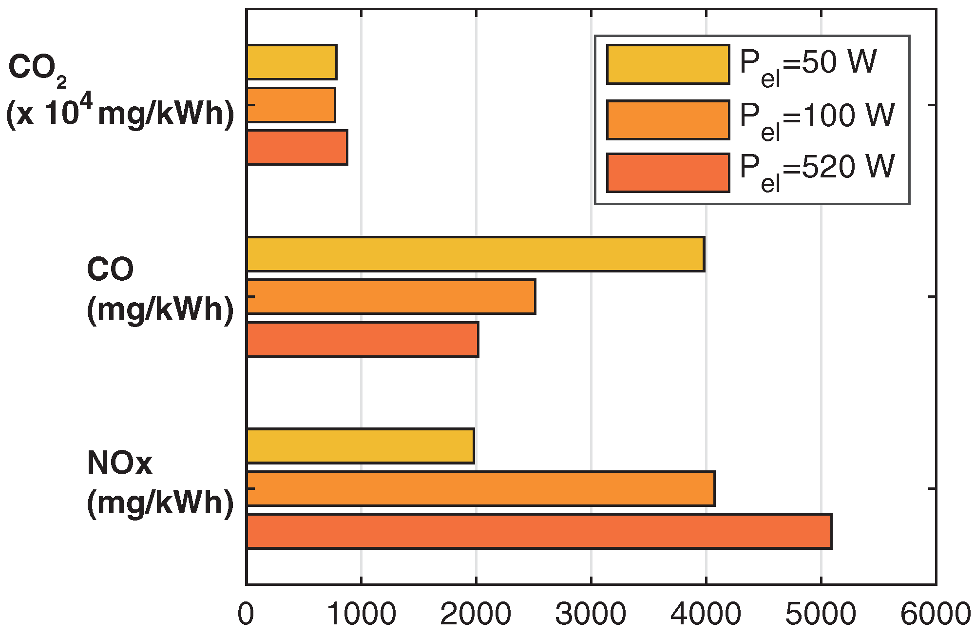
This section deals with exhausts and noise emissions from the considered technologies. All the presented data were measured by the different manufacturers and are here rearranged in a consistent form. Figure 17 shows the emissions per unit of electric energy (mg/kWh) of three TEGs (50, 100 and 520 W) at nominal conditions. Since the TEGs efficiency is comparatively low, specific emissions in the exhausts are very high. In particular, CO₂ emission is on average 8 kg/kWh, regardless of the size. The higher the TEG size, the lower the CO, which decreases from 4000 to 2000 mg/kWh for the 50 and 520 W models, respectively. An opposite trend is found for the NOx: they more than double (from 2000 to 5000 mg/kWh) when the size is increased. In brief, the emission footprint of TEGs is particularly heavy and represents a serious drawback of the low conversion efficiency.

FCs are the cleanest alternative because of the direct conversion of chemical energy into electricity (see Appendix A.2). They do not produce particles nor CO, and also NOx emission are very low (<40 mg/kWh). The average carbon footprint is 0.80 kg/kWh, which corresponds to a half of the gensets one. Noise levels during operation are less than 60 and 50 db(A) for methanol-fueled FCs and SOFCs, respectively. Accordingly, FCs are suitable for pollution and noise sensitive environments.

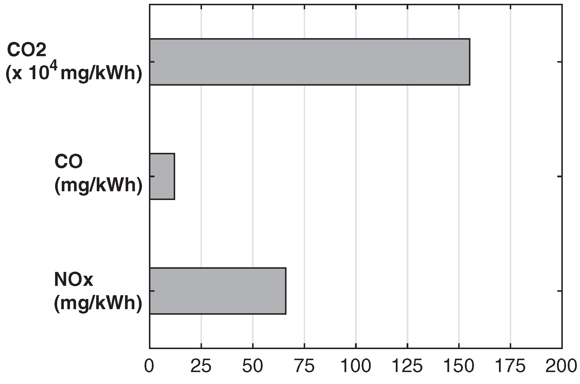
The emissions of a 5650 W FPSE are shown in Figure 18. The CO₂ emissions are comparable to those of conventional gensets of equal power and are around 1.6 kg/kWh; this value turns up to 2 kg/kWh for the 600 W model. CO emissions are 12 mg/kWh, whereas NOx almost reaches 70 mg/kWh. Noise levels are below 75 db(A).

A clear order of the exhaust impact is identified: TEGs $>>$ FPSEs > FCs > MTs. The average relative proportions of emissions from FCs-FPSEs-TEGs are 1:2.5:10 for CO₂, 1:2:100 for NOx and NA:1:200 for CO. So, TEGs emissions are one to two orders of magnitude higher than the competing technologies. As regards noise levels, the differences are limited to tens of db(A), and the resulting order is FPSEs > FCs > TEGs.

Table 4. Environmental features of TEGs, SOFCs, SAFCs, DMFCs, FPSEs and MTs.

	TEGs	SOFCs	SAFCs	DMFCs	FPSEs	MTs
CO2 (kg/kWh)	8	0.8	n.a.	n.a	1.6–2	N.A.
CO (mg/kWh)	2000–4000	N.A.	N.A.	N.A.	12	N.A.
NOx (mg/kWh)	2000–5000	<40	n.a.	n.a.	70	N.A.
noise (dB(A))	N.A.	50	60	60	75	n.a.

Note: N.A.: not applicable; n.a.: not available.

collects the main environmental data of the technologies for remote power generation in the gas grid.

5. Conclusions

The paper presents a critical comparative market review of techno-energetic, economic and environmental performances of the market available technologies for remote power generation in the range 20–1000 W for gas grid applications. The analysis makes use of several metrics and takes into account the specific technological characteristics and limitations of each technology within a consistent comparative framework. The data collected in this interdisciplinary work constitute a unique database to obtain a novel comprehensive picture of actual applications performance.

The review clearly shows that generating power in remote areas with unattended devices that must supply the requested performance with high reliability is not an easy task, and normally implies high costs and limited performance. However, it also identifies unequivocally which of the available devices should be preferred in terms of concurrent techno-energetic limitations/performance (level of power requested, acceptable level of efficiency and efficiency derate with time, and maintenance), economic and environmental performance.

In particular, TEGs cover the widest electric power interval (20–600 W) and fulfill the very low power demands. TEGs have definitely the lowest conversion efficiencies (2–3%), but they are the most reliable (and diffused) option in the gas sector, given the low relative efficiency derate with time (0.1%) and robustness resulting from their static nature (lifetime 20 yr). On the other hand, the average emissions per unit of electric energy are the highest (CO₂: 8 kg/kWh), so their usage could be hindered by the recent decarbonization policies.

In this respect, FCs are a better option (efficiencies in the range 20–30% and CO₂: 0.8 kg/kWh) but in spite of the advancements during the last decades, their technological maturity is still low. In fact, FCs relative efficiency derate with time is very high (10%, 22%, 87% for SOFCs, SAFCs and DMFCs, respectively), making lifetimes are rather short (1000–10,000 h). In addition, their operation in harsh environmental conditions poses some risks on their reliability, they suffer fuel impurities, and field repairs are often unfeasible. SOFCs cover the upper half of FC power domain (350–900 W), whereas DMFCs and SAFCs generally meet power demand less than 100 W.

FPSEs are a promising and still less known technology for the gas grid applications of relatively high power (600 W). Despite the low number of installations worldwide and the resulting scarcity of data, it can be stated that FPSEs are halfway between TEGs and FCs in terms of techno-energetic metrics: efficiency around 10%, low relative efficiency derate with time, considerable lifetimes (10 yr) and emissions comparable to those of internal combustion engines (CO₂: 2 kg/kWh).

MTs deserve a separate mention because they are small and robust energy harvesting devices (10–150 W, lifetime 7 yr) with a neutral environmental impact. However, MTs producibility depends on the variable pressure drop imposed by the gas network, and therefore, their reliability could be compromised by external factors.

In terms of power intervals, three power thresholds are broadly identified: below 50 W, TEGs or MTs are necessarily chosen; between 50 and 600 W, TEGs and FCs are both viable options; and over 600 W, SOFCs or FPSEs are preferred.

The economic analysis reveals reveals light differences among the technologies of similar nominal power, and a linear regression of all CAPEX–power data fits quite well. In contrast, the expenditure for fuel consumption is very different, depending on the conversion efficiency and fuel cost. TEGs have definitely the highest operation cost (120 cEUR/kWh), followed with almost equal values by methanol fueled FCs (31 cEUR/kWh) and FPSEs (30 cEUR/kWh), while SOFCs are the cheapest ones (10 cEUR/kWh).

Table 5. Main advantages and disadvantages of the power generating technologies.

	Advantages	Disadvantages
TEGs	wide power interval	very low efficiency
	very low efficiency derate	high emissions
	very long lifetime	high operation cost
	many installations
	ATEX certified
FCs	high efficiency	very high efficiency decay
	low emissions	short lifetime
	low operation cost
FPSEs	high efficiency	only for “high” power
	low efficiency derate	few installations
	long lifetime
MTs	robustness	depend on grid boundary conditions
	no emissions
	long lifetime
	ATEX certified

summarizes the main advantages and disadvantages of each technology.

The authors’ expectation is that the critical indications extracted from this review, first in the literature, may constitute helpful guidelines for grid operators that have to knowingly choose power generator systems for remote applications.