Article

Multi-Step Short-Term Wind Speed Prediction Models Based on Adaptive Robust Decomposition Coupled with Deep Gated Recurrent Unit

1
School of Science, Shanghai Institute of Technology, Shanghai 201418, China
2
Shanghai Key Laboratory of Mechanics in Energy Engineering, Shanghai Institute of Applied Mathematics and Mechanics, School of Mechanics and Engineering Science, Shanghai Frontiers Science Base for Mechanoinfomatics, Shanghai University, Shanghai 200072, China
3
Guangdong Provincial Key Laboratory of Turbulence Research and Applications, Southern University of Science and Technology, Shenzhen 518055, China
4
School of Urban Construction and Safety Engineering, Shanghai Institute of Technology, Shanghai 201418, China
5
School of Mechanical Engineering, Shanghai Institute of Technology, Shanghai 201418, China
*
Author to whom correspondence should be addressed.
Energies 2022, 15(12), 4221; https://doi.org/10.3390/en15124221
Submission received: 20 April 2022 / Revised: 30 May 2022 / Accepted: 4 June 2022 / Published: 8 June 2022

Abstract

:
Accurate wind speed prediction is a premise that guarantees the reliable operation of the power grid. This study presents a combined prediction model that integrates data preprocessing, cascade optimization, and deep learning prediction to improve prediction performance. In data preprocessing, the wavelet soft threshold denoising (WSTD) is employed to filter the blurring noise of the original data. Then, the robust empirical mode decomposition (REMD) and adaptive variational mode decomposition (AVMD) are adopted to carry out a two-stage adaptive decomposition. Spearman correlation is used to quantify the mode that need to be decomposed for the second time. In the cascade optimization, the hybrid grey wolf algorithm (HGWO) is employed to optimize the parameters of the VMD and the gated recurrent unit (GRU), which overcomes the problem of empirical parameter adjustment. The HGWO is also adopted in the prediction strategy to optimize the GRU model to predict the grouped intrinsic mode functions (IMFs). Lastly, the final wind speed prediction result is obtained by superimposing the values of all the predicted models. The proposed model was validated with the measured wind speed data of the four quarters in the Bay area of China and was compared with 20 models of the classic method to further evaluate the effectiveness of the model. The results show that the whole process of the proposed model is adaptive, the final multi-step prediction performance is good, and high prediction accuracy can be attained.

1. Introduction

Wind energy is a highly efficient and renewable energy. Its development and utilization have been widely recognized [1]. The intermittent and randomness of wind speed bring stern challenges for the stable operation of power systems [2,3]. Accurate prediction of wind speed will benefit the exploitation of wind energy. Wind speed prediction is a hot research topic, and a number of prediction methods have been proposed over the past decades which can be classified into physical models, statistical models, machine learning models, and combination models [4].
As wind is a multi-scale physical phenomenon, numerical weather predictions (NWP) provide straightforwad wind speed predictions with physical advantages [5]. The physical model based on NWP applies historical meteorological factors such as temperature and barometric pressure to predict the wind speed over a long period [6]. Additionally, wind speed prediction is applied using physical approximation and spatial correlation fluid dynamics models [7,8]. However, the physical model is complex in modeling, poor in prediction accuracy, and its scope of application is limited. It is not suitable for short-term wind speed prediction. Recently, a data-driven method based on stacked bidirectional long short-term memory (BiLSTM) for wind turbine wake prediction was proposed by Geibel and Bangga [9], and satisfactory prediction accuracy was achieved, indicating that a data-driven approach can offer an alternative to conventional prediction methods.
Statistical models use the linear mapping relationship between historical weather conditions and wind speed and utilize series data to predict the future wind speed series through this relationship [10]. Traditional statistical modes such as auto-regression (AR) [11], auto-regressive moving average (ARMA) [12], auto-regressive integrated moving average (ARIMA), and auto-regressive conditional heteroskedasticity (ARCH) are widely used in the field of time series prediction [13]. For instance, the ARCH model was used to predict the revenues of the financial stock market [14]. Radziukynas adopted a classical ARIMA model to predict short-term wind speed series [15]. Tian and Wang et al. proposed a prediction method based on ARMA and echo state network (ESN) compensation to deal with the statistical characteristics of wind speed series, which can obtain accurate prediction results [16]. As mentioned above, the statistical models often uses the historical wind speed data to establish linear wind speed prediction models, but due to the strong nonlinearity of data, the model parameters are difficult to determine, and the prediction accuracy is not satisfied.
To improve the accuracy of the wind speed prediction, statistical models based on artificial intelligence were proposed. Compared with statistical models, artificial intelligence prediction models have outstanding capabilities in processing nonlinear wind speed time series. With the rapid development of artificial intelligence, great effort has been made to improve the accuracy and universality of wind speed prediction. Nair and Jisma presented ANN and ARIMA to predict the wind speed at three different locations in India in different time periods, which reduces the nonlinear characteristics of the wind speed series [17]. In another work, Shukur and Lee proposed the Kalman filter (KF) and an ANN hybrid model based on ARIMA to deal with the nonlinearity and uncertainty of wind speed [18]. Machine learning models based on neural network have became popular in short-term wind speed prediction [19]. For example, the prediction models based on back-propagation neural networks (BPNN) [20], least square support vector machines (LSSVM) [21], support vector regressions (SVR) [22], extreme learning machines (ELM) [23], Elman neural networks (ENN) [24], adaptive wavelet neural networks (AWNN) [25], and recurrent neural networks (RNN) [26] perform well when dealing with time series with nonlinear characteristics. However, these techniques are all built with single neural network models, which may result in local optimization or over-fitting problems in short-term wind speed prediction.
To improve the prediction performance, researchers introduced combination models to integrate the advantages of every single model. The combination prediction model combines data preprocessing, an optimization algorithm, a and predictor, which shows outstanding performance in wind speed prediction. The data preprocessing strategy composed of outlier detection and data decomposition can greatly ameliorate the prediction performance of the whole model [27]. The missing original data and outlier problems caused by human, weather, and other factors are the primary problems to be addressed in the field of wind speed prediction. After outlier processing, taking into account the nonlinearity and noise characteristics of wind speed [28], the data decomposition method can drop the instability of wind speed correlation series and abandon redundant information and combine with a machine learning model to enhance the predictability of wind speed [29]. For instance, Mi and Zhao [30] applied the singular spectrum analysis (SSA) model to denoise the original wind speed data to capture the complex dynamic characteristics of wind speed, which combines the adaptive structure learning of neural networks with long- and short-term memory networks (LSTM) to predict wind speed in three wind farms in Xinjiang, China. The proposed model has good prediction performance. A hybrid method of empirical mode decomposition (EMD) and ARIMA-ANN is proposed to improve the prediction accuracy of time series [31]. Zhan and Tian et al. [32,33] studied the two-stage decomposition model of the complementary ensemble empirical mode decomposition (CEEMD) and local mean decomposition (LMD) to achieve intrinsic mode functions (IMFs) of different regularity degrees, which was applied to (support vector machine) SVM and T-S fuzzy neural network (FNN) prediction. Duan et al. [34] proposed variational mode decomposition (VMD) to extract the local characteristics of the original wind speed series and constructed an integrated prediction model using deep belief network (DBN) optimized by particle swarm optimization (PSO), which overcomes the shortcomings of linear weighted combination, and the performance of the prediction model is better than many traditional models. Meanwhile, the wavelet transform (WT) [35] method shows advantages in extracting and studying the characteristics of wind speed in the time domain and frequency domains and solves the randomness and complexity of wind speed signals. Liu et al. [36] designed a hybrid model combining wavelet decomposition (WD) and LSTM to predict China’s wind power generation in the next two years. The experiment showed that this model effectively improves the accuracy of the prediction.
In addition to the above models, the decomposition-based method may contribute to large differences in prediction performance. For the decomposed models, in terms of generalization performance, sometimes they cannot capture the characteristics of wind speed. As such, the prediction accuracy and training speed of the model are affected because the advantage of parameter optimization is not considered. To avoid these problems, an adaptive short-term wind speed predictor is formed based on the model of optimization algorithm [37], which reduces the prediction error and achieves good prediction results. As an example, Bai et al. [38] proposed a dynamic integrated wind speed prediction model, a hybrid model composed of VMD and a genetic algorithm (GA)-optimized double-layer staged training echo state network (DESN), which used the DESN to process nonlinear series and capture time information of different time scales, and the model has better time-varying and robustness through nonlinear weighted combination mechanism. Wu and Wang et al. [39], considering the accuracy and stability of the model, applied multi-objective grey wolf optimization (MOGWO) to optimize ELM to form a new integrated global wind speed prediction method. Neshat [40] combined effective hierarchical decomposition technology and deep learning optimization methods to develop a combined model with deep feature selection and optimal intrinsic mode functions to predict the forward time step of wind speed data from Baltic offshore wind farms. Tian et al. [41] utilized EMD to decompose the original wind speed data into IMFs with different frequencies, and then embedded multiple IMFs into the enhanced network of improved sparrow search algorithm (ISSA) optimized LSTM for prediction, which solved the problem of slow convergence speed of previous models and being easy to fall into local optimum. The results indicate that the model of EMD and ISSA optimization LSTM has good predictive ability. The literature review shows that using the diversity of optimization algorithms to predict the wind speed prediction model with the best parameters, which can improve the prediction accuracy and stability of the model to a certain extent.
Short-term prediction is to predict wind speed from 10 min to 30 min in advance. It is conducive to the timely and reasonable dispatching of the power grid, maintenance of power quality, and the stable operation of the power system. Because of the uncertainty of wind speed, short-term wind speed prediction has great practical significance and application value. In the field of short-term wind speed prediction, wind speed is an important indicator that affects wind power generation. However, due to many uncertain factors, the integrity of the original wind speed data has been destroyed. The rapid change in wind speed leads to the nonlinear and nonstationary characteristics of wind speed series. EMD is an adaptive data decomposition method [42] suitable for processing nonlinear and unstable time series, but its decomposition has the problem of model-mixing and the uncertainty of the maximum number of iterations in the sifting process, which affects the performance of the wind speed data decomposition method. Hence, VMD has a better decomposition effect and is more robust when dealing with complex wind speed time series [43]. What is undesirable is that VMD requires artificial parameters and lacks rigor. Therefore, in consideration of the completeness and predictability of wind speed data, data preprocessing strategy plays an important role in the study of short-term wind speed prediction.
Reviewing the above-mentioned methods, the combined method based on the decomposition denoising method and the optimization parameter method are discussed, and the research contributions of these methods and their shortcomings are summarized. To this end, this study considers the generalization ability and stability of the prediction model and develops a short-term multi-step wind speed prediction method with adaptive robust decomposition characteristics that combines a data-processing strategy, a cascade optimization strategy, and a prediction strategy [44]. The method includes a data preprocessing strategy based on wavelet soft threshold denoising (WSTD), robust empirical mode decomposition (REMD) and variational mode decomposition (VMD), cascade optimization based on the hybrid grey wolf optimization algorithm (HGWO) strategy, and a prediction strategy based on deep gated recurrent unit (DGRU), which is achieved satisfactory results in the field of short-term wind speed prediction. The primary innovations and contributions of this research are as follows:
(1)
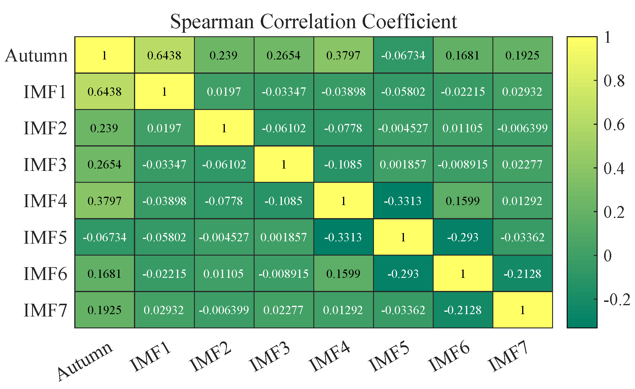
Data preprocessing strategy: A novel and efficient two-stage data preprocessing technology is proposed. WSTD filters out the redundant noise of the original wind speed series. One-stage REMD decomposes to obtain a series of IMFs to eliminate random fluctuations. To reduce the error, Spearman correlation analysis is used to analyze the correlation between each IMF and the original wind speed time series, group reconstruction, reduce the accumulation of errors, and prepare high-quality data for prediction purposes.
(2)
Cascade optimization strategy: The cascading optimization strategy based on HGWO, which is used for the first time, and the optimized VMD is used to decompose the IMFs with strong correlation in the wind speed correlation series in the second stage to further explore the potential characteristic information of the wind speed. On this basis, it is more robust to deal with time series of complex characteristics.
(3)
Prediction strategy: The strategy of cascading optimization is adopted to dynamically analyze the optimal input parameters and optimal network structure of the GRU deep learning model, and the reorganized wind speed correlation sub-series are predicted and superimposed in the future time step to complete deeper wind speed characteristic extraction and learning, which greatly enhance the stability and generalization of the model.
(4)
The combined multi-step wind speed prediction method of WSTD, REMD, and HGWO-VMD-GRU is proposed, which integrates the advantages of each single model. The wind speed datasets of different seasons in the Shanghai Bay area are selected to verify the validity of the model, and the final conclusion is reached by testing and analyzing three different benchmark models with the classic single models, the decomposition optimization models, and other combined models.
The paper is organized as follows. In Section 2, we introduce the basic theory of the relevant methods and the framework of the proposed prediction system. Section 3 gives a comprehensive discussion on the experimental results from various prediction models. In Section 4, we draw the conclusion.

2. Related Methodology

An adaptive decomposition integrated combined wind speed prediction system has been developed in this study. The basic framework of the proposed model is shown in Figure 1. First, a wind speed data preprocessing strategy based on WSTD and REMD is proposed. Meanwhile, the Spearman correlation coefficient is used to quantitatively analyze the wind speed component after pretreatment to reduce the accumulation of errors. Secondly, the cascade optimization strategy of VMD and GRU is optimized based on HGWO. Finally, the prediction strategy based on GRU is proposed. It can be observed that each integrated model has adaptive characteristics, which makes the whole prediction system more robust and accurate. The strategies adopted for data preprocessing, cascade optimization and building prediction modeling are introduced in detail in the following.

2.1. Data Preprocessing

2.1.1. Data Collection

The wind speed series used in this study are measured from the Shanghai Bay area in China in 2019 and were provided by Fengxian Meteorological Bureau. Four different short-term wind speed samples in the four seasons are selected as datasets. The four datasets are termed as dataset A, B, C, and D. The data sampling interval is 10 min, and there are 2000 data in each dataset, as shown in Figure 2. The average, standard deviation, median, variance, and box plot are shown in the figure as well. The difference among the four datasets are reflected from the statistics.

2.1.2. Data Denoising Based on WSTD

WSTD is a time-frequency domain signal processing method based on wavelet transform (WT) [45]. WT is usually used for denoising or filtering of strongly nonstationary signals. There are a variety of criteria for selecting wavelet bases and thresholds in WT, and an inappropriate selection will disrupt the performance. Suppose the measured noisy wind speed data are f ( t ) . They can be decomposed as:
f ( t ) = x ( t ) + δ e ( t ) ,
where t is the time interval, x ( t ) is the real wind signal, e ( t ) is the Gaussian white noise, δ represents the correlation coefficient of the noise.
WSTD generally includes three steps, i.e., WT, threshold function, and wavelet reconstruction. In WT, the denoising effect is quantified by the signal-to-noise ratio (SNR) and the RMSE. The larger the SNR or the smaller the RMSE is, the better the noise reduction. The denoising effect of WT was tested on dataset C. Table 1 demonstrates the SNR and RMSE obtained with different wavelet basis functions. The results suggest that WT with db4 wavelet basis function shows the best noise reduction.
Threshold function is used to quantify the high-frequency coefficients at different scales obtained by WT. The selection of the threshold function has a great influence on the denoising results. The two well-known threshold functions are the hard threshold function and the soft threshold function. The hard threshold function is not continuous, which leads to additional oscillations in the signal reconstruction. On the contrary, the soft threshold function maintains good continuity by flexibly managing the discontinuity of the hard threshold in various threshold estimation methods and enhances the effect of denoising in the wind speed prediction models. The soft threshold function is:
W X ^ = s i g n ( W X ) | W X | , | W X |   λ 0 , | W X |   < λ
where W X is the WT coefficient, W X ^ is the calculated WT coefficient, λ indicates the threshold, s i g n denotes the symbolic function.
Finally, the denoised wind speed time series is obtained by wavelet reconstruction, which reconstructs the processed high- and low-frequency wavelet coefficients.
Overall, the denoising effect of WSTD is better than the traditional denoising methods. The denoised datasets by WSTD are shown in Figure 3, and it is observed that the wind speed time series are smoother than the original ones.

2.1.3. One-Stage Decomposition Based on REMD

The nonlinearity and nonstationarity of wind speed seriously affect its forecast accuracy. The proper decomposition of the original wind speed data can effectively alleviate the complex characteristics of the wind speed and improve the prediction accuracy. The usually used decomposition methods such as EMD and EEMD require manually preset thresholds, which are not adaptive, resulting in mode-mixing problems after decomposition and affecting the prediction results.
The implementation of EMD is mainly based on three parameters: envelope estimation, boundary condition and sifting stop criterion (SSC). The classical cubic spline interpolation method and mirror extension method are adopted for envelope estimation and boundary condition. Among them, the SSC parameter has the greatest impact on the accuracy and efficiency of EMD. This parameter directly affects the sifting iterations number and then controls the decomposition component of EMD, but it opts to cause the ‘under-sifting’ or ‘over-sifting’ phenomenon. Therefore, the study of SSC is essential to deal with the mode-mixing problem in EMD. The definition of SSC parameter is as follows: (1) the number of extreme points and zeros must be equal or no more than one, i.e., N z o r e s N e x t r e m e 1 ; (2) if the envelope mean signal m i k [ n ] of EMD is 0, the sifting process stops, that is, lim k m i k [ n ] = 0 . The objective function is designed to describe the envelope mean signal, and the RMS and EK are taken into account, so that all sample points of the signal uniformly tend to zero. Based on this, Liu et al. [46] exploited SSC for adaptive control of the sifting process, which is used to ease the mode-mixing phenomenon and improve the decomposition results, so as to improve the accuracy of wind speed prediction. The improved EMD performs robust decomposition of wind speed data owing to its adaptability. The original wind speed series is written as:
x ( t ) = k = 1 i I M F K ( t ) + r i ( t )
The detailed processes of robust empirical mode decomposition (REMD) are as follows:
Step 1:
Initialize parameters k and i, set the maximum number of sifting iterations I m a x ;
Step 2:
Find the maximum and minimum values of the wind speed signal h i k 1 [ n ] . The upper and lower envelopes are obtained by cubic spline interpolation. Then, calculate the average value of the upper and lower envelopes m i k [ n ] :
h i k [ n ] = h i k 1 [ n ] m i k [ n ]
where h i k [ n ] indicates the signal after the ith IMF sifting k times;
Step 3:
Apply the objective function of SSC to calculate the objective value f i k . The objective function is defined as follows:
f i k = R M S ( m i k [ n ] ) + | E K ( m i k [ n ] ) |
R M S i k = 1 N s n = 1 N s ( m i k [ n ] ) 2
E K i k = 1 N s n = 1 N s ( m i k [ n ] m ¯ ) 4 [ 1 N s n = 1 N s ( m i k [ n ] m ¯ ) 2 ] 2 3
where m ¯ stands for the arithmetic mean of m i k [ n ] ;
Step 4:
Execute SSC to determine the sifting stop process. If it is satisfied at the same time, stop and output; otherwise, return to step 2 and continue to iterate until the maximum number of sifting iterations I m a x is received, and output the k-2nd h i k 2 [ n ] as I M F i . The two criteria are expressed as follows:
f i k 2 < f i k 1 , f i k 1 < f i k a b s ( N z o r e s N e x t r e m e ) 1

2.2. Cascade Optimization

2.2.1. The Hybridizing Grey Wolf Optimization Algorithm

The HGWO uses the differential evolution (DE) to carry out population mutation in order to maintain the diversity of the population and then takes it as the initial population of the GWO to find the optimal individual [47]. The crossover and selection operation of DE are used to update the positions of other grey wolf individuals, and the cycle process is used to obtain the optimal solution. Step 4 in Figure 1 shows the flow chart of hybrid grey wolf algorithm. The process of DE and GWO are presented below.
DE is a random selection model that simulates biological evolution, which is used to solve global optimization problems. The implementation of DE includes initialize population, mutation, crossover, and selection operations as explained below.
Initialize population: Randomly generate population individuals.
Mutation: The operation of the mutated individual is implemented as follows:
h i j t + 1 = X p 1 t + F ( X p 2 t X p 3 t )
where F is the scaling factor; t is the current iteration number; p 1 , p 2 , and p 3 are a random unequal integers in N that are not equal to t; and N is the population size.
Crossover: Crossover operation can increase the diversity of the population, the operation is applied as below:
U i j t + 1 = h i j t + 1 , r a n d ( j ) C R o r j = r a n d ( 1 , n ) X i j t , r a n d ( j ) > C R o r j r a n d ( 1 , n )
where C R represents the crossover probability between 0 and 1, j is a random integer between 1 and D, and D is the dimension of the solution.
Selection: Utilize a greedy strategy to select the offspring of an individual, as defined below:
X i t + 1 = U i t + 1 , f ( U i t + 1 ) < f ( X i t ) X i t , f ( U i t + 1 ) f ( X i t )
where X i t + 1 is the ith current population individual in the t+1 generation population, and U i t + 1 is the ith crossover individual in the t+1 generation population.
According to the DE algrithm, the superiority of the progeny population can be guaranteed, and the average performance of the population can be improved.
GWO is an intelligent optimization algorithm inspired by the predation behavior of grey wolves in nature. With its advantages of simple mechanism, strong global search ability, and few adjustable parameters, it achieves parameter optimization based on the mechanism of wolf group cooperation. Wolves have a very strict social hierarchy. As shown in Figure 4, the wolf pack is divided into four levels to simulate leadership levels. The social hierarchy of grey wolves plays an important role in pack hunting. The predation process is completed under the leadership of Wolf α , Wolf β , and Wolf ζ , and the existence of Wolf ω maintains the stability of the pack hierarchy. The hunting of grey wolves includes the following three main components:
Pursuing prey: The behavior of grey wolves chasing prey is defined as follows. The distance D between the two is expressed as:
D = | C · X p ( t ) X ( t ) |
C = 2 r 1
where t denotes the current iteration, A and C are coefficient vectors, X ( t ) represents the position of the grey wolf after iteration t, X p ( t ) stands for the position of prey after iteration t, and C is the swing factor.
The grey wolves’ position update formula is described as follows:
X ( t + 1 ) = X p ( t ) A D
A = 2 a r 2 a
where r 1 and r 2 are random vectors in [0, 1], A is the convergence factor, and a decreases linearly from 2 to 0 as the number of iterations increases.
Rounding up prey: Grey wolves identify the location of their prey and encircle their prey. This behavior is depicted as follows:
D α = | C 1 X α ( t ) X ( t ) |
D β = | C 2 X β ( t ) X ( t ) |
D ζ = | C 3 X ζ ( t ) X ( t ) |
Attack prey: Prey stops moving, and the grey wolf attacks to complete the hunt:
X 1 = X α ( t ) A 1 D α
X 2 = X β ( t ) A 2 D β
X 3 = X ζ ( t ) A 3 D ζ
X p ( t + 1 ) = X 1 + X 2 + X 3 3
where X α , X β , and X ζ indicate the position vectors of α , β , and ζ wolves, respectively, and D α , D β , D ζ are the distances from the current wolf to the three optimal solutions, respectively.
To avoid the defects of local optimization and poor stability of DE and GWO, the hybrid of the two algorithms, namely, DE-GWO, improves the global search ability and shows the adaptive and fast convergence ability in wind speed prediction.

2.2.2. Two-Stage Decomposition Based on VMD

VMD is a signal decomposition method for nonlinear and nonstationary characteristics proposed by Dragomiretski et al. [48]. It has the characteristics of being adaptive, quasi-orthogonal, and completely nonrecursive, the essence of which is to construct and solve the variational problem. The VMD method is as follows:
To obtain a unilateral spectrum, the means of the Hilbert transform are adopted to calculate the associated analytic signal for each mode:
( δ ( t ) + j π t ) u k ( t )
The center frequency of each mode is assessed:
[ ( δ ( t ) + j π t ) u k ( t ) ] e j ω k t
The L2 norm of the gradient for the demodulated signal is employed to calculate the bandwidth of each mode. The variational constraint problem is constructed as follows:
min u k , ω 2 k t [ ( δ ( t ) + j π t ) · u k ( t ) ] e j ω k t 2 2
k u k ( t ) = f ( t )
where f ( t ) represents the original signal, u k is each modal component, ω k indicates the central frequency of each modal, δ ( t ) denotes the unit impulse function, and K is the total number of modal components.
Solving variational problems: Introduces the Lagrange multipliers λ and quadratic penalty factors α , so that the constructed constrained variational solution problem becomes an unconstrained variational decomposition problem. The augmented Lagrange function of the original constrained variational solution problem can be expressed as:
L ( u k , ω k , λ ) = α k = 1 K t [ ( δ ( t ) + j π t ) · u k ( t ) ] e j ω k t 2 2 + f ( t ) k = 1 K u k ( t ) 2 2 + λ ( t ) , f ( t ) k = 1 K u k ( t )
The Alternating Direction Multiplier Method (ADMM) is used to search the saddle point of the augmented Lagrange function to solve the variational problem, where each mode u k , center frequency ω k , and Lagrange operator λ are iteratively updated as follows:
u ^ k n + 1 ( ω ) = f ^ ( ω ) i < k u ^ k n + 1 ( ω ) i > k u ^ k n ( ω ) + λ ^ ( ω ) 2 1 + 2 α ( ω ω k n ) 2
ω k n = 1 = 0 ω | u ^ k n + 1 ( ω ) | 2 d ω 0 | u ^ k n + 1 ( ω ) | 2 d ω
λ ^ n + 1 ( ω ) = λ ^ n ( ω ) + τ ( ω ^ k u ^ k n + 1 ( ω ) )
where τ is the update parameter.
If the following discriminant formula is met, stop the iteration; otherwise, repeat the above operation:
k u ^ k n + 1 ( ω ) u ^ k n ( ω ) 2 2 u ^ k n ( ω ) 2 2
VMD exhibits some advantages over traditional recursive mode decomposition in signal decomposition problems, and the decomposition result is determined by the number of modal components and the secondary penalty factor. The remaining parameters have weak effect on the decomposition result and are generally set with default values. However, the choice of the two key parameters is empirical. Usually, the optimal combination of the parameters is not adopted. The adaptive decomposition of VMD optimized by HGWO overcomes this deficiency, which provides the best decomposition as well as sufficient feature mining of the data.
In this study, the decomposition performance of VMD is measured with the minimum envelope entropy (MEE). Taking the MEE as the fitness function of HGWO algorithm, under the influence of a set of modal decomposition parameters and the combination of the secondary penalty factor parameters, the one with the smallest entropy value is selected as the MEE, which is recorded as the best fitness function MEE. Therefore, the parameter combination corresponding to the global optimal component is obtained, namely, K and α . The steps to solve the M E E are as follows:
b j = a j j = 1 M b j , j = 1 , 2 , , M
I M F E E ( k ) = j = 1 M b j log 2 ( b j )
M E E = min ( I M F E E ( 1 ) , , I M F E E ( k ) )
where M is the length of the modal component of the wind speed time series by VMD, b j is the normalized envelope of the modal components, a j is the envelope amplitude of the jth point of the modal component after VMD, and I M F E E ( k ) is the envelope entropy of a modal component.
The parameter determination algorithm based on the MEE is used to find the optimal combination of VMD parameters and the fitness function set by HGWO, which solves the problem of the under-decomposition and over-decomposition of the modal caused by the improper selection of VMD parameters, and forms an adaptive wind speed decomposition method.
VMD is commonly used to perform data preprocessing in the field of wind power prediction, which can extract abundant characteristic information from wind speed signals. In this study, the local characteristics of the wind speed time series are extracted through the secondary decomposition of VMD with the purpose of tracking wind speed change information in real time.

2.3. Prediction Model

Deep Gated Recurrent Unit

GRU is a network model for processing time series. It is a variant of RNN [49], which simplifies the network structure while ensuring the original accuracy of LSTM, has strong learning ability and efficiency, and can selectively forget or retain the input historical information through the update gate and reset gate, so as to realize the prediction of future data.
The GRU model can control the degree of the state information of the previous moment by updating and resetting the gate. The GRU network structure is shown in Figure 5. The parameters that the entire model needs to be trained are W z , W r , and W h , and the forward training process is:
z t = σ ( W z h h t 1 + W z x x t )
r t = σ ( W r h h t 1 + W r x x t )
h ˜ t = t a n h ( W h h ( r t h t 1 ) + W h x x t )
h t = ( 1 z t ) h t 1 + h ˜ t z t
where W z h , W z x is the weight matrix of the updated gate, W r h , W r x is the weight matrix of the reset gate, W h h , W h x is the weight matrix when calculating the output candidate value h t , and ⨀ is the product of the elements of the matrix.
The concrete procedures of HGWO-GRU (DGRU) are described as follows:
Step 1:
Define the parameters of HGWO, such as population size N, maximum number of iterations t m a x , and crossover probability parameters C R .
Step 2:
Initialize the parameters a , A , C , implement DE mutation and competitive selection on the population individuals according to the formula, and generate the initial population.
Step 3:
Apply formula (12)–(21), calculate the objective function value of each grey wolf individual in the population, and select the positions of the three individual grey wolves X α , X β , and X ζ with the optimal value. Then, calculate the distance between other grey wolves in the population and the optimal individual position, and update the current position.
Step 4:
According to the formula (9)–(11), cross the positions of individuals and screen out new individuals.
Step 5:
Perform formula (22), calculate the target fitness value of all grey wolf individuals, and update the grey wolf individuals in the three optimal positions of X α , X β , and X ζ .
Step 6:
Cycle process, judge whether the maximum number of iterations is reached; if so, save the global optimal solution and exit. Otherwise, return to step 3 to continue the iterative update.
Step 7:
Output the optimal position, that is, X α . The GRU network determines the optimal combination parameters (GRU-size, Learning-rate).
For the construction of prediction model, the rolling prediction mechanism is used in training set and test set. Each input of 3 measured data corresponds to 1 output as the predicted value. Accordingly, 2000 data are formed into 1997 datasets, of which the first 1800 sets of data are used as training sets. The remaining 197 sets of data are used as the test set. In addition, before entering the model, the wind speed time series are normalized, and, finally, the future wind speed data are predicted by one, two, and three step ahead. The expressions of the one-step and multi-step predictions are as follows. Assuming the wind speed series is ( x 1 , x 2 , , x n ) , the length of Moving Window is h. In m-step prediction, the moving step length of the Moving Window is m. Note that the length h = 3 is adopted in our following predictions based on multiple trials.
The prediction formula at time t in one-step prediction is:
x 1 , x 2 , , x h y h + 1 , t = 1
x 2 , x 3 , , x h + 1 y h + 2 , t = 2
x 1 + k 1 , x 1 + k , , x h + k 1 y h + k , t = k
The prediction formula at time t in m-step prediction is:
x 1 , x 2 , , x h y h + 1 , , y h + m , t = 1
x 1 + m , x 2 + m , , x h + m y h + m + 1 , , y h + 2 m , t = 2
x 1 + ( k 1 ) m , x 2 + ( k 1 ) m , , x h + ( k 1 ) m y h + ( k 1 ) m + 1 , , y h + k n , t = k

3. Experimental Results and Discussion

This section introduces the Evaluation index, Denoising verification, Model parameters selection, and Experimental results.

3.1. Evaluation Index

To evaluate the performance of the prediction model, five evaluation indicators are used in this paper, which are the Mean absolute error, Root mean square error, R-squared, Theil inequality coefficient, and Square sum error. The indicators are listed in Table 2, where y i is the ith actual value of short-time wind speed, y i ^ is the corresponding predicted value from the prediction model for performance estimation, and y ^ is the mean value of the short-time wind speed.

3.2. Denoising Verification

In order to verify the improvement in wind speed prediction by denoising, the predicted results by BPNN from the original data and the WSTD denoised data are compared. BPNN is a classical neural network with adaptive learning and an error feedback mechanism. The four datasets are trained and tested by BPNN, and the prediction results are shown in Figure 6. It can be seen from the figure that the data quality after WSTD processing is significantly improved, the data become smoother, and the redundant information is filtered out. Moreover, the noise inhibited in the datasets reduces the prediction accuracy, whereas the the prediction performance is significantly improved after denoising. This experiment suggests that WSTD is essential to the hybrid wind speed prediction model.

3.3. Experimental Results

In this section, three simulation experiments based on a decomposition optimization model, a decomposition model, and a classical model are presented. The four wind speed datasets measured in the bay area of Shanghai, China, are used to train and test the developed model. The one-step, two-step, and three-step predictions are performed. More specifically, the REMD, VMD, CEEMD, and WD models are used as benchmark models for comparison. Furthermore, the results of one-stage decomposition of REMD in Section 2.1.3 and two-stage decomposition of HGWO-VMD in Section 2.2 are analyzed in more detail. The dataset C is taken as an example for demonstration and discussion.

3.3.1. Validation of REMD Method

Proper decomposition can effectively reduce the random fluctuation in the original wind speed series and improve the performance of wind speed prediction. By taking the advantages of the REMD method with SCC, the mode-mixing problem is avoided, and the adaptive robust decomposition is utilized. Then, REMD is used to decompose the original wind speed series into IMFs of different frequencies for subsequent model analysis and prediction. Figure 7 shows the decomposition results of REMD. With the data preprocessing of the REMD method, each IMF is separated to maintain different degrees of non-stationary. Using these separated IMFs can reduce the impact of strong data volatility on the predicting process. Meanwhile, it can be further shown from the figure that from IMF1 to IMF7, the complexity of each modal decreases, which is more conducive to the analysis and processing of wind speed data. Moreover, in Section 3.3.3, the improvement in prediction accuracy with REMD will be focused on.

3.3.2. Rationality of Adaptive VMD Method

The Spearman correlation coefficient is generally used to establish the correlation between each time series, analyzing the correlation level with the original wind speed series, and perform a secondary decomposition of the modal components according the correlation. At the same time, to reduce the calculation time and error accumulation and to improve the real-time correlation of wind speed characteristics, the components with high correlation are selected for the secondary decomposition to carry out reconstruction, which is convenient for feature mining.
Figure 8 shows the heat map of Spearman correlation coefficients between the wind speed series from dataset C and each IMF from the REMD. It can be recorded intuitively from the figure that the correlation index between IMF1 and the dataset C is 0.6438 with the positive correlation, which reflects that IMF1 has more detailed intrinsic wind characteristic information, indicating incomplete first decomposition. The correlation coefficient between the dataset C and IMF5 is −0.06734, showing a negative correlation, and the absolute value is close to 0, indicating that IMF5 is completely decomposed and few wind series characteristics are retained. According to the Spearman correlation analysis, the AVMD mode that has the highest correlation when the wind speed series is chosen to perform the secondary decomposition. The resulting parameters [K, α ] are shown in Figure 9, where K is 2, 4, 10 and 4 and α is 200,684,336 and 452.
The characteristic of wind speed determines that it is not suitable to be decomposed into too many levels. The adaptive VMD method does not require a predetermined number of decompositions, based on the parameter optimization ability of the meta-heuristic algorithm, to achieve the purpose of adaptive decomposition. When the number of decomposition levels increases, the characteristic information of the wind speed is more detailed, and the high- and low-frequency characteristics of wind speed are clearly identified, which can reflect the change in wind speed series from a long period to a short period. The IMFs left over from the first decomposition of REMD still retain some information of the original data. Through the secondary decomposition of the IMFs, the local characteristics of the original data are highlighted, which is conducive to exploring the internal variation features of the original wind speed data.

3.3.3. Prediction Results

In this section, the combined model WSTD-REMD-AVMD-DGRU proposed in this study is trained and verified on the four datasets. Figure 10 shows the visualization of the single-step prediction of the four wind speed datasets, including a prediction curve, an error distribution, and an error box plot, and each dataset is depicted with a different color. The prediction curve of the WSTD-REMD-AVMD-DGRU model on the test set fits well with the edge of the actual value in each dataset. The prediction error is distributed near the ‘0’ baseline, illustrating that the error of the prediction system is controllable, especially on the datasets A and D. Furthermore, the effectiveness of the model is verified by various performance indices. The specific values are shown in the Table 3, Table 4, Table 5 and Table 6. The predicted results from various other models are also given in the tables for comparison, including prediction in one step, two steps, and three steps ahead. The comparison models include single models such as GRU, LSTM, and RF; the decomposition optimization models such as WD-HGWO-SVR, WSTD-REMD-GRU, and VMD-HGWO-SVR; and the combined models of REMD-HGWO-GRU, WD-GWO-SVR and CEEMD-HGWO-GRU based on WSTD. The evaluation indicators MAE, RMSE, R2, TIC, and SSE are used to measure the prediction results and comprehensively test the effectiveness of the proposed model.
It is clearly shown in Table 3, Table 4, Table 5 and Table 6 that the performance of single models are all ranking behind. The decomposition optimization model is improved on the basis of single models, and it is recognized that proper decomposition can help improve the prediction performance. The R2 and TIC indicators in the table explain the correlation between the predicted data and the actual data. The larger the R2 value and the smaller the TIC value, the higher correlation, which can effectively evaluate the model. For the dataset A as shown in Table 3, the predictive performance of WSTD-REMD-GRU is much better than that of WSTD-CEEMD-GRU. The average values of R2 are 0.9829 and 0.9234, and the average values of TIC are 4.9725 and 24.2135, respectively. The prediction results suggest that the data preprocessing with REMD can effectively improve the prediction accuracy.
For the dataset B shown in Table 4, it can be seen from Figure 10 that the wind speed trend is more volatile, and the comparison from Table 3, Table 4, Table 5 and Table 6 also reflects that the prediction accuracy on dataset B is generally lower than the other three datasets. Compared with the classic decomposition models CEEMD, VMD, and WD, REMD can better reduce the nonstationarity of the wind speed. When these decomposition algorithms are combined with GRU and SVR, the prediction results of the GRU method are more accurate than SVR, especially in RMSE. Table 4 gives the evaluation indicators of different models. Taking the REMD-HGWO-SVR model as an example, the MAE value is improved by 35.71% in one-step prediction, and the accuracy of the two-steps- and three-steps-ahead predictions is improved by 55.53% and 45.35%, respectively. The large improvements indicate the superiority of the REMD, HGWO, and GRU integrated model. Therefore, this approach is considered as part of the proposed model.
For the dataset C shown in Table 5, the six single models of GRU, LSTM, ARIMA, BP, LSSVM, and RF are predicted one step ahead, and the accuracy of the MAE is maintained at about 50%. However, as the number of prediction steps increases, the performance of the model decreases, making it difficult to capture wind speed information. The RF model shows the worst performance. By comparing with single models, it reflects the advantages of the proposed model. Among all models, the baseline model prediction performance of REMD and VMD is better than the rest of the models. In terms of MAE and RMSE, the multi-step prediction accuracy of the WSTD-REMD-AVMD-DGRU model is improved by more than 50% compared with other models, and the value of SSE is basically close to 0, indicating that the multi-step prediction error of the combined model is small. In addition, the average value of each index predicted by the model in multiple steps is also optimal.
The prediction results on the dataset C is shown in Figure 11. The best performance from the WSTD-REMD-AVMD-DGRU model can be observed. The performance shown by histogram and spider graph is more straightforward. When the wind speed changes rapidly, the model has excellent adaptability and good extrapolation performance of multi-step prediction. The prediction performance of the decomposition optimization model is not as good as that of the combination model, but the decomposition optimization model fits the wind speed trend well in one-step-ahead prediction, and there are multiple spikes. However, after the wind speed series is processed by WSTD and VMD, the wind speed prediction accuracy is significantly improved, and the error between the actual value and the predicted value is also reduced.
For the dataset D shown in Table 6, the preprocessing of WSTD improves the quality of the dataset. In VMD-HGWO-SVR and WSTD-VMD-HGWO-SVR, the noise filtering of WSTD has a slight advantage for the construction of prediction models. The combination of HGWO and GRU is compared with the combination of single GRU, GWO and GRU. The MAE, RMSE, R2, TIC, and SSE values are improved in different degrees when the present method is used to predict multiple steps ahead. Meanwhile, the improved GWO algorithm also avoids the problem of parameters falling into local optimality. In addition, based on the four experiments, the nonlinear processing capability of the VMD algorithm has always performed well in the field of wind speed prediction with high accuracy and practicability, and its robustness on different datasets is also good.
Generally speaking, the performance of the combined models is better than that of the single models. The WSTD-REMD-AVMD-DGRU model proposed in this paper has excellent robustness and adaptability. The model fits well in predicting the trend of wind speed, and all indicators rank the first, of which SSE is significantly smaller than the other models. The model has been decomposed twice, and the superiority of the model is generally better than that of one decomposition and no decomposition, which is proven by experiments on four datasets. Finally, the wind speed data decomposed by REMD and AVMD reduce the difficulty of constructing the HGWO-GRU prediction model and further improve the prediction accuracy. In summary, the present model has superior prediction ability and adaptive ability.

3.3.4. Error Analysis

The establishment of wind speed prediction model should take the stability and universality of the model into consideration. Adopting the integration strategy to form a suitable prediction model will improve the performance of the model as much as possible. Due to the complex characteristics of wind speed, errors are inevitable. Therefore, it is necessary to avoid the generation of errors as much as possible, and effectively use the errors to fully understand the potential characteristic information of the wind speed series and feed it back to the prediction model to improve the accuracy of wind speed prediction. As can be seen from Figure 12, when the combined model developed in this study performs one-step-, twos-step-, and threes-step-ahead prediction on the wind speed datasets in spring, summer, autumn, and winter, the prediction error probability plot conforms to the rule of Gaussian distribution on the whole. However, there is an outlier phenomenon in the tail of the prediction error distribution in summer B# and autumn C#, indicating that the fitting effect of the tail of the two datasets is not good, but the overall error of the model is controllable. The error distribution of one-step-ahead prediction is basically concentrated in [−0.1 m/s, 0.1 m/s]. The error distribution of two-steps-ahead prediction is concentrated in [−0.2 m/s, 0.2 m/s], and the error distribution of three-steps-ahead prediction is basically concentrated in [−0.3 m/s, 0.3 m/s]. In particular, the WSTD-REMD-AVMD-DGRU model has a good prediction effect on the performance of the dataset D. The error distribution of the multi-step ahead prediction is concentrated in [−0.15 m/s, 0.15 m/s], and the error distribution is more concentrated. The error analysis shows that the proposed model has good generalization and accuracy, and the wind speed prediction error is controllable. The prediction effect is the best among the compared models.

4. Conclusions

Accurate wind speed prediction can effectively improve wind energy utilization. This study proposes an adaptive two-stage decomposition integrated system for short-term wind speed prediction. The system is based on a data preprocessing strategy, a cascade optimization strategy, and a deep learning prediction strategy.
First, the wind speed is decomposed using WSTD and REMD into a series of components that change smoothly and have obvious changing regularity, thus greatly reducing the interference and coupling between different features and improving the quality of subsequent data. The VMD is employed for the secondary decomposition, and it is integrated with the Spearman criterion to revise the accumulation of errors of the model during the first decomposition, reduce the model complexity, and obtain the long-term, fluctuating, trends of the wind power signal. The potential characteristics of wind speed series are acquired, and their dynamic characteristics are captured by in-depth analysis.
Then, HGWO is adopted to optimize VMD and GRU, which effectively avoids the limitation of empirically set parameters, and make up for the defect that the parameters fall into the local optimum. Using the most advanced deep learning model, an adaptive parameter selection process is advanced.
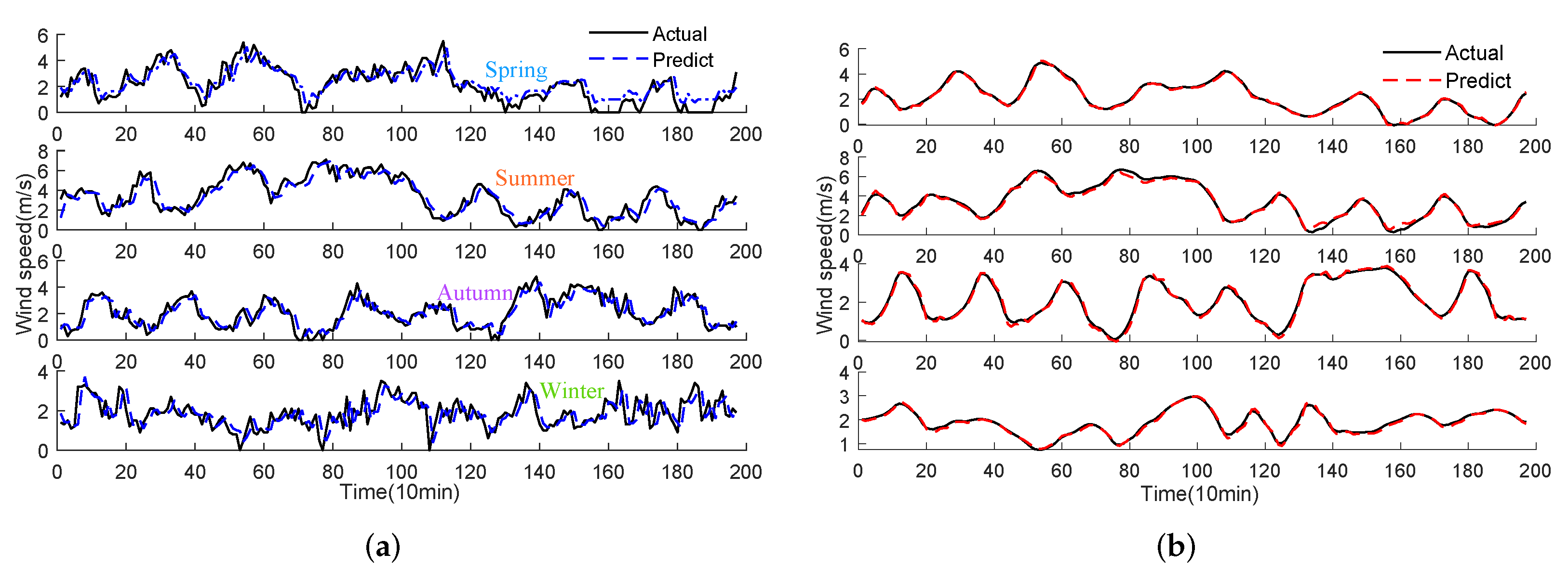
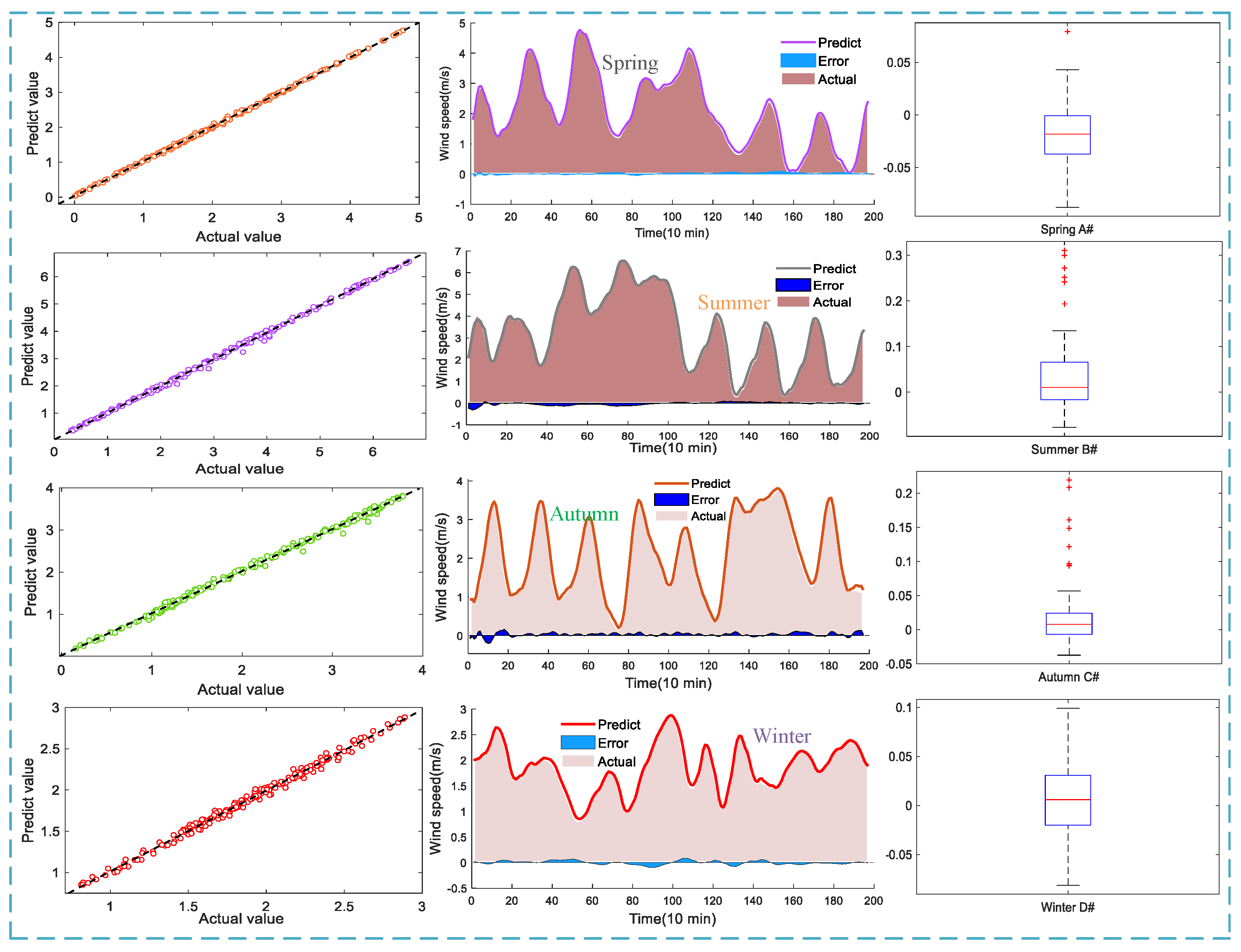
Finally, the improved GRU method strengthens the characteristic information and inline relationships of wind speed data and can comprehensively mine the characteristics of wind power, perform feature mining, and ensure the prediction accuracy and stability of the model. Four datasets in different seasons are selected for multi-step ahead prediction of the wind speed. The results show that the proposed WSTD-REMD-AVMD-DGRU model developed in this study has robust and accurate prediction performance, which can provide the best forecast results for wind series.
The present model realizes a whole adaptive process of wind speed prediction and overcomes the problems of experience adjustment, incomplete wind speed information mining, and inaccurate single-model prediction that inhibited traditional models. Moreover, the present model is robust and generalizable, which can be easily extended to time series prediction in meteorology, mechanical engineering, finance, biology, etc.

Author Contributions

Conceptualization, K.Y., B.W. and Y.L.; methodology, K.Y.; software, K.Y. and Y.W.; validation, X.Q.; formal analysis, K.Y. and Y.L.; investigation, B.W.; resources, X.Q.; data curation, J.L.; writing—original draft preparation, K.Y.; writing—review and editing, B.W.; visualization, K.Y.; supervision, J.L.; project administration, Y.L.; funding acquisition, Y.L. All authors have read and agreed to the published version of the manuscript.

Funding

This research was funded by the National Natural Science Foundation of China (Grant Nos. 91952102, 12032016, 11972220). It was also funded by Program supported by the Shanghai Education Development Foundation and the Shanghai Municipal Education Commission in China via Project (Grant No. 18SG53), as well as the Guangdong Provincial Key Laboratory under Grant No. 2019B121203001.

Institutional Review Board Statement

Not applicable.

Informed Consent Statement

Not applicable.

Conflicts of Interest

The authors declare no conflict of interest.

References

  1. Wang, Y.; Zou, R.; Liu, F.; Zhang, L.; Liu, Q. A review of wind speed and wind power forecasting with deep neural networks. Appl. Energy 2021, 304, 117766. [Google Scholar] [CrossRef]
  2. Liu, L.; Wang, Z.; Wang, Y.; Wang, J.; Chang, R.; He, G.; Tang, W. Optimizing wind/solar combinations at finer scales to mitigate renewable energy variability in China. Renew. Sustain. Energy Rev. 2020, 156, 321–330. [Google Scholar] [CrossRef]
  3. Zuluaga, D.; Alvarez, A.; Giraldo, T. Short-term wind speed prediction based on robust Kalman filtering: An experimental comparison. Appl. Energy 2015, 156, 321–330. [Google Scholar] [CrossRef]
  4. Deng, Y.; Wang, B.; Lu, Z. A hybrid model based on data preprocessing strategy and error correction system for wind speed forecasting. Energy Convers. Manag. 2020, 212, 112779. [Google Scholar] [CrossRef]
  5. Brabec, M.; Craciun, A.; Dumitrescu, A. Hybrid numerical models for wind speed forecasting. J. Atmos. Sol. Terr. Phys. 2021, 220, 105669. [Google Scholar] [CrossRef]
  6. Bouzgou, H.; Benoudjit, N. Multiple architecture system for wind speed prediction. Appl. Energy 2011, 88, 2463–2471. [Google Scholar] [CrossRef]
  7. Wang, H.; Han, S.; Liu, Y.; Yan, J.; Li, L. Sequence transfer correction algorithm for numerical weather prediction wind speed and its application in a wind power forecasting system. Appl. Energy 2019, 237, 1–10. [Google Scholar] [CrossRef]
  8. Ye, L.; Zhao, Y.; Zeng, C.; Zhang, C. Short-term wind power prediction based on spatial model. Renew. Energy 2017, 101, 1067–1074. [Google Scholar] [CrossRef]
  9. Geibel, M.; Bangga, G. Data Reduction and Reconstruction of Wind Turbine Wake Employing Data Driven Approaches. Energies 2022, 15, 3773. [Google Scholar] [CrossRef]
  10. Liang, T.; Zhao, Q.; Lv, Q.; Sun, H. A novel wind speed prediction strategy based on Bi-LSTM, MOOFADA and transfer learning for centralized control centers. Energy 2021, 230, 120904. [Google Scholar] [CrossRef]
  11. Lydia, M.; Kumar, S.; Selvakumar, A.; Kumar, G. Linear and non-linear autoregressive models for short-term wind speed forecasting. Energy Convers. Manag. 2016, 112, 115–124. [Google Scholar] [CrossRef]
  12. Erdem, E.; Shi, J. ARMA based approaches for forecasting the tuple of wind speed and direction. Appl. Energy 2011, 88, 1405–1414. [Google Scholar] [CrossRef]
  13. Valipour, M.; Banihabib, M.; Behbahani, S. Comparison of the ARMA, ARIMA, and the autoregressive artificial neural network models in forecasting the monthly inflow of Dez dam reservoir. J. Hydrol. 2013, 476, 433–441. [Google Scholar] [CrossRef]
  14. Corba, B.; Egrioglu, E.; Dalar, A. AR–ARCH type artificial neural network for forecasting. Neural Process. Lett. 2020, 51, 819–836. [Google Scholar] [CrossRef]
  15. Radziukynas, V.; Klementavicius, A. Short-term wind speed forecasting with ARIMA model. In Proceedings of the 2014 55th International Scientific Conference on Power and Electrical Engineering of Riga Technical University (RTUCON), Riga, Latvia, 14 October 2014; IEEE: Piscataway, NJ, USA, 2014; pp. 145–149. [Google Scholar]
  16. Tian, Z.; Wang, G.; Ren, Y. Short-term wind speed forecasting based on autoregressive moving average with echo state network compensation. Wind. Eng. 2020, 44, 152–167. [Google Scholar] [CrossRef]
  17. Nair, A.; Krishnaveny, R.; Vanitha, B.; Jisma, C. Forecasting of wind speed using ANN, ARIMA and hybrid models. In Proceedings of the 2017 International Conference on Intelligent Computing, Instrumentation and Control Technologies (ICICICT), Kannur, India, 6–7 July 2017; IEEE: Piscataway, NJ, USA, 2017; pp. 170–175. [Google Scholar]
  18. Shukur, O.; Lee, M. Daily wind speed forecasting through hybrid KF-ANN model based on ARIMA. Renew. Energy 2015, 76, 637–647. [Google Scholar] [CrossRef]
  19. Chen, Y.; Dong, Z.; Wang, Y.; Su, J.; Han, Z.; Zhou, D. Short-term wind speed predicting framework based on EEMD-GA-LSTM method under large scaled wind history. Energy Convers. Manag. 2021, 227, 113559. [Google Scholar] [CrossRef]
  20. Ren, C.; An, N.; Wang, J.; Li, L.; Hu, B.; Shang, D. Optimal parameters selection for BP neural network based on particle swarm optimization: A case study of wind speed forecasting. Knowl.-Based Syst. 2014, 56, 226–239. [Google Scholar] [CrossRef]
  21. Yuan, X.; Chen, C.; Yuan, Y.; Huang, Y.; Tan, Q. Short-term wind power prediction based on LSSVM–GSA model. Energy Convers. Manag. 2015, 101, 393–401. [Google Scholar] [CrossRef]
  22. Dai, F.; Nie, G.; Chen, Y. The municipal solid waste generation distribution prediction system based on FIG–GA-SVR model. J. Mater. Cycles Waste Manag. 2020, 22, 1352–1369. [Google Scholar] [CrossRef]
  23. Li, C.; Xiao, Z.; Xia, X.; Zou, W.; Zhang, C. A hybrid model based on synchronous optimisation for multi-step short-term wind speed forecasting. Appl. Energy 2018, 215, 131–144. [Google Scholar] [CrossRef]
  24. Yu, C.; Li, Y.; Zhang, M. Comparative study on three new hybrid models using Elman Neural Network and Empirical Mode Decomposition based technologies improved by Singular Spectrum Analysis for hour-ahead wind speed forecasting. Energy Convers. Manag. 2017, 147, 75–85. [Google Scholar] [CrossRef]
  25. Santhosh, M.; Venkaiah, C.; Kumar, D. Ensemble empirical mode decomposition based adaptive wavelet neural network method for wind speed prediction. Energy Convers. Manag. 2018, 168, 482–493. [Google Scholar] [CrossRef]
  26. Mora, E.; Cifuentes, J.; Marulanda, G. Short-Term Forecasting of Wind Energy: A Comparison of Deep Learning Frameworks. Energies 2021, 14, 7943. [Google Scholar] [CrossRef]
  27. Liu, H.; Chen, C. Data processing strategies in wind energy forecasting models and applications: A comprehensive review. Appl. Energy 2019, 249, 392–408. [Google Scholar] [CrossRef]
  28. Zhou, Q.; Wang, C.; Zhang, G. Hybrid forecasting system based on an optimal model selection strategy for different wind speed forecasting problems. Appl. Energy 2019, 250, 1559–1580. [Google Scholar] [CrossRef]
  29. Qian, Z.; Pei, Y.; Zareipour, H.; Chen, N. A review and discussion of decomposition-based hybrid models for wind energy forecasting applications. Appl. Energy 2019, 235, 939–953. [Google Scholar] [CrossRef]
  30. Mi, X.; Zhao, S. Wind speed prediction based on singular spectrum analysis and neural network structural learning. Energy Convers. Manag. 2020, 216, 112956. [Google Scholar] [CrossRef]
  31. Büyükşahin, Ü.Ç.; Ertekin, Ş. Improving forecasting accuracy of time series data using a new ARIMA-ANN hybrid method and empirical mode decomposition. Neurocomputing 2019, 361, 151–163. [Google Scholar] [CrossRef] [Green Version]
  32. Tian, Z.; Chen, H. Multi-step short-term wind speed prediction based on integrated multi-model fusion. Appl. Energy 2021, 298, 117248. [Google Scholar] [CrossRef]
  33. Zhang, Y.; Han, J.; Pan, G.; Xu, Y.; Wang, F. A multi-stage predicting methodology based on data decomposition and error correction for ultra-short-term wind energy prediction. J. Clean. Prod. 2021, 292, 125981. [Google Scholar] [CrossRef]
  34. Duan, J.; Wang, P.; Ma, W.; Fang, S.; Hou, Z. A novel hybrid model based on nonlinear weighted combination for short-term wind power forecasting. Int. J. Electr. Power Energy Syst. 2022, 134, 107452. [Google Scholar] [CrossRef]
  35. Liao, X.; Liu, Z.; Deng, W. Short-term wind speed multistep combined forecasting model based on two-stage decomposition and LSTM. Wind. Energy 2021, 24, 991–1012. [Google Scholar] [CrossRef]
  36. Liu, B.; Zhao, S.; Yu, X.; Zhang, L.; Wang, Q. A Novel Deep Learning Approach for Wind Power Forecasting Based on WD-LSTM Model. Energies 2020, 13, 4964. [Google Scholar] [CrossRef]
  37. Lu, P.; Ye, L.; Zhao, Y.; Dai, B.; Pei, M.; Tang, Y. Review of meta-heuristic algorithms for wind power prediction: Methodologies, applications and challenges. Appl. Energy 2021, 301, 117446. [Google Scholar] [CrossRef]
  38. Bai, Y.; Liu, M.; Ding, L.; Ma, Y. Double-layer staged training echo-state networks for wind speed prediction using variational mode decomposition. Appl. Energy 2021, 301, 117461. [Google Scholar] [CrossRef]
  39. Wu, C.; Wang, J.; Chen, X.; Du, P.; Yang, W. A novel hybrid system based on multi-objective optimization for wind speed forecasting. Renew. Energy 2020, 146, 149–165. [Google Scholar] [CrossRef]
  40. Neshat, M.; Nezhad, M.; Abbasnejad, E.; Mirjalili, S.; Tjernberg, L.; Garcia, D.; Alexander, B.; Wagner, M. A deep learning-based evolutionary model for short-term wind speed forecasting: A case study of the Lillgrund offshore wind farm. Energy Convers. Manag. 2021, 236, 114002. [Google Scholar] [CrossRef]
  41. Tian, Z.; Chen, H. A novel decomposition-ensemble prediction model for ultra-short-term wind speed. Energy Convers. Manag. 2021, 248, 114775. [Google Scholar] [CrossRef]
  42. Huang, N.; Shen, Z.; Long, S.; Wu, M.; Shih, H.; Zheng, Q.; Yen, N.; Tung, C.; Liu, H. The empirical mode decomposition and the Hilbert spectrum for nonlinear and non-stationary time series analysis. Proc. R. Soc. Lond. Ser. Math. Phys. Eng. Sci. 1998, 454, 903–995. [Google Scholar] [CrossRef]
  43. Tian, Z.; Li, S.; Wang, Y. A prediction approach using ensemble empirical mode decomposition-permutation entropy and regularized extreme learning machine for short-term wind speed. Wind. Energy 2020, 23, 177–206. [Google Scholar] [CrossRef]
  44. Wu, Z.; Xia, X.; Xiao, L.; Liu, Y. Combined model with secondary decomposition-model selection and sample selection for multi-step wind power forecasting. Appl. Energy 2020, 261, 114345. [Google Scholar] [CrossRef]
  45. Peng, Z.; Peng, S.; Fu, L.; Lu, B.; Tang, J.; Wang, K.; Li, W. A novel deep learning ensemble model with data denoising for short-term wind speed forecasting. Energy Convers. Manag. 2020, 207, 112524. [Google Scholar] [CrossRef]
  46. Liu, Z.; Peng, D.; Zuo, M.; Xia, J.; Qin, Y. Improved Hilbert–Huang transform with soft sifting stopping criterion and its application to fault diagnosis of wheelset bearings. ISA Trans. 2021, 21, 0019–0578. [Google Scholar] [CrossRef] [PubMed]
  47. Zhu, A.; Xu, C.; Li, Z.; Wu, J.; Liu, Z. Hybridizing grey wolf optimization with differential evolution for global optimization and test scheduling for 3D stacked SoC. J. Syst. Eng. Electron. 2015, 26, 317–328. [Google Scholar] [CrossRef]
  48. Dragomiretskiy, K.; Zosso, D. Variational mode decomposition. IEEE Trans. Signal Process. 2013, 62, 531–544. [Google Scholar] [CrossRef]
  49. Shivam, K.; Tzou, J.; Wu, S. Multi-Step Short-Term Wind Speed Prediction Using a Residual Dilated Causal Convolutional Network with Nonlinear Attention. Energies 2020, 13, 1772. [Google Scholar] [CrossRef] [Green Version]
Figure 1. Overall block diagram of the proposed combined model.
Energies 15 04221 g001
Figure 2. Basic information of the four datasets used in this study.
Energies 15 04221 g002
Figure 3. The four datasets denoised by WSTD. The vertical dashed lines denote the separation of training data and test data.
Energies 15 04221 g003
Figure 4. The hierarchy of the grey wolf pack.
Energies 15 04221 g004
Figure 5. GRU structure.
Energies 15 04221 g005
Figure 6. Comparison of BPNN prediction results of four wind speed series with and without denoising: (a) without the WSTD denoising; (b) with the WSTD denoising.
Energies 15 04221 g006
Figure 7. REMD decomposition results of the four wind speed series. (AD) are REMD decomposition results of four datasets in spring, summer, autumn and winter respectively.
Energies 15 04221 g007
Figure 8. Heat map of Spearman correlation coefficients between the original wind speed series from dataset C and each IMF from the REMD.
Energies 15 04221 g008
Figure 9. Combination of K and α parameters after AVMD. A, B, C and D are the combined parameters of AVMD decomposition of the four datasets in spring, summer, autumn and winter respectively.
Energies 15 04221 g009
Figure 10. Single-step prediction results of the four wind speed series.
Energies 15 04221 g010
Figure 11. The prediction results on the dataset C.
Energies 15 04221 g011
Figure 12. Error probability plot of multi-step prediction for the WSTD-REMD-AVMD-DGRU model. (AD) are the prediction error probability plot of four data sets in spring, summer, autumn and winter respectively.
Energies 15 04221 g012
Table 1. Comparison of WT with various wavelet basis functions.
Wavelet Basis FunctionSNR/dBRMSE
db412.85880.5677
haar11.33180.6768
db312.51650.5905
sym212.34920.6020
Table 2. The performance evaluation index.
IndexMeaningEquation
SNRSignal-to-noise ratio S N R = 101 g ( i = 1 N y i 2 i = 1 N ( y i y i ^ ) 2 )
MAEMean absolute error M A E = 1 N i = 1 N | y i y i ^ |
RMSERoot mean square error R M S E = 1 N i = 1 N ( y i y i ^ ) 2
R 2 Coefficient of determination R 2 = 1 i = 1 N ( y i y i ^ ) 2 i = 1 N ( y i y ^ ) 2
TICTheil inequality coefficient T I C = 1 N t = 1 N ( y i y i ^ ) 2 1 N t = 1 N y i 2 + 1 N t = 1 N y i ^ 2
SSESquare sum error S S E = i = 1 N ( y i y i ^ ) 2
Table 3. The prediction performance from various models on dataset A.
Model MAE RMSE R 2 TIC SSE
1-Step2-Step3-Step1-Step2-Step3-Step1-Step2-Step3-Step1-Step2-Step3-Step1-Step2-Step3-Step
The proposed0.0265 0 . 0531 0 . 0818 0 . 0338 0 . 0782 0 . 1273 0 . 9986 0 . 9957 0 . 9875 0 . 0080 0 . 0283 0 . 0296 0 . 0098 0 . 0184 0 . 0330
WSTD-VMD-HGWO-SVR0.08730.09970.11050.09360.12030.13460.99420.99370.99020.02460.02870.03960.56481.62432.6591
WSTD-REMD-HGWO-GRU0.10820.13940.17720.12570.16780.21770.99140.98210.97010.02960.03970.05152.31574.91757.8733
WSTD-CEEMD-HGWO-GRU0.23810.32420.43170.31120.46620.58260.94590.87410.80500.07350.11060.137416.292339.268657.5463
WSTD-REMD-GWO-GRU0.20290.21510.22660.24590.25690.27450.97400.96620.95950.05660.05970.06476.28629.96389.2274
WSTD-REMD-HGWO-SVR0.14820.15540.48010.23640.28880.58930.97520.94610.77570.05420.06780.14177.397016.100059.1824
WSTD-WD-GWO-SVR0.16310.26240.33810.20620.34300.44120.97580.93110.88290.04930.08090.10467.795820.785234.2191
WSTD-VMD–GRU0.02890.09680.10450.04140.09160.13890.99700.99250.98660.01080.02190.03420.26660.95483.5586
WSTD-CEEMD-GRU0.22560.27600.32550.31900.36050.38170.93660.92030.91320.07480.08500.088819.723825.566327.3503
WSTD-WD-GRU0.25370.30610.47510.33800.40510.59110.93420.90580.80110.08260.09590.131422.503232.164868.1359
VMD-HGWO-SVR0.13510.17860.17760.16340.21570.21600.98700.97740.97240.03830.05020.05093.34646.62537.0425
WD-HGWO-SVR0.16340.26160.33540.20630.33960.43510.98670.93380.89170.04890.07990.10288.381822.609736.9103
WSTD-REMD-GRU0.05100.15570.17250.06720.18830.24060.99700.98630.96540.01590.044330.05800.87344.04789.9962
WSTD-GWO-SVR0.20020.21380.22580.24270.25600.27030.97320.96680.95770.05600.05950.06366.51647.811010.0248
GRU0.51000.67240.78340.65970.85460.98840.76730.60780.48530.15410.19890.226255.392670.793869.7912
LSTM0.50220.68010.77330.65150.87350.97010.77370.59420.49430.15260.20240.224153.083768.510279.3900
ARIMA0.50560.65500.76550.64500.82050.95350.77220.63360.50840.15250.19300.223159.512174.040076.1862
BP0.51530.63760.75780.65970.83940.94400.76320.61560.51910.15570.20150.221358.447482.870174.1387
LSSVM0.51190.66160.75960.64990.82920.95380.77240.63170.52020.15370.19510.223353.987365.139261.5543
RF0.57140.74920.87940.71900.93241.09290.71780.53250.36420.17000.21760.256279.6895109.9353119.3138
Table 4. The prediction performance from various models on dataset B.
Model MAE RMSE R 2 TIC SSE
1-Step2-Step3-Step1-Step2-Step3-Step1-Step2-Step3-Step1-Step2-Step3-Step1-Step2-Step3-Step
The proposed 0 . 0534 0 . 0748 0 . 0856 0 . 0758 0 . 1036 0 . 1246 0 . 9987 0 . 9977 0 . 9969 0 . 0115 0 . 0157 0 . 0173 0 . 7567 2 . 1019 2 . 5629
WSTD-VMD-HGWO-SVR0.13900.15180.16260.17880.18610.20100.99010.98910,98430.02700.02790.03016.03894.95235.7395
WSTD-REMD-HGWO-GRU0.19520.24540.31400.23870.30390.40960.98580.97300.94790.03600.04560.06117.856015.275630.4725
WSTD-CEEMD-HGWO-GRU0.28910.35310.48670.36970.45520.60760.96130.94430.89930.05550.06880.091324.864232.880454.8275
WSTD-REMD-GWO-GRU0.19720.21170.29520.23320.39470.49500.98950.95380.92320.03500.06030.07455.557027.467847.3507
WSTD-REMD-HGWO-SVR0.26490.38180.45640.31850.47510.55830.97150.93540.91080.04740.07070.083118.795339.971853.7150
WSTD-WD-GWO-SVR0.40100.40730.40790.47350.47830.48500.96390.96200.96180.07230.07350.074614.931415.361815.3963
WSTD-VMD–GRU0.13870.20000.28490.18100.21600.55250.99340.98490.90780.02780.03250.08263.08328.800559.2937
WSTD-CEEMD-GRU0.39690.51270.66380.64300.95661.05100.92340.83930.82880.10130.15130.172859.4176156.9631170.2382
WSTD-WD-GRU0.28930.39050.52510.39940.51340.64000.95440.92500.88410.05970.07650.099031.428051.658279.8677
VMD-HGWO-SVR0.23290.39860.42420.31780.41000.53650.97200.96890.93120.04720.05140.07636.934223.792336.5286
WD-HGWO-SVR0.26910.38720.45140.32490.48090.55440.97010.93420.91300.04840.07150.082420.803945.335659.9384
WSTD-REMD-GRU0.11970.20830.34100.16000.31500.44400.99450.97600.88130.02430.04640.10523.496016.653834.7916
WSTD-GWO-SVR0.39830.40480.41080.47510.48020.48580.96540.96330.96360.07260.07330.073614.147214.785614.4973
GRU0.53020.70810.87220.68190.91431.12750.87220.77220.65660.10320.13900.173175.5531114.9054160.5826
LSTM0.56490.81800.93250.74851.01201.17520.84530.72750.63050.11270.15600.176699.0382127.8319213.4905
ARIMA0.51250.76780.95720.72330.97301.17230.85420.73960.62360.10870.14620.177688.6792151.3385184.1856
BP0.64980.77370.96240.81090.96601.17170.84350.74970.62390.12510.14780.178069.9745117.8563175.6531
LSSVM0.59500.79530.98200.74680.98491.18700.84800.73620.61790.11300.14980.181782.4907123.8675152.3672
RF0.65880.85081.01540.83971.06701.25440.80690.68980.57530.12770.16280.1929106.3476161.5313188.5835
Table 5. The prediction performance from various models on dataset C.
Model MAE RMSE R 2 TIC SSE
1-Step2-Step3-Step1-Step2-Step3-Step1-Step2-Step3-Step1-Step2-Step3-Step1-Step2-Step3-Step
The proposed0.0440 0 . 0459 0 . 0462 0 . 0582 0 . 0615 0 . 0626 0 . 9983 0 . 9967 0 . 9921 0 . 0138 0 . 0146 0 . 0149 0 . 5298 0 . 7387 0 . 7675
WSTD-VMD-HGWO-SVR0.08650.09010.11660.10470.11380.14580.98950.98870.98210.02500.02700.03431.96702.13973.2653
WSTD-REMD-HGWO-GRU0.09910.16400.21860.12430.20130.27240.98790.96470.93130.02940.04750.06422.54697.429313.6527
WSTD-CEEMD-HGWO-GRU0.19710.40870.41180.26050.50050.51590.93720.80140.78350.06270.11790.123014.635841.923248.0972
WSTD-REMD-GWO-GRU0.14500.16100.16150.17450.19310.19710.98060.97510.97090.04060.04500.04623.75924.74905.4628
WSTD-REMD-HGWO-SVR0.13070.20250.20950.18080.26260.26070.97770.94820.93030.04240.06130.06184.823111.643812.9346
WSTD-WD-GWO-SVR0.16110.27120.36140.21000.34560.44500.96670.90410.83890.04810.08160.10437.507319.463532.5792
WSTD-VMD–GRU0.02260.06780.09520.03700.06280.17850.99880.99670.96910.00890.01490.04240.24040.63096.1653
WSTD-CEEMD-GRU0.07760.19570.25320.12720.38120.44560.98480.86440.82880.03040.09160.10643.193731.418638.9903
WSTD-WD-GRU0.22120.24270.53990.32110.31550.73300.91480.91790.55670.07850.07730.173820.307619.5159104.7591
VMD-HGWO-SVR0.11490.14560.16800.14200.17650.20530.98940.97810.96400.03480.04310.04962.13904.28466.6573
WD-HGWO-SVR0.16630.27570.36110.21110.35630.44480.96320.92710.83670.05040.08390.10428.781324.882338.5802
WSTD-REMD-GRU0.08700.18130.21410.12240.22660.31630.98830.96530.90870.02890.05260.07612.41387.102519.0146
WSTD-GWO-SVR0.16120.15990.15040.19680.19210.18190.97130.97580.98010.04610.04470.04225.39704.56783.8964
GRU0.45710.53680.60110.58440.68700.77260.73500.63450.53860.14050.16370.185949.526755.258963.1174
LSTM0.45240.52460.59160.57880.66200.74390.74020.66150.57160.13840.15770.176046.567261.748360.8625
ARIMA0.47850.58950.69830.60280.74290.86100.71800.57220.42570.14450.17820.206052.922660.723459.1549
BP0.47780.59020.69300.61060.74470.85800.71420.56990.43210.14800.17820.206756.936863.328755.3472
LSSVM0.48180.59730.71480.60300.74870.87090.71780.56410.41220.14430.17890.207250.096761.745363.9388
RF0.53190.69970.81220.68060.89101.02850.64710.41230.25030.16460.21630.249668.885094.6278107.4784
Table 6. The prediction performance from various models on dataset D.
Model MAE RMSE R 2 TIC SSE
1-Step2-Step3-Step1-Step2-Step3-Step1-Step2-Step3-Step1-Step2-Step3-Step1-Step2-Step3-Step
The proposed0.0309 0 . 0374 0 . 0444 0 . 0384 0 . 0467 0 . 0562 0 . 9973 0 . 9945 0 . 9873 0 . 0101 0 . 0124 0 . 0150 0 . 2902 0 . 4274 0 . 6168
WSTD-VMD-HGWO-SVR0.04330.06630.08910.05220.08240.11010.99160.98080.96720.01390.02190.02910.48501.06141.7848
WSTD-REMD-HGWO-GRU0.04360.07160.09050.05400.09040.12130.98860.96890.94530.01450.02430.03260.54241.39342.1183
WSTD-CEEMD-HGWO-GRU0.26090.26670.33270.35480.35850.47420.70730.70180.53170.09570.09410.124818.628620.342935.7302
WSTD-REMD-GWO-GRU0.06590.08600.11200.08310.10570.13680.97550.95660.93720.02230.02840.03711.01291.95402.7816
WSTD-REMD-HGWO-SVR0.16470.12840.19450.24720.31760.35040.88090.69580.65930.06330.08450.09106.775219.678321.3897
WSTD-WD-GWO-SVR0.14420.21720.26820.18700.29650.35250.91910.79410.71110.05020.07930.09465.814713.151818.5134
WSTD-VMD–GRU0.08530.09520.27030.22170.24250.52230.81050.78380.44700.05950.06510.13979.546211.523853.1585
WSTD-CEEMD-GRU0.14670.23850.27180.41630.56550.63230.58130.33500.23270.11030.15180.171534.662890.1783137.5041
WSTD-WD-GRU0.21990.27850.32470.32900.36850.40630.74600.68010.61340.08770.09890.109326.756321.218032.1939
VMD-HGWO-SVR0.06100.08880.11990.07600.11310.15430.98760.95420.92060.02040.03850.04070.57071.83362.8740
WD-HGWO-SVR0.14410.21730.26170.18600.29660.34050.91860.79360.71890.04980.07920.09286.813717.246923.4062
WSTD-REMD-GRU0.04910.12580.14370.10490.21510.28200.95680.85950.73160.02810.05610.07482.14477.476215.1173
WSTD-GWO-SVR0.06700.08430.11010.08400.10450.13580.97550.95730.93800.02250.02810.03681.01381.92952.7120
GRU0.44480.54700.60110.58830.69570.73950.65460.55670.43470.15580.18240.190835.852437.356240.5836
LSTM0.44900.55020.58090.59290.69350.72610.64360.55710.49120.15700.18000.190436.907836.684535.8163
ARIMA0.45110.53590.58500.60120.69550.73900.54790.46170.35260.15960.18340.192143.986742.932137.8196
BP0.45320.54190.57600.60070.69460.71720.54540.47390.30150.16000.18120.191442.967243.837336.1058
LSSVM0.44230.52550.57450.58610.67980.71940.46010.37720.29280.15550.17930.188637.852139.038532.8654
RF0.52830.58630.61790.68260.74810.79850.57580.44550.35920.18060.19680.208263.267865.975666.6372
Publisher’s Note: MDPI stays neutral with regard to jurisdictional claims in published maps and institutional affiliations.

