
Computation and Analysis of an Offshore Wind Power Forecast: Towards a Better Assessment of Offshore Wind Power Plant Aerodynamics

 ,
,
Abstract
:
1. Introduction
2. Literature Review
- 1.
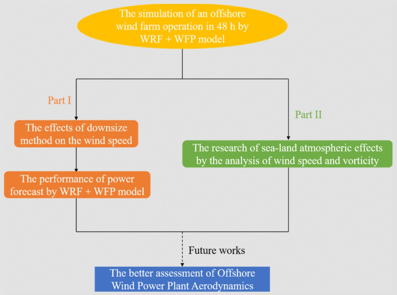
- The accuracy of simulating the wind speed and power production is validated, including the performance of the downsizing method in the different locations inside the wind farm.
- 2.
- The transition from the sea to the land has some impacts on the simulation of the flow field in the area near the coastline, and these influences are discussed. Moreover, except for the velocity, the variations of vorticity are taken into consideration.
3. Research Methods
3.1. Description of the Mathematical Model
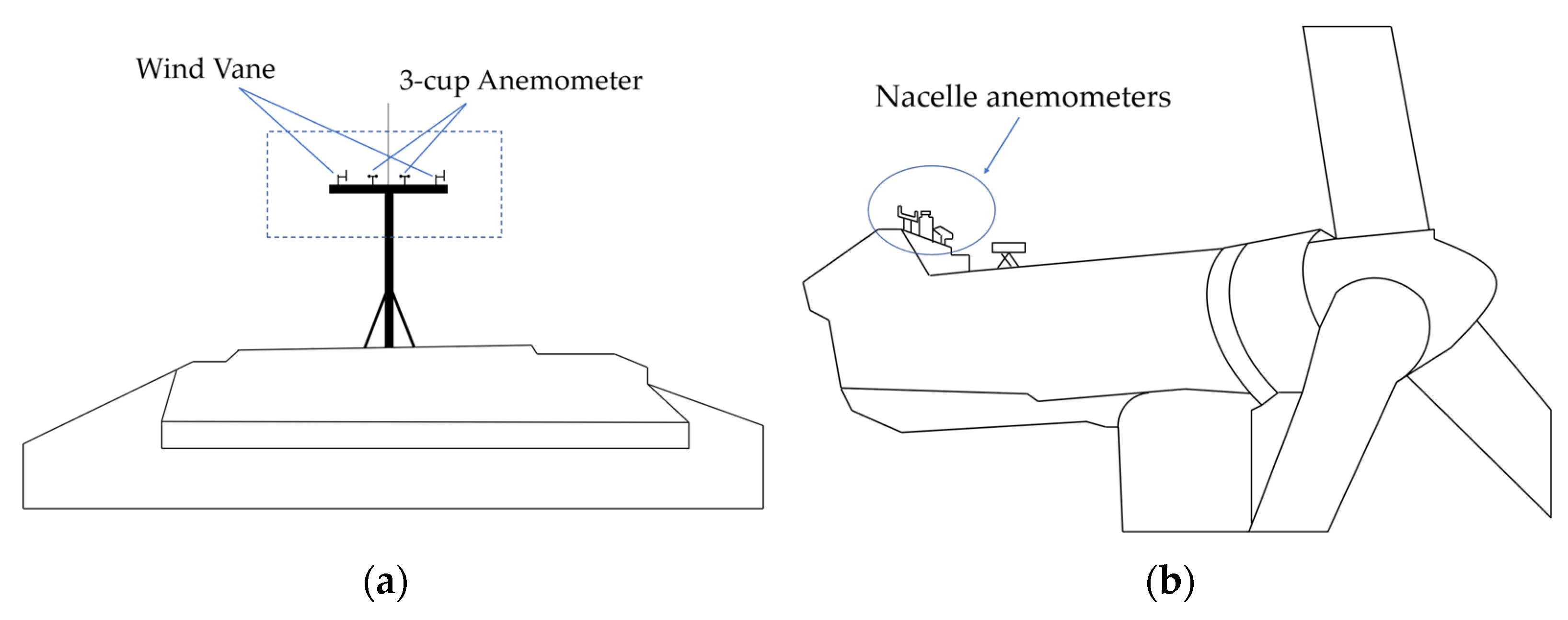
3.2. Measurements
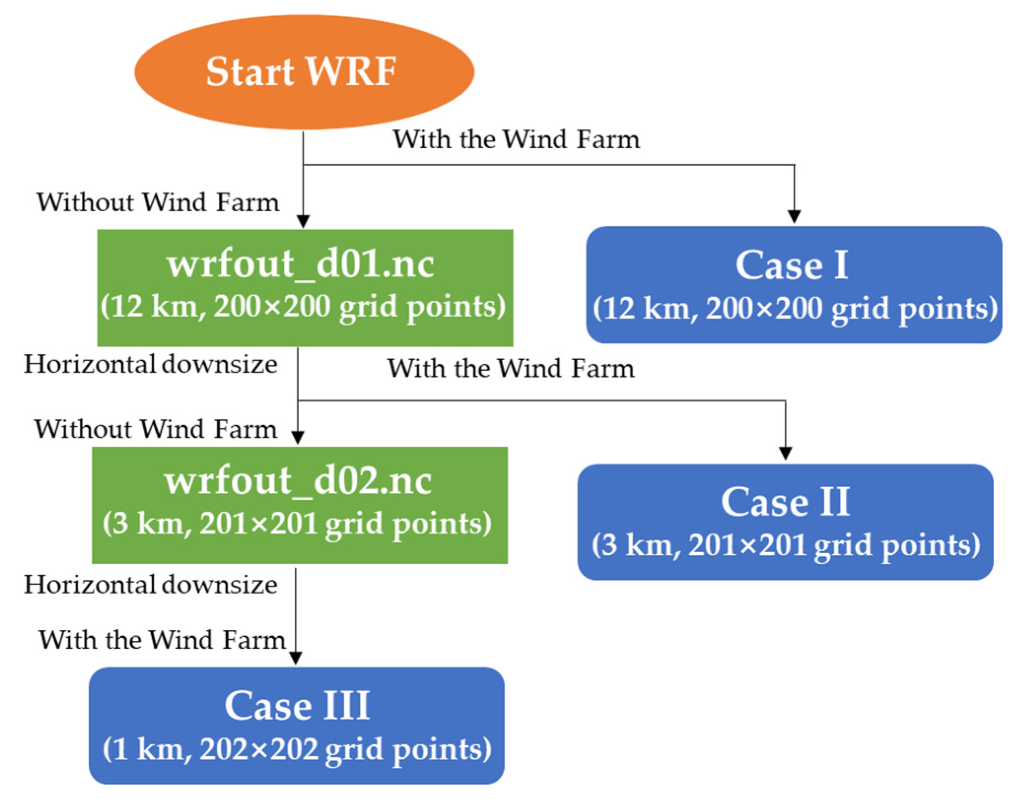
3.3. Simulation Methods
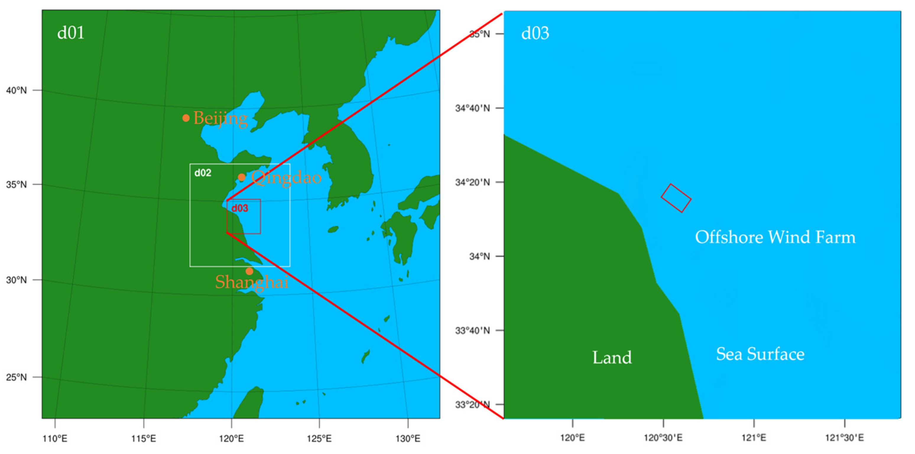
4. Study Area
5. Results
5.1. Performance of Wind Speed and Power Simulations
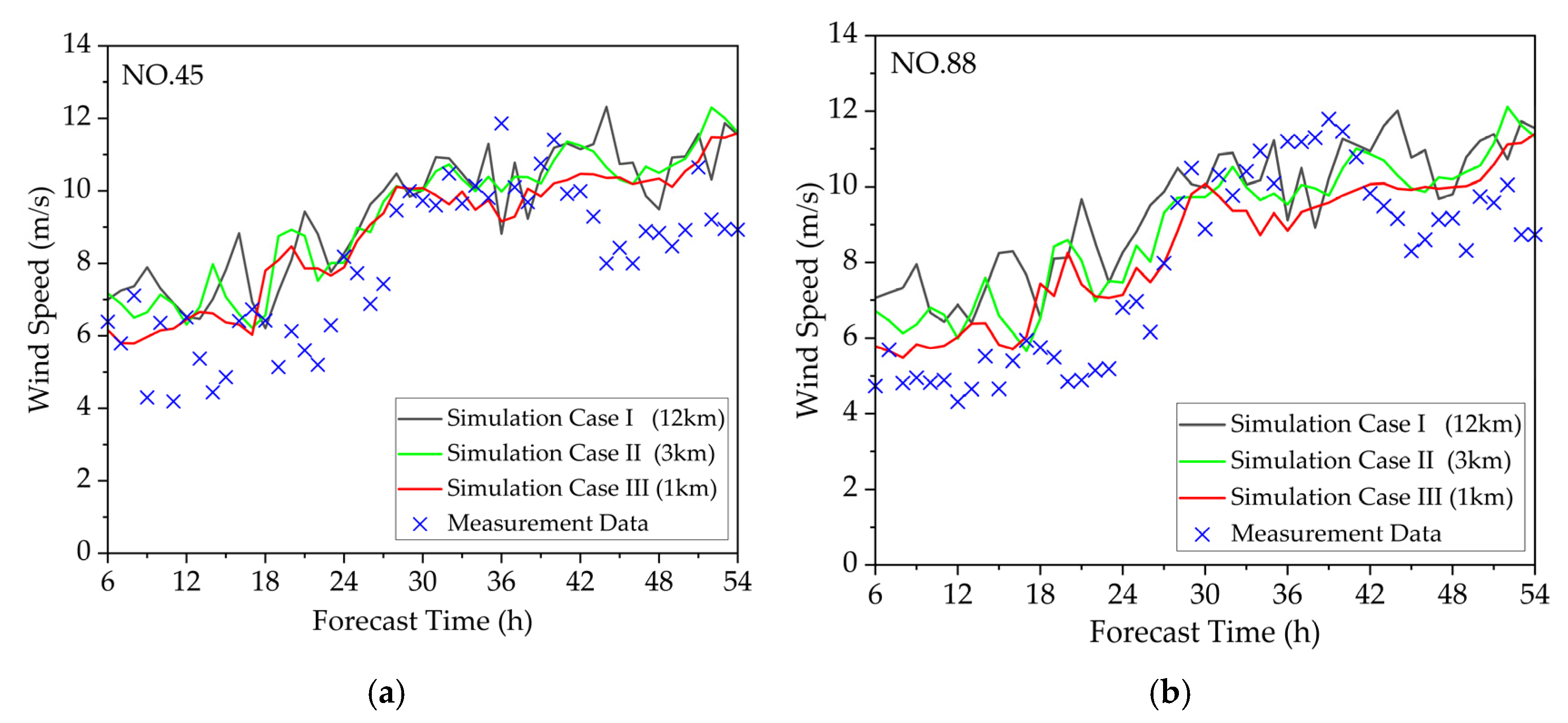
5.1.1. Wind Speed Simulation on the Hub Height
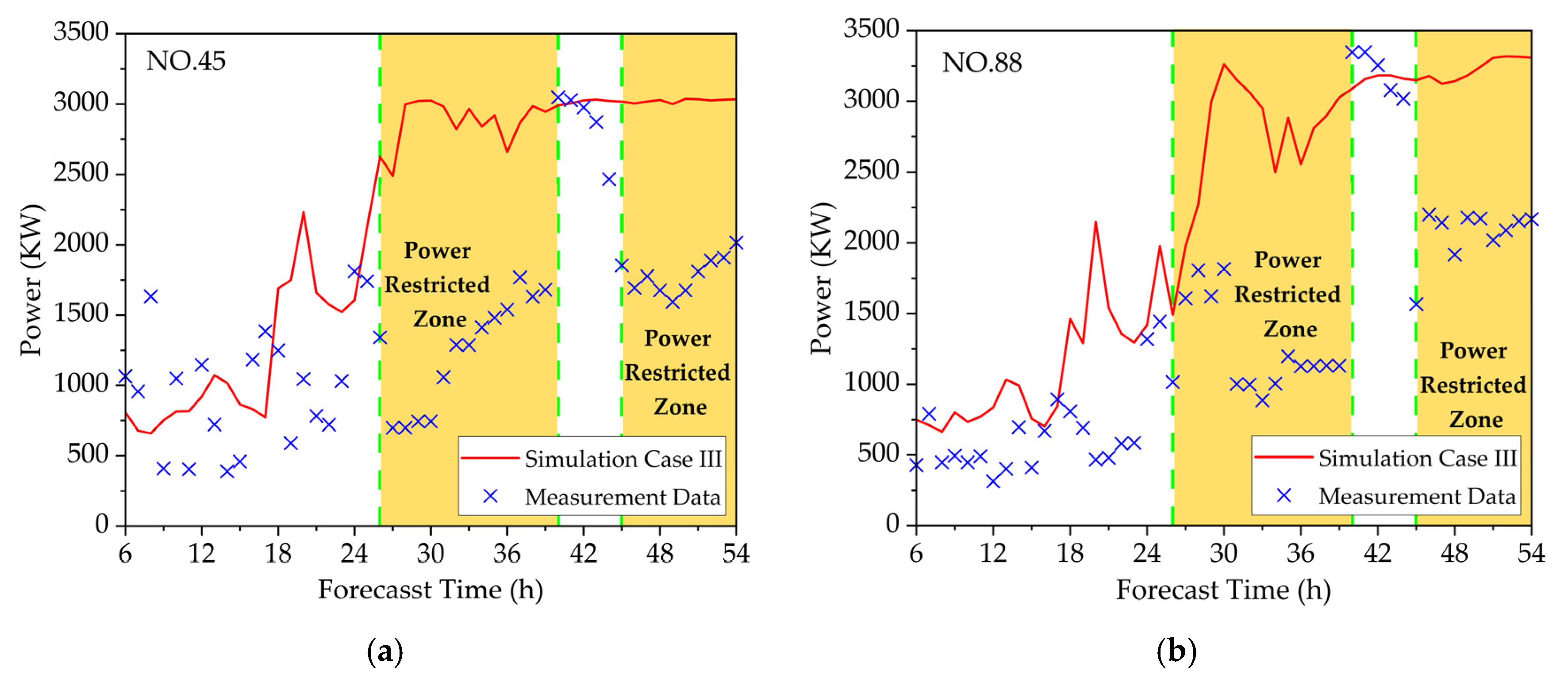
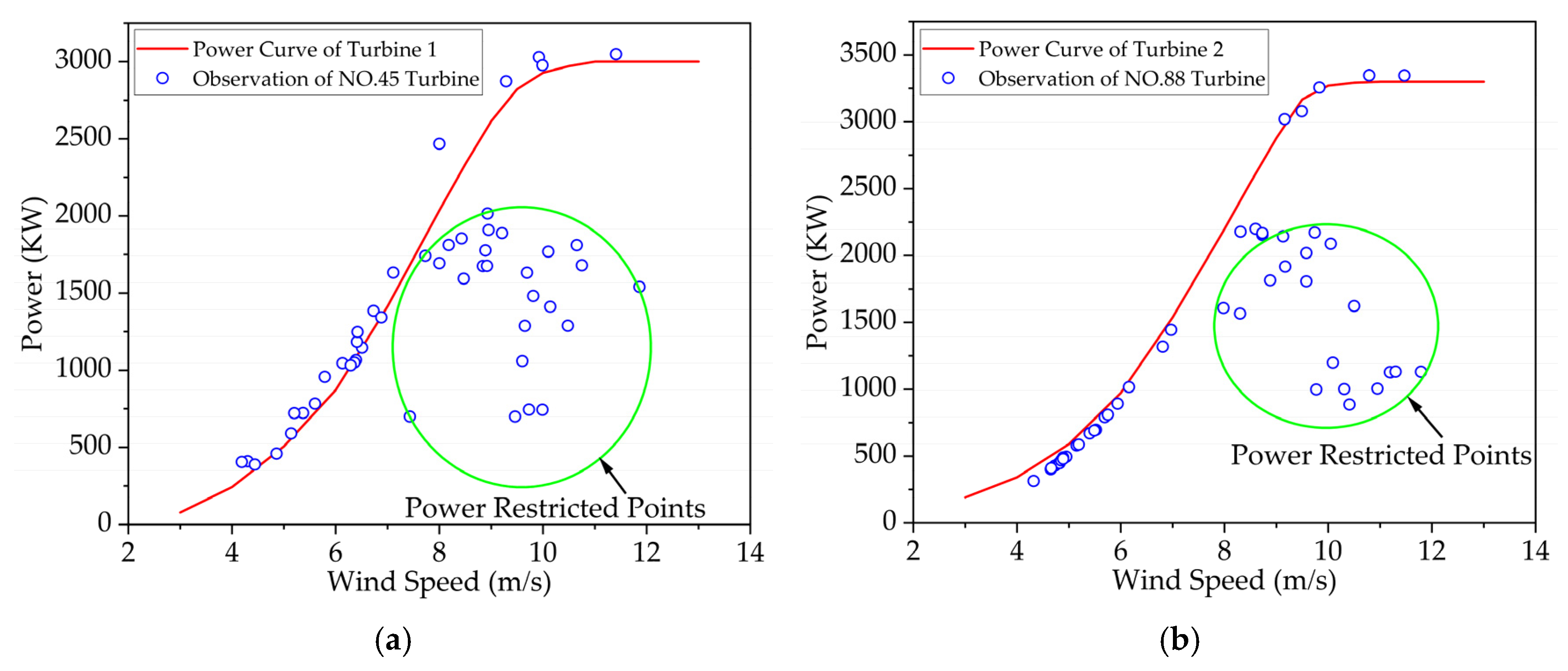
5.1.2. Turbine Power Forecast
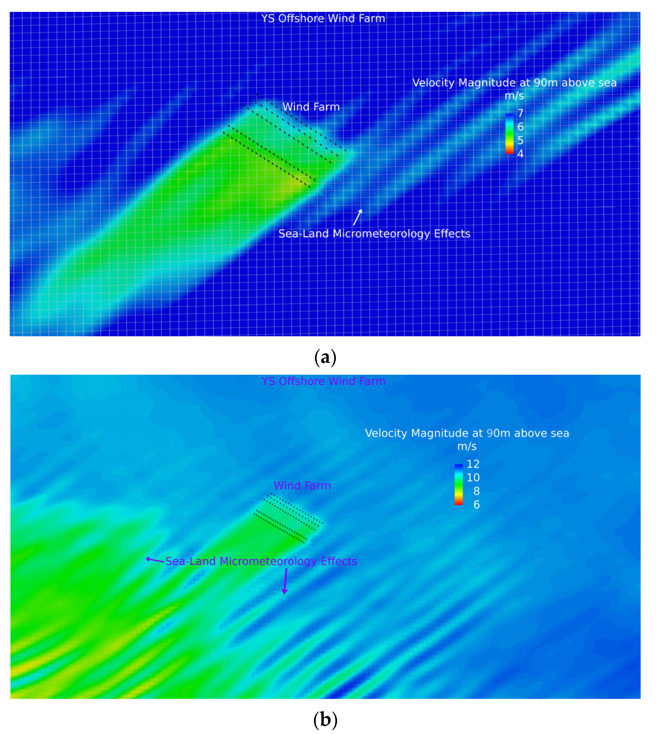
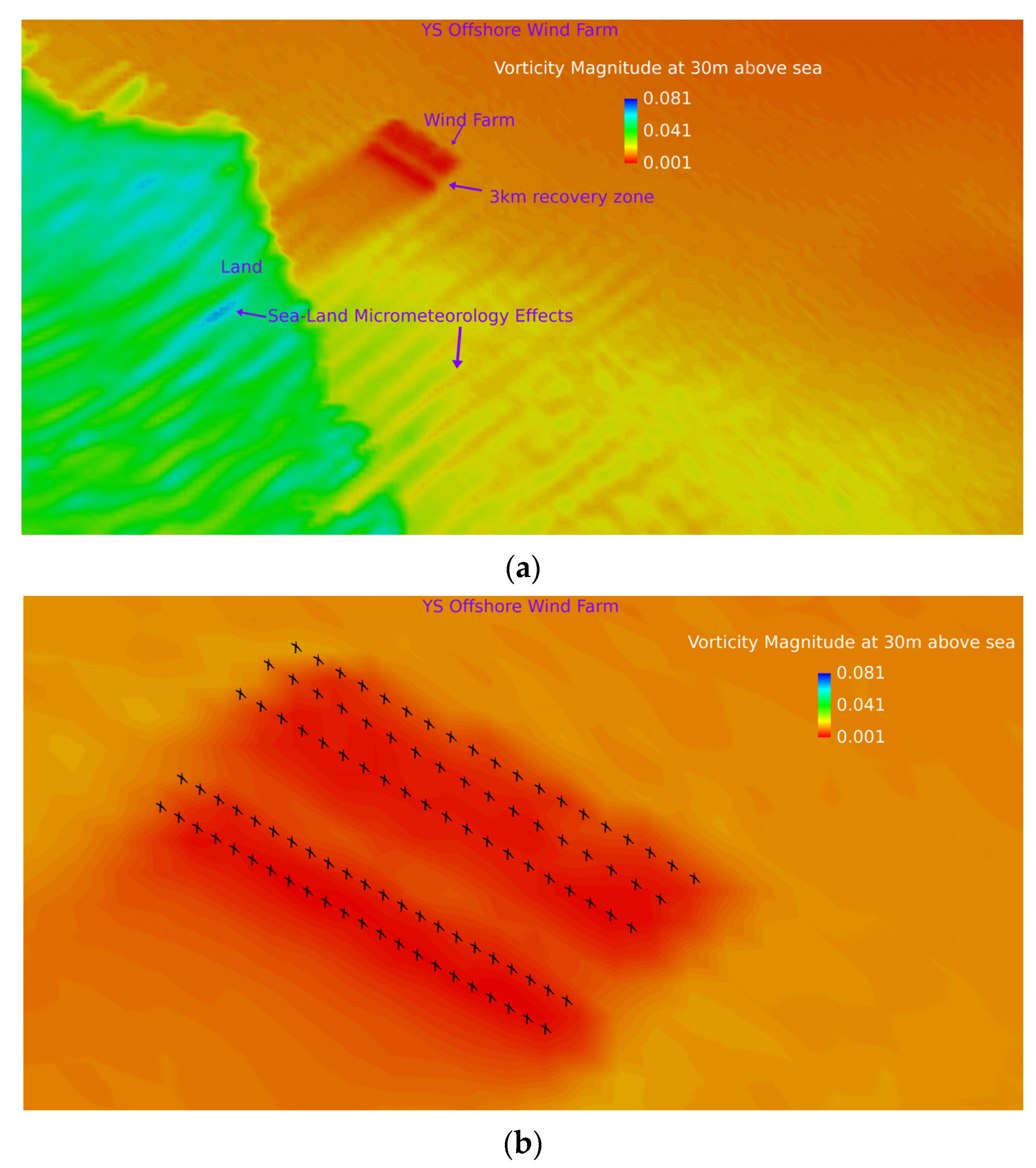
5.2. Sea–Land Atmospheric Effects and Vorticity in the Model
6. Discussion
6.1. Discussion of Wind Speed and Power Simulations
6.2. Discussion of Sea–Land Atmospheric Effects and Vorticity
7. Summary
Author Contributions
Funding
Institutional Review Board Statement
Informed Consent Statement
Data Availability Statement
Acknowledgments
Conflicts of Interest
Abbreviations
| CFD | Computational Fluid Dynamics |
| GFS | Global Forecast System |
| LES | Large Eddy Simulation |
| MYNN | Mellor–Yamada–Nakanishi–Niino model |
| NECP | National Centers for Environmental Prediction |
| NREL | National Renewable Energy Laboratory |
| PBL | Planet Boundary Layer |
| RMSE | Root Mean Squared Error |
| SCADA | Supervisory Control and Data Acquisition System |
| SVR | Support Vector Regression |
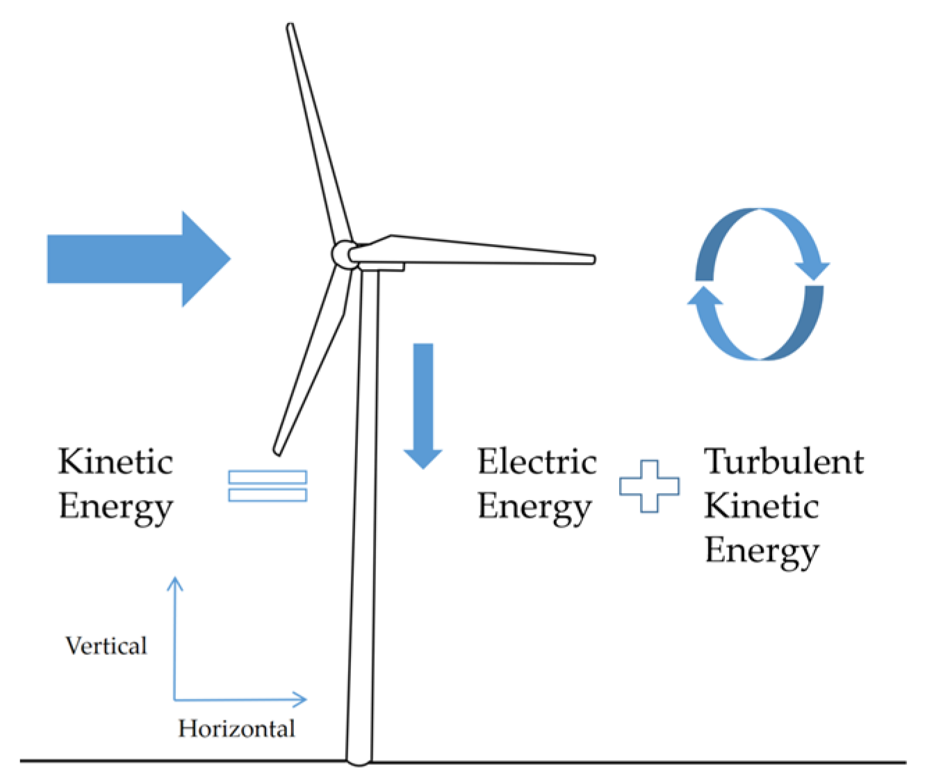
| TKE | Turbulence Kinetic Energy |
| UTC | Universal Time Coordinated |
| WFP | Wind Farm Parameterization |
| WRF | Weather Research and Forecast Model |
References
- Global Wind Energy Council (GWEC). Global Wind Report 2021. Available online: https://gwec.net/wp-content/uploads/2021/03/GWEC-Global-Wind-Report-2021.pdf (accessed on 27 October 2021).
- Veers, P.; Dykes, K.; Lantz, E.; Barth, S.; Bottasso, C.L.; Carlson, O.; Clifton, A.; Green, J.; Green, P.; Holttinen, H.; et al. Grand challenges in the science of wind energy. Science 2019, 366, 6464. [Google Scholar] [CrossRef] [Green Version]
- Jung, J.; Broadwater, R.P. Current status and future advances for wind speed and power forecasting. Renew. Sustain. Energy Rev. 2014, 31, 762–777. [Google Scholar] [CrossRef]
- Hanifi, S.; Liu, X.; Lin, Z.; Lotfian, S. A Critical Review of Wind Power Forecasting Methods—Past, Present and Future. Energies 2020, 13, 3764. [Google Scholar] [CrossRef]
- Marugán, A.P.; Márquez, F.P.G.; Perez, J.M.P.; Ruiz-Hernández, D. A survey of artificial neural network in wind energy systems. Appl. Energ. 2018, 228, 1822–1836. [Google Scholar] [CrossRef] [Green Version]
- Zendehboudi, A.; Baseer, M.A.; Saidur, R. Application of support vector machine models for forecasting solar and wind energy resources: A review. J. Clean. Prod. 2018, 199, 272–285. [Google Scholar] [CrossRef]
- Ren, C.; An, N.; Wang, J.; Li, L.; Hu, B.; Shang, D. Optimal parameters selection for BP neural network based on particle swarm optimization: A case study of wind speed forecasting. Knowl.-Based. Syst. 2014, 56, 226–239. [Google Scholar] [CrossRef]
- Zameer, A.; Arshad, J.; Khan, A.; Raja, M.A.Z. Intelligent and robust prediction of short term wind power using genetic programming based ensemble of neural networks. Energy Convers. Manag. 2017, 134, 361–372. [Google Scholar] [CrossRef]
- Li, L.; Zhao, X.; Tseng, M.; Tan, R.R. Short-term wind power forecasting based on support vector machine with improved dragonfly algorithm. J. Clean. Prod. 2020, 242, 118447. [Google Scholar] [CrossRef]
- Dhiman, H.S.; Deb, D.; Balas, V.E. Supervised Machine Learning in Wind Forecasting and Ramp Event Prediction; Academic Press: Cambridge, MA, USA, 2020. [Google Scholar] [CrossRef]
- Dhiman, H.S.; Anand, P.; Deb, D. Wavelet transform and variants of SVR with application in wind forecasting. In Innovations in Infrastructure; Springer: Singapore, 2019; pp. 501–511. [Google Scholar] [CrossRef]
- Dhiman, H.S.; Deb, D. Machine intelligent and deep learning techniques for large training data in short-term wind speed and ramp event forecasting. Int. Trans. Electr. Energ. Syst. 2021, 31, e12818. [Google Scholar] [CrossRef]
- Dhiman, H.S.; Deb, D.; Foley, A.M. Bilateral Gaussian Wake Model Formulation for Wind Farms: A Forecasting based approach. Renew. Sustain. Energy Rev. 2020, 127, 109873. [Google Scholar] [CrossRef]
- Bieda, A.; Cienciała, A. Towards a Renewable Energy Source Cadastre—A Review of Examples from around the World. Energies 2021, 14, 8095. [Google Scholar] [CrossRef]
- Lehneis, R.; Manske, D.; Thrän, D. Modeling of the German Wind Power Production with High Spatiotemporal Resolution. ISPRS Int. J. Geo-Inf. 2021, 10, 104. [Google Scholar] [CrossRef]
- Porté-Agel, F.; Bastankhah, M.; Shamsoddin, S. Wind-Turbine and Wind-Farm Flows: A Review. Bound.-Layer Meteorol. 2020, 174, 1–59. [Google Scholar] [CrossRef] [Green Version]
- Keith, D.W.; Decarolis, J.F.; Denkenberger, D.C.; Lenschow, D.H.; Malyshev, S.L.; Pacala, S.; Rasch, P.J. The influence of large-scale wind power on global climate. Proc. Natl. Acad. Sci. USA 2004, 101, 16115–16120. [Google Scholar] [CrossRef] [Green Version]
- Kirk-Davidoff, D.B.; Keith, D.W. On the Climate Impact of Surface Roughness Anomalies. J. Atmos. Sci. 2008, 65, 2215–2234. [Google Scholar] [CrossRef] [Green Version]
- Barrie, D.B.; Kirk-Davidoff, D.B. Weather response to a large wind turbine array. Atmos. Chem. Phys. 2010, 10, 769–775. [Google Scholar] [CrossRef] [Green Version]
- Mirocha, J.D.; Kosovic, B.; Aitken, M.L.; Lundquist, J.K. Implementation of a generalized actuator disk wind turbine model into the weather research and forecasting model for large-eddy simulation applications. J. Renew. Sustain. Ener. 2014, 6, 013104. [Google Scholar] [CrossRef]
- Nikola, M. Simulation of the Atmospheric Boundary Layer for Wind Energy Applications. Ph.D. Thesis, University of California, Berkeley, CA, USA, 2015. [Google Scholar]
- Stevens, R.J.A.M.; Martínez-Tossas, L.A.; Meneveau, C. Comparison of wind farm large eddy simulations using actuator disk and actuator line models with wind tunnel experiments. Renew. Energy 2018, 116, 470–478. [Google Scholar] [CrossRef]
- Arthur, R.S.; Mirocha, J.D.; Marjanovic, N.; Hirth, B.D.; Schroeder, J.L.; Wharton, S.; Chow, F.K. Multi-Scale Simulation of Wind Farm Performance during a Frontal Passage. Atmosphere 2020, 11, 245. [Google Scholar] [CrossRef] [Green Version]
- Fitch, A.C.; Olson, J.B.; Lundquist, J.K.; Dudhia, J.; Gupta, A.K.; Michalakes, J.; Barstad, I. Local and Mesoscale Impacts of Wind Farms as Parameterized in a Mesoscale NWP Model. Mon. Weather Rev. 2012, 140, 3017–3038. [Google Scholar] [CrossRef]
- Abkar, M.; Porté-Agel, F. A new wind-farm parameterization for large-scale atmospheric models. J. Renew. Sustain. Energy 2015, 7, 013121. [Google Scholar] [CrossRef]
- Volker, P.J.H.; Badger, J.; Hahmann, A.N.; Ott, S. The Explicit Wake Parametrisation V1.0: A wind farm parametrisation in the mesoscale model WRF. Geosci. Model Dev. 2015, 8, 3715–3731. [Google Scholar] [CrossRef] [Green Version]
- Eriksson, O.; Lindvall, J.; Breton, S.; Ivanell, S. Wake downstream of the Lillgrund wind farm—A Comparison between LES using the actuator disc method and a Wind farm Parametrization in WRF. J. Phys. Conf. Ser. 2015, 625, 12028. [Google Scholar] [CrossRef]
- Vanderwende, B.J.; Kosović, B.; Lundquist, J.K.; Mirocha, J.D. Simulating effects of a wind-turbine array using LES and RANS. J. Adv. Model. Earth Syst. 2016, 8, 1376–1390. [Google Scholar] [CrossRef]
- Siedersleben, S.K.; Platis, A.; Lundquist, J.K.; Lampert, A.; Bärfuss, K.; Cañadillas, B.; Djath, B.; Schulz-Stellenfleth, J.; Bange, J.; Neumann, T.; et al. Evaluation of a Wind Farm Parametrization for Mesoscale Atmospheric Flow Models with Aircraft Measurements. Meteorol. Z. 2018, 27, 401–415. [Google Scholar] [CrossRef]
- Jiménez, P.A.; Navarro, J.; Palomares, A.M.; Dudhia, J. Mesoscale modeling of offshore wind turbine wakes at the wind farm resolving scale: A composite-based analysis with the Weather Research and Forecasting model over Horns Rev. Wind Energy 2015, 18, 559–566. [Google Scholar] [CrossRef]
- Pryor, S.C.; Shepherd, T.J.; Barthelmie, R.J.; Hahmann, A.N.; Volker, P. Wind Farm Wakes Simulated Using WRF. J. Phys. Conf. Ser. 2019, 1256, 12025. [Google Scholar] [CrossRef]
- Pryor, S.C.; Shepherd, T.J.; Volker, P.J.H.; Hahmann, A.N.; Barthelmie, R.J. “Wind Theft” from Onshore Wind Turbine Arrays: Sensitivity to Wind Farm Parameterization and Resolution. J. Appl. Meteorol. Clim. 2020, 59, 153–174. [Google Scholar] [CrossRef]
- Shepherd, T.J.; Barthelmie, R.J.; Pryor, S.C. Sensitivity of Wind Turbine Array Downstream Effects to the Parameterization Used in WRF. J. Appl. Meteorol. Clim. 2020, 59, 333–361. [Google Scholar] [CrossRef]
- Fitch, A.C.; Olson, J.B.; Lundquist, J.K. Parameterization of Wind Farms in Climate Models. J. Clim. 2013, 26, 6439–6458. [Google Scholar] [CrossRef]
- Miller, L.M.; Brunsell, N.A.; Mechem, D.B.; Gans, F.; Monaghan, A.J.; Vautard, R.; Keith, D.W.; Kleidon, A. Two methods for estimating limits to large-scale wind power generation. Proc. Natl. Acad. Sci. USA 2015, 112, 11169–11174. [Google Scholar] [CrossRef] [Green Version]
- Volker, P.J.H.; Hahmann, A.N.; Badger, J.; Jørgensen, H.E. Prospects for generating electricity by large onshore and offshore wind farms. Environ. Res. Lett. 2017, 12, 34022. [Google Scholar] [CrossRef]
- Fitch, A.C. Notes on using the mesoscale wind farm parameterization of Fitch et al. (2012) in WRF. Wind Energy 2016, 19, 1757–1758. [Google Scholar] [CrossRef]
- Archer, C.L.; Wu, S.; Ma, Y.; Jiménez, P.A. Two Corrections for Turbulent Kinetic Energy Generated by Wind Farms in the WRF Model. Mon. Weather Rev. 2020, 148, 4823–4835. [Google Scholar] [CrossRef]
- Lee, J.C.Y.; Lundquist, J.K. Evaluation of the wind farm parameterization in the Weather Research and Forecasting model (version 3.8.1) with meteorological and turbine power data. Geosci. Model Dev. 2017, 10, 4229–4244. [Google Scholar] [CrossRef] [Green Version]
- Lee, J.C.Y. Exploring the Role of the Atmosphere on Wind-energy Production: From Turbine Wakes to Variability of Wind Speed. Ph.D. Thesis, University of Colorado, Boulder, CO, USA, 2018. [Google Scholar]
- Tomaszewski, J.M.; Lundquist, J.K. Simulated wind farm wake sensitivity to configuration choices in the Weather Research and Forecasting model version 3.8.1. Geosci. Model Dev. 2020, 13, 2645–2662. [Google Scholar] [CrossRef]
- Mangara, R.J.; Guo, Z.; Li, S. Performance of the Wind Farm Parameterization Scheme Coupled with the Weather Research and Forecasting Model under Multiple Resolution Regimes for Simulating an Onshore Wind Farm. Adv. Atmos. Sci. 2019, 36, 119–132. [Google Scholar] [CrossRef]
- Siedersleben, S.K.; Platis, A.; Lundquist, J.K.; Djath, B.; Lampert, A.; Bärfuss, K.; Cañadillas, B.; Schulz-Stellenfleth, J.; Bange, J.; Neumann, T.; et al. Turbulent kinetic energy over large offshore wind farms observed and simulated by the mesoscale model WRF (3.8.1). Geosci. Model Dev. 2020, 13, 249–268. [Google Scholar] [CrossRef] [Green Version]
- Siedersleben, S.K.; Lundquist, J.K.; Platis, A.; Bange, J.; Bärfuss, K.; Lampert, A.; Cañadillas, B.; Neumann, T.; Emeis, S. Micrometeorological impacts of offshore wind farms as seen in observations and simulations. Environ. Res. Lett. 2018, 13, 124012. [Google Scholar] [CrossRef]
- Vanderwende, B.; Lundquist, J.K. Could Crop Height Affect the Wind Resource at Agriculturally Productive Wind Farm Sites? Bound.-Layer Meteorol. 2016, 158, 409–428. [Google Scholar] [CrossRef] [Green Version]
- Wang, Q.; Luo, K.; Wu, C.; Fan, J. Impact of substantial wind farms on the local and regional atmospheric boundary layer: Case study of Zhangbei wind power base in China. Energy 2019, 183, 1136–1149. [Google Scholar] [CrossRef]
- Wang, Q.; Luo, K.; Yuan, R.; Zhang, S.; Fan, J. Wake and performance interference between adjacent wind farms: Case study of Xinjiang in China by means of mesoscale simulations. Energy 2019, 166, 1168–1180. [Google Scholar] [CrossRef]
- National Center for Atmospheric Research (NCAR). A Description of the Advanced Research WRF Model Version 4. Available online: http://n2t.net/ark:/85065/d7125x23 (accessed on 31 December 2021).
- Roungkvist, J.S.; Enevoldsen, P. Timescale classification in wind forecasting: A review of the state-of-the-art. J. Forecast. 2020, 39, 757–768. [Google Scholar] [CrossRef]
- Nakanishi, M.; Niino, H. Development of an Improved Turbulence Closure Model for the Atmospheric Boundary Layer. J. Meteorol. Soc. Jpn. 2009, 87, 895–912. [Google Scholar] [CrossRef] [Green Version]
- Thompson, G.; Eidhammer, T. A Study of Aerosol Impacts on Clouds and Precipitation Development in a Large Winter Cyclone. J. Atmos. Sci. 2014, 71, 3636–3658. [Google Scholar] [CrossRef]
- Iacono, M.J.; Delamere, J.S.; Mlawer, E.J.; Shephard, M.W.; Clough, S.A.; Collins, W.D. Radiative forcing by long-lived greenhouse gases: Calculations with the AER radiative transfer models. J. Geophys. Res. 2008, 113, D1303. [Google Scholar] [CrossRef]
- Dudhia, J. Numerical Study of Convection Observed during the Winter Monsoon Experiment Using a Mesoscale Two-Dimensional Model. J. Atmos. Sci. 1989, 46, 3077–3107. [Google Scholar] [CrossRef]
- Jiménez, P.A.; Dudhia, J.; Gonzalez-Rouco, J.F.; Navarro, J.; Montavez, J.P.; Garcia-Bustamante, E. A Revised Scheme for the WRF Surface Layer Formulation. Mon. Weather Rev. 2012, 140, 898–918. [Google Scholar] [CrossRef] [Green Version]
- Ek, M.B.; Mitchell, K.E.; Lin, Y.; Rogers, E.; Grunmann, P.; Koren, V.; Gayno, G.; Tarpley, J.D. Implementation of Noah land surface model advances in the National Centers for Environmental Prediction operational mesoscale Eta model. J. Geophys. Res.-Atmos. 2003, 108, 8851. [Google Scholar] [CrossRef]
- Grell, G.A.; Devenyi, D. A generalized approach to parameterizing convection combining ensemble and data assimilation techniques. Geophys. Res. Lett. 2002, 29, 1693. [Google Scholar] [CrossRef] [Green Version]
- Ogryzek, M.; Krypiak-Gregorczyk, A.; Wielgosz, P. Optimal Geostatistical Methods for Interpolation of the Ionosphere: A Case Study on the St Patrick’s Day Storm of 2015. Sensors 2020, 20, 2840. [Google Scholar] [CrossRef] [PubMed]
- Saint-Drenan, Y.M.; Besseau, R.; Jansen, M.; Staffell, I.; Troccoli, A.; Dubus, L.; Schmidt, J.; Gruber, K.; Simoes, S.G.; Heier, S. A parametric model for wind turbine power curves incorporating environmental conditions. Renew. Energy 2020, 157, 754–768. [Google Scholar] [CrossRef]
- Matthew Churchfield. Simulator for Wind Farm Applications (SOWFA). Available online: https://www.aere.iastate.edu/nawea2017/files/2017/09/SOWFA_Training_NAWEA_2017.pdf (accessed on 24 March 2022).


| Wind Turbine Parameters | Turbine 1 | Turbine 2 |
|---|---|---|
| Rated Power (KW) | 3000 | 3300 |
| Rotor Diameter (m) | 135 | 140 |
| Hub Height (m) | 90 | 91 |
| Cut in Wind Speed (m/s) | 3 | 2.5 |
| Cut out Wind Speed (m/s) | 25 | 20 |
| Rated Wind Speed (m/s) | 10 | 11 |
| Horizontal Resolution (km) | NO.45 Turbine | NO.88 Turbine |
|---|---|---|
| 12 | 1.93 1 | 2.03 |
| 3 | 1.82 | 1.65 |
| 1 | 1.52 | 1.44 |
| Number of Turbines | RMSE (KW) |
|---|---|
| 45 | 561.53 |
| 88 | 550.16 |
Publisher’s Note: MDPI stays neutral with regard to jurisdictional claims in published maps and institutional affiliations. |
© 2022 by the authors. Licensee MDPI, Basel, Switzerland. This article is an open access article distributed under the terms and conditions of the Creative Commons Attribution (CC BY) license (https://creativecommons.org/licenses/by/4.0/).
Share and Cite
Zhao, Y.; Xue, Y.; Gao, S.; Wang, J.; Cao, Q.; Sun, T.; Liu, Y. Computation and Analysis of an Offshore Wind Power Forecast: Towards a Better Assessment of Offshore Wind Power Plant Aerodynamics. Energies 2022, 15, 4223. https://doi.org/10.3390/en15124223
Zhao Y, Xue Y, Gao S, Wang J, Cao Q, Sun T, Liu Y. Computation and Analysis of an Offshore Wind Power Forecast: Towards a Better Assessment of Offshore Wind Power Plant Aerodynamics. Energies. 2022; 15(12):4223. https://doi.org/10.3390/en15124223
Chicago/Turabian StyleZhao, Yongnian, Yu Xue, Shanhong Gao, Jundong Wang, Qingcai Cao, Tao Sun, and Yan Liu. 2022. "Computation and Analysis of an Offshore Wind Power Forecast: Towards a Better Assessment of Offshore Wind Power Plant Aerodynamics" Energies 15, no. 12: 4223. https://doi.org/10.3390/en15124223