A Flexible Top-Down Data-Driven Stochastic Model for Synthetic Load Profiles Generation

Abstract

The study of the behavior of smart distribution systems under increasingly dynamic operating conditions requires realistic and time-varying load profiles to run comprehensive and accurate simulations of power flow analysis, system state estimation and optimal control strategies. However, due to the limited availability of experimental data, synthetic load profiles with flexible duration and time resolution are often needed to this purpose. In this paper, a top-down stochastic model is proposed to generate an arbitrary amount of synthetic load profiles associated with different kinds of users exhibiting a common average daily pattern. The groups of users are identified through a preliminary Ward’s hierarchical clustering. For each cluster and each season of the year, a time-inhomogeneous Markov chain is built, and its parameters are estimated by using the available data. The states of the chain correspond to equiprobable intervals, which are then mapped to a time-varying power consumption range, depending on the statistical distribution of the load profiles at different times of the day. Such distributions are regarded as Gaussian Mixture Models (GMM). Compared with other top-down approaches reported in the scientific literature, the joint use of GMM models and time-inhomogeneous Markov chains is rather novel. Furthermore, it is flexible enough to be used in different contexts and with different temporal resolution, while keeping the number of states and the computational burden reasonable. The good agreement between synthetic and original load profiles in terms of both time series similarity and consistency of the respective probability density functions was validated by using three different data sets with different characteristics. In most cases, the median values of synthetic profiles’ mean and standard deviation differ from those of the original reference distributions by no more than $\pm 10\%$ both within a typical day of each season and within the population of a given cluster, although with some significant outliers.

1. Introduction

The non-hydro global renewable power capacity is expected to reach at least 826 GW by 2030, but it could be even higher as a result of the implementation of the COVID-19 national economy recovery plans currently under preparation in several countries (particularly in the EU) [1]. As known, the growing penetration of such renewable Distributed Energy Resources (DERs), as well as the increase of large time-varying loads (most notably electric heat pumps and plug-in electric vehicles [2,3]), will create both opportunities and challenges for the evolution of smart grids [4,5]. Possible problems include voltage imbalances, excessive voltage amplitude and frequency deviations, lines and equipment overloading, larger power losses, power quality issues and a general higher risk of grid instability. Such problems can be mitigated through proper real-time monitoring and state estimation/control techniques relying on real or synthetic load/generation profiles [6,7]. At system design level, these issues can be tackled through simulations and planning of the smart grid operations, especially under increasingly stressed operating conditions, e.g., by using probabilistic approaches [8]. The simulation results can identify possible critical scenarios, increase or optimize the hosting capacity of DERs [9,10], and support strategies to improve grid safety, reliability, efficiency, resilience and power quality. However, in order to obtain trustworthy simulation results, realistic Load Profiles (LPs) associated with different types of users are needed. Unfortunately, such data are hard to find: despite the widespread deployment of smart meters in Europe [11], the disaggregated electricity consumption data of individual users are seldom disclosed due to privacy concerns. Moreover, the few data records made available to researchers have a limited duration and a fixed (usually hourly) time resolution (see, for instance, in [12,13]). Therefore, they are too limited to run extensive and reliable simulations (e.g., for power flow analysis, system state estimation or optimal power dispatching) over long time intervals and in time-varying operating conditions.

In order to bypass this problem, suitable Synthetic Load Profiles (SLPs) can be generated and provided as inputs to grid-level simulations. As pointed out in [14], the adoption of SLPs can overcome privacy restrictions, allowing researchers to carry out more complete studies (e.g., to compare different strategies to manage power supply and demand), provided that the SLPs are accurate and realistic enough. Some examples of SLP generators are reported, for instance, in [15,16]. A common feature of most of such simulators is the bottom-up methodology for profile generation. With bottom-up approaches, the aggregate electrical power consumption of individual customers is reconstructed from the daily use of a variety of devices, ranging from lighting systems and standard household appliances to power-hungry equipment such as boilers, heat pumps or EV charging stations [17]. Depending on weather conditions, time of the day and the number of occupants in the building [18], the times series representing the power consumption of different electric devices are individually synthesized while keeping into consideration the users’ behavior. In general, by adding the power consumption patterns associated with different devices, the load profile of a given customer for a given time interval can be generated. Grandjean et al. adopt two main criteria to categorize the bottom-up approaches proposed in the literature [19]. The first one is the so-called "modeling of the diversity", namely, the capability to reconstruct both the variety of the population’s members and the randomness inside each consumption profile. In this regard, some approaches rely on the time-of-use of different household devices [20,21,22,23,24], which require complex surveys and extensive experimental campaigns. Other approaches combine the load signatures of different appliances on a statistical basis, i.e., considering the actual power demand at different times and using mathematical tools [25], such as Markov chains and probability density functions.

The second classification criterion to categorize the bottom-up approaches relies on the number and type of appliances and their end use [19]. The simplest modeling frameworks consist of a reduced set of standard household appliances [23,26], while other more evolved solutions take into account buildings envelope characteristics and their energy efficiency [21,27]. The bottom-up approaches are particularly suitable for the exploration of different demand–response strategies [21,28], in which external control rules (typically driven by cost issues) are introduced to curtail or to shift the use of appliances. In general, they provide accurate results only if all the model parameters are tuned properly. However, the need to constrain the possible degrees of freedom for usability reasons limits both the variability of the number of users within the simulated building and the type of appliances included in the framework. As a result, in the vast majority of studies, only the case of residential buildings is considered for load profile generation, although sometimes (see, e.g., in [28]) a similar combined physical and behavioral bottom-up approach can be extended to the case of office buildings [21]. Unfortunately, the large amount of model parameters, the difficulty to find appropriate values for them and, the inclusion of area-specific contour conditions (e.g., the building models or the solar radiation and external temperature patterns) reduce the applicability of bottom-up approaches for grid-level simulations and make them not easily adaptable to different contexts. Moreover, the bottom-up approaches suffer from scalability problems when the size of the grid and, therefore, the number users and nodes grows. For these reasons, the approach followed in this paper for SLP generation is inherently different from the techniques mentioned above, as it relies on a top-down data-driven stochastic model. The purpose of this model is to reconstruct the behavior of different groups of users identified from an input population through data clustering. This implies trading modeling accuracy for easiness of use, computational speed and flexibility. In addition, the proposed top-down methodology is more scalable than the bottom-up model, as the SLPs inherently include the random superimposition of a broad variety of power consumption sources that, however, do not have to be modeled and simulated independently. Although partially based on some previous studies on load modeling and forecasting [29,30,31], the proposed approach is inherently novel and the key features of the developed model are summarized below.

• It requires just one input data record of suitable length for model parameters estimation. As a consequence, the model can be used in quite heterogeneous scenarios. Furthermore, the generated SLPs can have arbitrary length and time resolution.
• SLP generation relies on data clustering techniques, time-inhomogeneous Markov chains and Gaussian Mixture Models (GMM) fitting.
• Unlike other similar works, in order to ensure a good consistency between the original LPs and the SLPs, multiple features are evaluated and kept under control both in the time and power domain.

The rest of this paper is structured as follows. In Section 2, some of the main features of the proposed solution are briefly presented in the context of the related work. Section 3 describes the overall model in details. Finally, in Section 4, the results obtained using three different data sets are reported to analyze its performances, advantages and limitations.

2. Related Work on Top-Down SLPs Modeling

As briefly mentioned in Section 1, the SLP generation methodology described in this paper relies on a top-down approach. Top-down models are usually more flexible than the bottom-up ones, as they tend to generate load profiles that are statistically similar to those of an existing reference data set [14,30]. The high-level stochastic-based nature of these models (which are no longer based on the actual use of a multiple electrical appliances, but rather tend to exploit the common statistical features of the available profiles) make them less dependent on specific physical parameters and, consequently, simpler to implement and to use in practice. Unfortunately, Machado et al. highlight that such advantages come at price of lower accuracy [14]. In the following, the main challenges of top-down, data-driven SLP generation approaches are briefly recalled.

2.1. Data Preprocessing

A first crucial problem to be addressed in the implementation of effective data-driven approaches for SLP generation is how to partition the initial data set into subsets characterized by common user-dependent features. In fact, once the input data are collected (e.g., through a metering infrastructure), they can be hardly used for SLP generation if groups of similar users are not identified. To this end, suitable clustering techniques can be used [29,32]. In this work, the Ward’s clustering algorithm is employed to fulfill this purpose, in line with other solutions reported in the literature [29,33,34,35]. The Number Of Clusters (NOC), however, has to be set a priori on the basis of the available information. In the case of residential customers, the NOC ranges typically from 2 to 10 [30,33,36], while in the case of non-residential loads, this number may grow considerably, until reaching 15–20 clusters [29,32,37]. The NOC values chosen in this paper are within the ranges reported above. However, differently from other works, the yearly power consumption data used for both clustering and model parameters’ fitting are split into four time intervals (one for each season of the year) to mitigate the impact of seasonal factors on clustering accuracy. As far as the clustering criterion is concerned, Granell et al. underlines the importance of using as little as possible information to extract trustworthy results [38]. This suggestion is also beneficial to the whole modeling framework simplicity and ease-of-use. Data aggregation in time is useful both to reduce data set size and to detect possible common features within each cluster in the four seasons of the year [30]. The approach that was adopted in this paper to detect important general variations of the power consumption patterns due to daily routine activities, relies on the estimation of the mean load profiles computed over subsequent days of the same season. In the following, such patterns will be also shortly referred to as Typical Daily Load Profiles (TDLPs). Quite importantly, the proposed approach can be applied to load profiles with a different time resolution. A last remark to be made, is that even if the use of TDLPs tends to smooth the peaks of the original consumption patterns, the underlying trend is preserved, which is enough to achieve good clustering results.

2.2. Stochastic Model Structure

A second key challenge of top-down, data-driven load models is the difficulty to mimic both the temporal variability of the original LPs and the cluster-related random power consumption changes. Sometimes, these completely different sources of variability are merged together and are modeled through a single all-inclusive Probability Density Function (PDF), which however may hide possible time-dependent repetitive patterns that depend on users’ routine activities. Besides the classic normal distribution (which however makes sense only in the case of a large number of aggregated loads, namely, when the assumptions of the Central Limit Theorem hold), other widely adopted PDFs used to describe the load profiles are the log-normal [39], the Weibull [30,39], the Beta [40] and the GMM distributions [31]. The Weibull, Beta and GMM PDFs exhibit two common important features: (i) a high modeling flexibility (due to the fact that the PDFs depend on multiple parameters) and (ii) an asymmetric shape. In addition, the GMM is multimodal, which is consistent with the histograms of the power consumption data usually collected at the distribution level [31]. For this reason, the GMM is adopted in this paper as well, but, in order to decouple the power consumption variability over time from the random fluctuations within the same cluster, a set of distinct GMMs (one for each cluster and for each time step within a typical day of a given season) is defined. To the best of the Authors’ knowledge, this approach was not adopted in other papers. In addition, the intervals between consecutive predefined quantiles of each PDF are mapped to the states of a Markov chain model. This choice stems from the fact that the Markov chains are able to successfully describe the correlation of time-varying electrical power consumption patterns [14,30,41,42,43]. For instance, an homogeneous Markov chain model describing the case of residential loads is presented in [44]. In [42,45], it is shown that the adoption of time-inhomogeneous Markov chain models is preferable, as it can provide better modeling accuracy [14,30]. These solutions, however, do not rely on GMMs or on distinct PDFs for different times of the day. Furthermore, while in [30,46] higher-order Markov chain models are used, a first-order model is adopted in this work, as in [14,42,43]. Indeed, the use of Markov chains of order higher than one does not bring substantial benefits in the case at hand, as it increases both model complexity and parameters estimation uncertainty with just minor improvements in terms of modeling accuracy. On the contrary, the use of a distinct GMM for every time step, not only makes the resulting time-inhomogeneous Markov chain model adaptable to different operating conditions, but also reduces the computational complexity and the uncertainty affecting GMM parameters’ estimation, as it will be explained in Section 3.2 and Section 3.3.

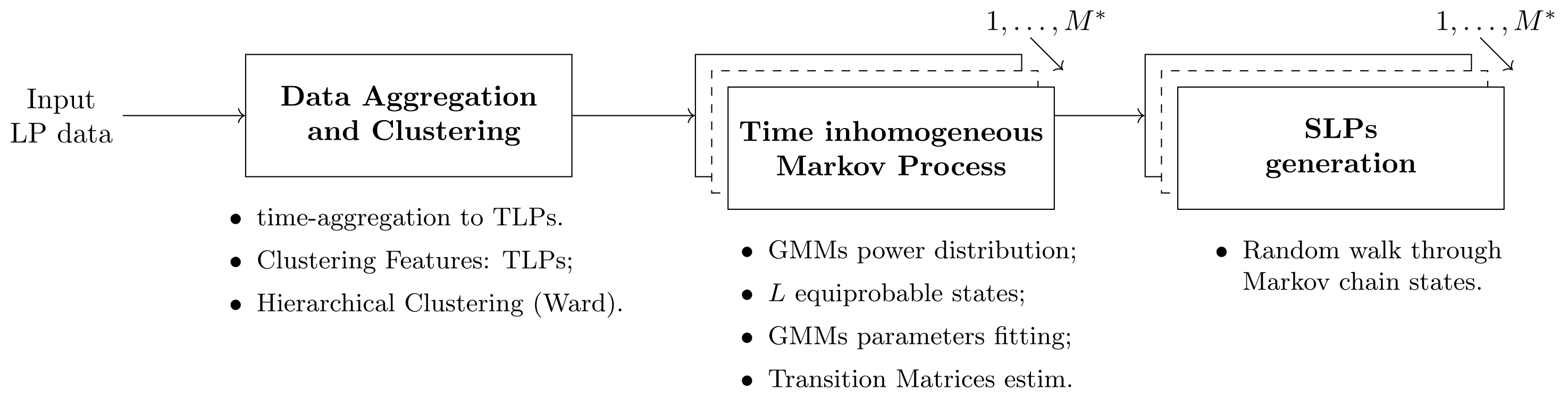
3. Model Description

The model structure is sketched in Figure 1 and consists of three steps:

• data aggregation and clustering,
• Markov chain model definition and
• SLP generation.

In the following, the theoretical background of the steps above is described in detail.

3.1. Data Aggregation and Clustering

Let N be the total number of the yearly load profiles within a given data record. Such profiles have to be clustered on the basis of the similarity of the power consumption patterns of different users. To this end, a preliminary data aggregation step is needed, as also suggested in various other works [29,33,34]. Let T be the number of time steps within a day depending on the sampling period of the available data sets (usually ranging from a few minutes to 1 h). If $p_{nd}\left(t\right)$, for $t=0,\dots ,T-1$, $n=1,\dots ,N$ and $d=1,\dots ,D$, represents the power consumption profile of the $n$-th user in the $d$-th day of a given season of the year, the corresponding TDLP is given by ${\overline{p}}_n\left(t\right)=\frac{1}{D}{\sum }_{d=1}^D{p}_{nd}\left(t\right)$. This average-based data aggregation approach is independent of the time resolution of the data set considered, provided that the time step is the same for all users. Unlike other solutions [29,33,37], neither normalization nor filtering are applied to the load profiles, as recommended in [30,38]. In fact, several normalization techniques were explored, but no noticeable performance improvements were observed.

The TDLPs ${\overline{p}}_n\left(t\right)$ for $n=1,\dots ,N$ are processed by an AHC algorithm [47]. This algorithm groups the input TDLPs into a multilevel binary cluster tree (or dendrogram). The linkage criterion adopted in this paper for grouping is the so-called Ward’s minimum-variance method, which minimizes the within-cluster variance, namely, the sums of squares of the distances between the TDLPs in a cluster and its centroid. This choice is due to the fact that the Ward’s method was already successfully adopted in studies on load profiles modelling and it is recognized as one of the best linkage methods [34], as it prevents the formation of large clusters [29]. Denoting with ${\mathcal{N}}_i$ the set of clusters at the i-th level of the dendrogram, the steps of the AHC algorithm implemented in this work are summarized below.

• Initially, the elements of ${\mathcal{N}}_0$ (i.e., at level 0 for a sequence number $j=0$) are exactly N clusters consisting of 1 TDLP each. As a consequence, the initial NOC value M is $M=|{\mathcal{N}}_0|=N$ and the $M\times M$ dissimilarity matrix $D^j$ is computed as follows:

  $$D^j=\left[\begin{array}{ccccc}0& d_{12}^2& \cdots & d_{1(M-1)}^2& d_{1M}^2\\ d_{21}^2& 0& \cdots & d_{2(M-1)}^2& d_{2M}^2\\ ⋮& ⋮& ⋮& ⋮& ⋮\\ d_{M1}^2& d_{M2}^2& \cdots & d_{M(M-1)}^2& 0\end{array}\right]$$

  (1)

  where $d_{rk}$ is the distance between each pair of clusters r and k. If the Ward’s method is used, initially $d_{rk}$ coincides with the squared Euclidean distance between TDLPs ${\overline{p}}_r\left(t\right)$ and ${\overline{p}}_k\left(t\right)$, i.e., $d_{rk}=\left|\right|{\overline{p}}_r\left(t\right)-{\overline{p}}_k\left(t\right){\left|\right|}_2$.
• Starting from the current matrix $D^j$, the clusters with the least dissimilarity, i.e., those with indexes

  $$(r^{*},k^{*})=arg\underset{r,k\in {\mathcal{N}}_i}{min}{d}_{rk}$$

  (2)

  are merged into a new cluster and the sequence number j is incremented by 1. Furthermore, matrix $D^j$ is updated by deleting the rows and columns associated with clusters $r^{*}$ and $k^{*}$, and by adding a new row and column including the distances $d_{pk}$ between the newly formed cluster (labeled as p) and all the others. In particular, if the Ward’s linkage method is used, the value of $d_{pk}$ is updated recursively using the Lance–Williams expression reported in [48,49]. Observe that both the number of clusters M and the size of matrix $D^j$ are decreased by 1.
• If $M>1$ a new clustering attempt is performed restarting from step 2; otherwise the algorithm ends.

Note that while the leaves of the tree are one-member clusters including the individual TDLPs, the root of the dendogram consists of a single cluster containing the whole data set. Thus, a crucial point is the selection of the best NOC value $M^{*}$, namely, the number of clusters ensuring the best partition of the original data set into subsets of TDLPs with similar features and with minimal error probabilities. While the $M^{*}$ value is usually set a priori [50], in this work $M^{*}$ is unknown. Therefore, it is set heuristically by evaluating the quality of clustering. To this end, several performance indexes exist (most notably the Davies-Bouldin index—DBI [51], the Calinski–Harabasz criterion [38], known also as “variance ratio criterion”, the ratio between the “within-cluster sum of squares” and the “cluster variation” [34]). In the case at hand, the DBI was chosen as it is widely adopted in this kind of applications [29,32,33,34,38]. Of course, if $N_m$ (for $m=1,\dots ,M^{*}$) is the number of TDLPs within the $m$-th cluster of set ${\mathcal{N}}_{M^{*}}$, it results that ${\sum }_{m=1}^{M^{*}}{N}_m=N$.

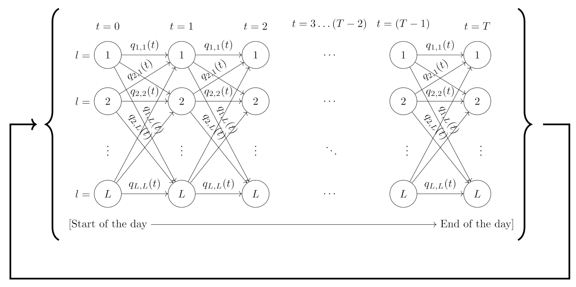
3.2. Markov Chain Model Definition

As known, a Markov chain relies on a given set of states L and on the transition matrices including the probabilities of moving from one state to any other. The rationale underlying the proposed model stems from the observation that even though the PDFs of the power demand of the members of the same cluster changes as a function of time, from the respective cumulative density function CDFs it is always possible to compute the $\frac{1}{L}$-quantiles of the load values at a given time of the day. As a consequence, at every time step a one-to-one correspondence can be established between the states of the model (included in the set $\mathcal{X}=\{X_1,\dots ,X_L\}$) and the probability intervals $[\frac{l-1}{L},\frac{l}{L}]$ for $l=1,\dots ,L$. Quite interestingly, the Markov chain model built as described above exhibits some special properties, i.e.,

• it is irreducible and aperiodic;
• it certainly admits an invariant measure $0\le {\pi }_l\le$ for $l=1,\dots ,L$ with ${\sum }_{l=1}^L{\pi }_l=1$, as the probability of visiting every state $X_1$ of the model is constant over time. In particular, it results by construction that ${\pi }_l=Pr\left\{X_l\right\}=\frac{1}{L}$.
• it is time-inhomogeneous since the elements of transition matrix

  $$Q\left(t\right)=\left[\begin{array}{cccc}{q}_{1,1}\left(t\right)& q_{1,2}\left(t\right)& \cdots & q_{1,L}\left(t\right)\\ q_{2,1}\left(t\right)& q_{2,2}\left(t\right)& \cdots & q_{2,L}\left(t\right)\\ ⋮& ⋮& \ddots & ⋮\\ q_{L,1}\left(t\right)& q_{L,2}\left(t\right)& \cdots & q_{L,L}\left(t\right)\end{array}\right]$$

  (3)
  (with $q_{i,j}\left(t\right)$ being the probability of moving from state i to state j) change as a function of time. Therefore, a sequence of T $L\times L$ transition matrices must be estimated to implement the model.

A graphical overview of the Markov chain is shown in Figure 2. It is important to highlight that properties 2 and 3 at a glance look contradictory. However, they are not, as some examples of time-inhomogeneous Markov chains with a positive probability measure which is invariant in each time step do exist [52]. Recalling that the uniform distribution is an invariant measure for any finite Markov chain with a doubly stochastic transition matrix (i.e., in which not only ${\sum }_{j=1}^L{q}_{i,j}\left(t\right)=1$ for $i=1,\dots ,L$, but also ${\sum }_{i=1}^L{q}_{i,j}\left(t\right)=1$ for $j=1,\dots ,L$), it can be easily shown that in the case at hand this condition holds true by construction. Indeed, the individual transition probabilities in (3) can be estimated from the raw data of the $m$-th cluster as follows, i.e.,

$${\widehat{\pi }}_{i,j}\left(t\right)=\frac{n_{i,j}\left(t\right)}{{\sum }_j{n}_{i,j}\left(t\right)}=\frac{n_{i,j}\left(t\right)}{D·N_m}\forall i,j=1,\dots ,L,t=0,\dots ,T-1,$$

(4)

where $n_{i,j}(t,t-1)$ is the number of transitions between states i and j in the time interval $[t-1,t]$. As the total number of data at each time step within each cluster is constant, not only the elements of the rows, but also those of the columns of (3) sum up to 1, because ${\sum }_{i=1}^L{n}_{i,j}\left(t\right)=D·N_m$. Moreover, the time-inhomogeneous behavior of the considered Markov chain does not affect the invariance property. In fact, recalling that any product of doubly stochastic matrices is also doubly stochastic, the invariant measure $\pi ={[\frac{1}{L},\dots ,\frac{1}{L}]}^T$ certainly satisfies the property $\pi =\pi ·{\mathsf{\Pi }}_{t=0}^{t}Q\left(t\right)$ even in the time-inhomogeneous case, i.e., $\forall t$.

3.3. SLPs Generation

The SLPs associated with a given cluster are generated by a random walk through the states of the Markov chain. Let $p_m\left(t\right)$ (for $m=1,\dots ,M^{*}$) be the random variable modeling the power consumption of the users of the $m$-th cluster at time t, for $t=0,\dots ,T-1$. If $f\left(p_m\left(t\right)\right)$ denotes the PDF of $p_m\left(t\right)$, from the total probability theorem it follows that

$$f\left(p_m\left(t\right)\right)=\sum _{l=1}^{L}f\left(p_m\left(t\right)\right|X_l)Pr\left\{X_l\right\}$$

(5)

where $f\left(p_m\left(t\right)\right|X_l)$ is the conditional PDF of the power consumption in the $l$-th state of the model at time t and $Pr\left\{X_l\right\}={\pi }_l=\frac{1}{L}$ for the reasons explained in Section 3.2. Moreover, recalling that, due to Bayes’ theorem,

$$f\left(p_m\left(t\right)\right|Pr\left\{X_l\right\}))=\frac{Pr\left\{X_l\right|p_m\left(t\right)=p\}·f\left(p_m\left(t\right)\right)}{Pr\left\{X_l\right\}}l=1,\dots ,L$$

(6)

where

$$Pr\left\{X_l\right|p_m\left(t\right)=p\}=\left\{\begin{array}{cc}1\hfill & P_{m,l-1}\left(t\right)\le p<P_{m.l}\left(t\right)\hfill \\ 0\hfill & otherwise\hfill \end{array}\right.$$

(7)

with $P_{m,l-1}\left(t\right)$ and $P_{m.l}\left(t\right)$ being the $\frac{l-1}{L}$-th and $\frac{l}{L}$-th quantiles of the power profile distribution of the $m$-th cluster at time t, it follows that (6) can be rewritten as

$$f\left(p_m\left(t\right)\right|Pr\left\{X_l\right\})=\left\{\begin{array}{cc}L·f\left(p_m\left(t\right)\right)\hfill & P_{m.l-1}\left(t\right)\le p<P_{m.l}\left(t\right)\hfill \\ 0\hfill & \mathrm{otherwise}\hfill \end{array}\right.l=1,\dots ,L.$$

(8)

Therefore, while moving randomly across the Markov chain, the $t$-th sample of the time series representing the SLP of the $m$-th cluster can be generated by triggering one of the L distinct random number generators (depending on the visited state) whose PDF is given by (8).

Of course, in order to apply (8), the expressions of PDFs $f\left(p_m\left(t\right)\right)$ have to be chosen and their parameters have to be estimated by using the very same data that are also used to compute the transition probabilities in (3).

As far as the PDF selection is concerned, the GMMs have been used to keep into account the multi-modal nature of the load distributions for the reasons explained in Section 2.2. In particular, a distinct univariate GMM is used in each time step t, i.e.,

$$f\left(p_m\left(t\right)\right)=\sum _{r=1}^{R_{m,t}}\frac{w_r}{\sqrt{2\pi }{\sigma }_r}{e}^{-\frac{{(p_m\left(t\right)-{\mu }_r)}^2}{2{\sigma }_r^2}}$$

(9)

where:

• $R_{m,t}$ is the number of Gaussian components for the $m$-th cluster at time t;
• coefficients $0<w_r<1$ (for $r=1,\dots ,w_{R_{m,t}}$ with ${\sum }_{r=1}^{R_{m,t}}{w}_r=1$) are the mixing probabilities;
• ${\mu }_r$, for $r=1,\dots ,w_{R_{m,t}}$, are the mean values of the Gaussian components; and, finally, ${\sigma }_r^2$, for $r=1,\dots ,w_{R_{m,t}}$, are the respective variances.

The GMM parameters listed above can be estimated through a standard iterative EM algorithm, as the one described, for instance, in [53]. One key advantage of using a separate univariate GMM for each time step t is that the problem of PDFs parameter estimation can be split into T independent subproblems. Therefore, the total number of parameters to be estimated in each subproblem (as well as their estimation variances and the respective Cramer–Rao lower bounds) tend to be lower than in the multivariate case. Some further details are reported in Section 4.2.

4. Results and Discussion

The model performances have been evaluated both qualitatively and quantitatively by using different test data sets. The use of heterogeneous data sets aims at analyzing the flexibility and trustworthiness of the SLP model in different geographical contexts and with different time steps. This affects the smoothness of the available LPs too, as they typically represent the average power consumption values in every time step.

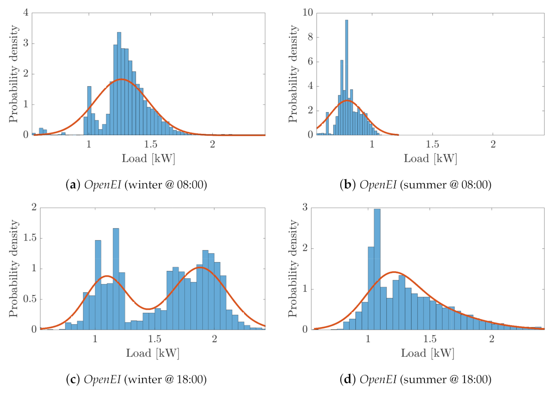
• The first data set, briefly referred to as OpenEI database (OEI – Commercial and Residential Hourly Load Profiles for all TMY3 Locations in the United States, Open Energy Data Initiative, https://data.openei.org/submissions/153 ) includes almost 3000 commercial and residential yearly load profiles reconstructed with hourly resolution on the basis of the weather and location data of the “typical meteorological year 3” (TMY3).
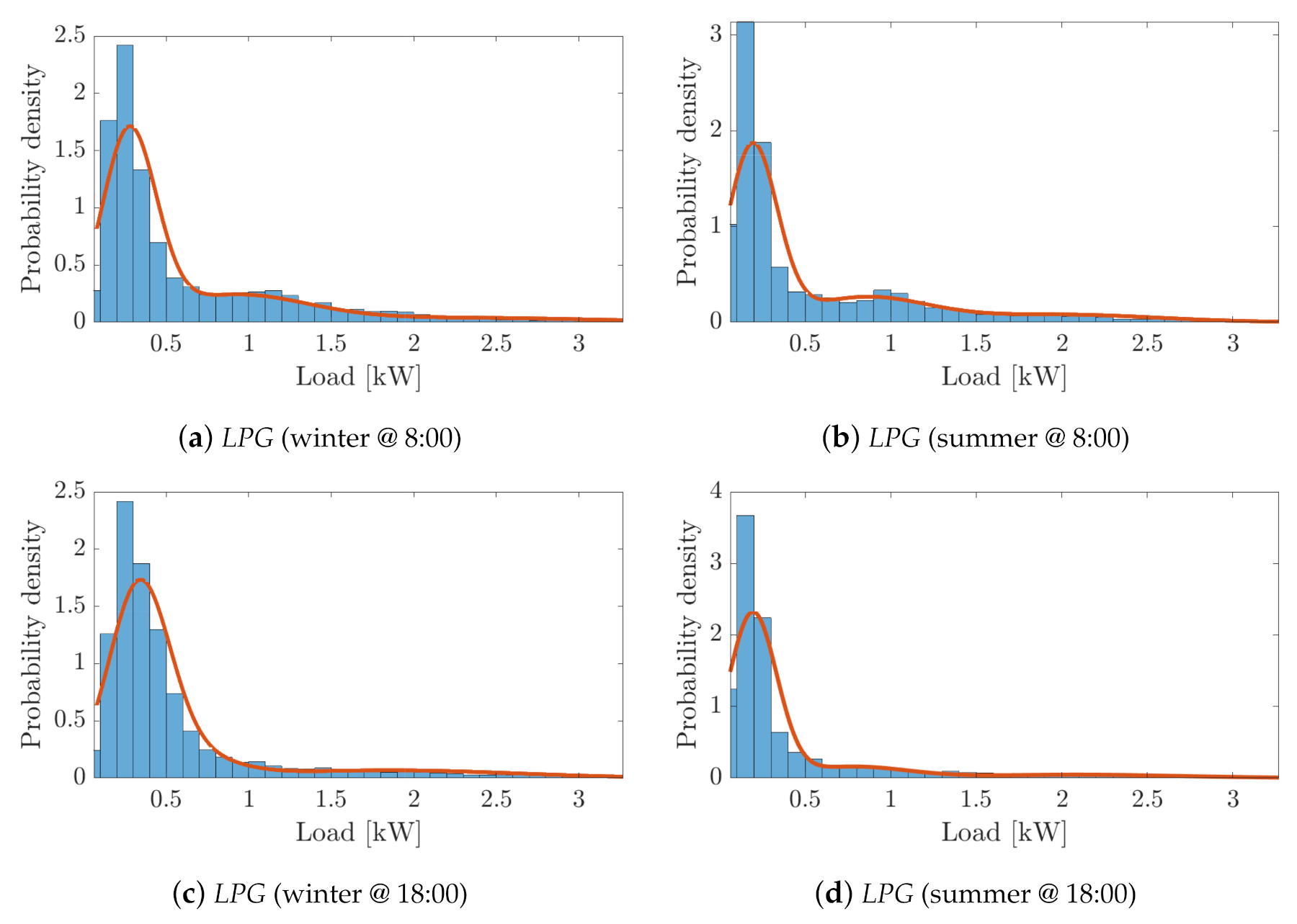
• The second data set, referred to as Load Profile Generator (LPG – A Bottom-Up Customizable Load Generator, Noah Pflugradt, https://www.loadprofilegenerator.de) features around 300 load consumption profiles of typical German households with a 15-minute time step.
• Finally, the third data set, labeled as CER residential (CER Smart Metering Project—Electricity Customer Behaviour Trial, 2009—2010, accessed via the Irish Social Science Data Archive—www.ucd.ie/issda) consists of real anonymized measurement data collected every 30 min from over 5000 Irish households that joined the project.

All records shorter than 1 year or including bad or missing data were excluded from the analysis. Thus, the number of profiles N is equal to 2789 in the OpenEI case, 325 in the LPG case and 3790 in CER residential case. The corresponding values of parameter T are 24, 96 and 48 for OpenEI, LPG and CER residential, respectively.

In the following Subsections, first the clustering results are reported and commented. Then, the criteria to set and estimate the Markov chain parameters are explained. Based on such settings, the statistical performances of the generated SLP are reported. Finally, both a brief discussion about the limitations of the proposed approach and an evaluation of the overall computational burden are provided.

4.1. Clustering Results

As explained in Section 3.1, the AHC algorithm was applied to the N TDLPs of each data set within the same season. Therefore, the clustering results and the Markov chain model parameters change as a function of the season. However, the NOC value of each case study is the the same in all seasons. The choice of computing the mean daily TDLP on a seasonal basis, (i.e., over D days with $D\approx 90$ after splitting each one of the N yearly available LPs into four sub-records, i.e., one per each season) provides a good trade-off between the capability to estimate a typical cluster’s daily pattern and the attempt to account for possible seasonal factors. As explained in Section 3.1, the DBI coefficient was used to compute the best NOC value $M^{*}$. As the DBI results from the arithmetic average of non-negative and symmetric functions of the ratio between the within-cluster scatter and the cluster separation, generally a lower index value means a better clustering. The values of $M^{*}$ associated with the lowest DBI values in each case study are reported in

Table 1. Clustering results obtained with the AHC algorithm applied to the three data set under study, i.e., OpenEI, LPG, CER residential.

Database Name	Population Size N	NOC M	DBI Values	Rejected Clusters	% of Users within Valid Clusters
OpenEI	2789	5	0.61	0	21, 33, 9, 33, 4
LPG	325	7	1.18	1	6, 10, 41, 4, 27, 10
CER residential	3790	5	1.90	0	12, 3, 20, 25, 40

. These numbers are reasonable if compared with those reported in similar studies, e.g., in [30]. In all cases, the clusters including less than $2\%$ of the available LPs were rejected as outliers and no longer used in the following analysis. Table 1 shows also the number of clusters rejected as outliers and the share of customers $\frac{N_m}{N}·100$ (for $m=1,\dots ,M^{*}$) within valid clusters. Observe that, while in most cases the share of customers within a cluster is statistically significant (quite greater than 2%), in a few cases it is borderline. This affects the level of confidence with which the SLPs of those clusters are generated.

4.2. Markov Chains Settings

While the length T of the sequence of transition matrices is dictated by the time resolution of the considered data set, the number of states L of the Markov chain is a degree of freedom. In principle, a high number of states tends to increase the granularity of the model. As a consequence, the SLPs exhibit a finer resolution of the power waveforms. However, incrementing L increases the risk of overfitting problems as well [43]. Moreover, the estimation accuracy of the transition probabilities in (3) and of quantiles $P_{m.l}\left(t\right)$ in (7) decreases, since a larger number of model parameters has to be estimated with the same amount of input data. Last but not least, the computational burden may grow considerably with the number of states L.

Due to the concerns above, we decided to set $L=10$ in all the cases considered in this paper for three reasons:

• this value is small enough (but not too small) to have a reasonably low estimation uncertainty of the elements of transition matrices even with clusters with a low numerosity;
• this number of states is in line with those reported in other works on the same topic, e.g., in [30];
• finally, processing burden and computational times are reasonable, as it will be shown in Section 4.4.

As mentioned in Section 3.2, the elements of the state transition probabilities (3) are estimated through (4) at each time step, whereas the corresponding GMM parameters are computed by iteratively applying the EM algorithm described in [53]. Even though the details of the EM algorithm are out of the scope of this paper, it is worth recalling that the algorithm starts from an initial guess of the number of GMM components $R_{m,t}$ and from a preliminary estimate of the other parameters. In this study, $R_{m,t}$ ranges from 2 to 6, in accordance with the results reported in [31]. For each $R_{m,t}$ value, a preliminary heuristic estimation, rather than a random initialization of the GMM parameters, is performed. In particular, the k-means++ algorithm is used to compute the weight values of each GMM, in order to increase convergence speed. In each iteration, the GMM parameters values are computed through the EM algorithm while maximizing the log-likelihood function. Algorithm convergence is reached when the log-likelihood function does not change significantly from one iteration to the next. To this end, the Bayesian Information Criterion (BIC) is used since the weighting criterion adopted in the definition of this index is particularly effective in penalizing the growing model complexity that, in the case at hand, depends indeed on the number of GMM components. Of course, it is reasonable to select that number of GMM components for which an increment of $R_{m,t}$ does not cause a significant reduction of the BIC value. This good-practice criterion is heuristically implemented through a knee-detection logic [54]. Once the $R_{m,t}$ values are plotted as a function of the BIC ones, this logic identifies the “knee" of the curve, that is the intersection point between the two straight asymptotic lines that best fit the curve. The $y$-axis coordinate of the “knee" point is therefore the value of $R_{m,t}$ to be selected.

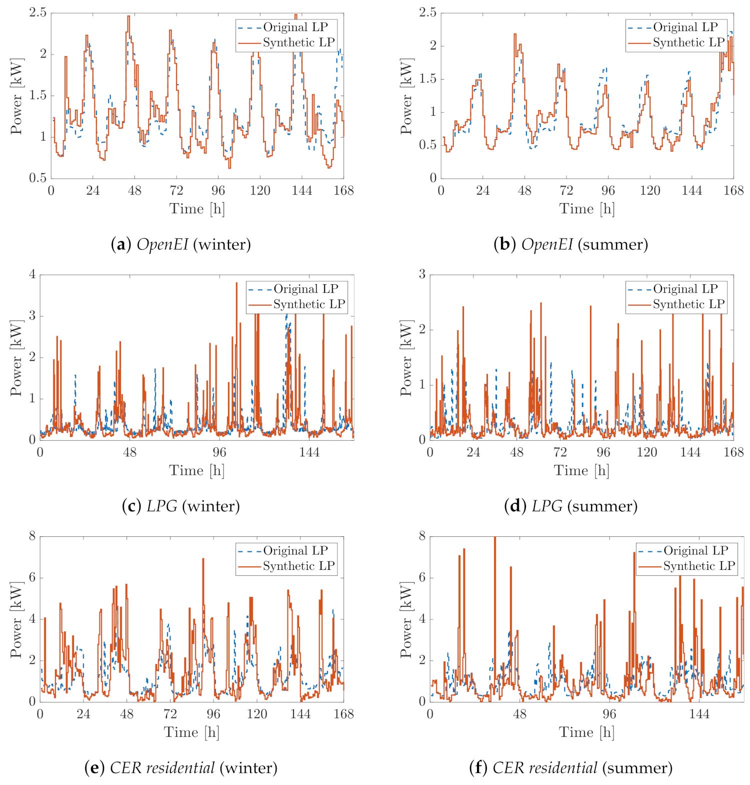
4.3. Performance Evaluation

The evaluation of the model capability to generate SLPs that are statistically similar to the original LPs is performed at three different levels.

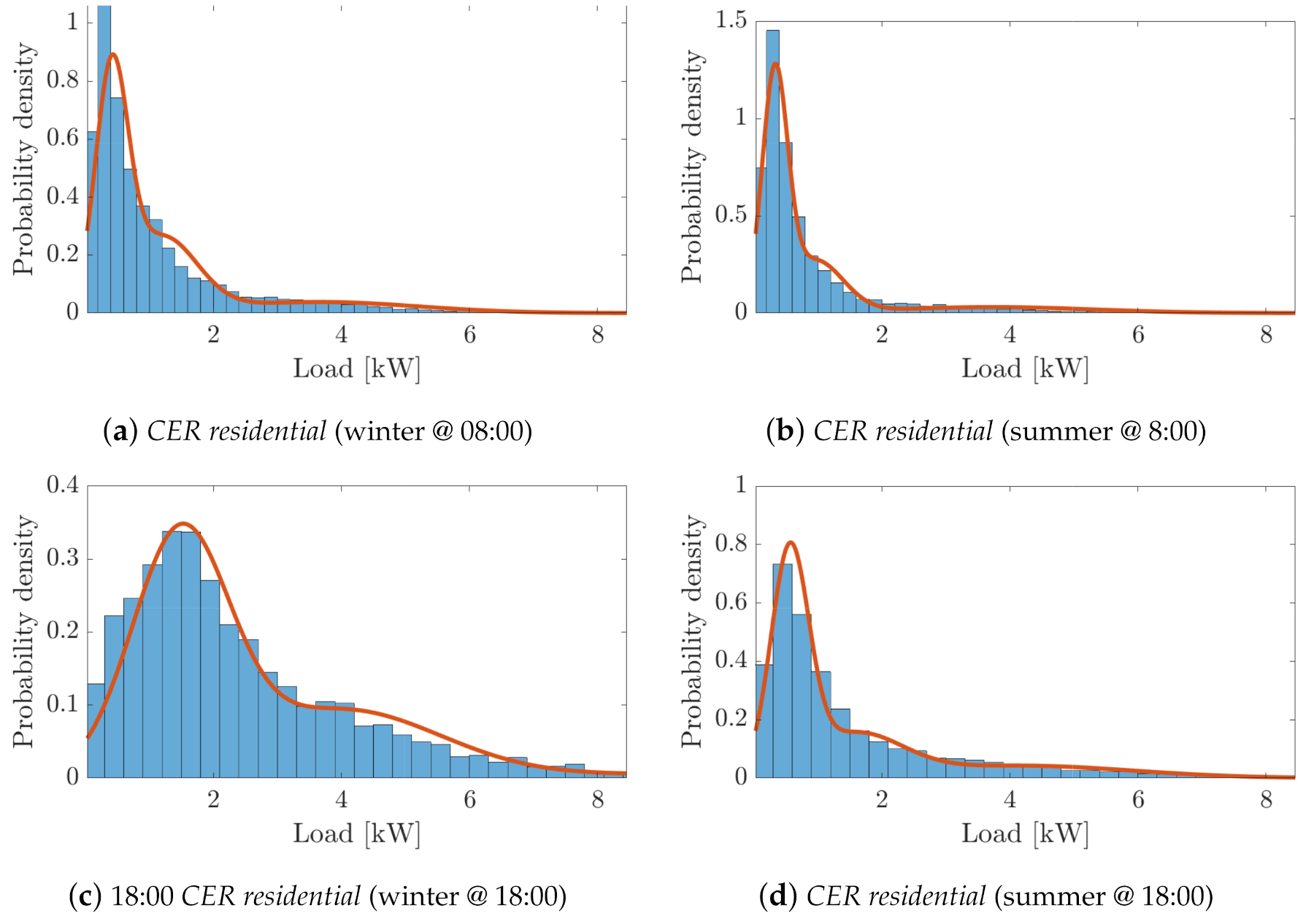
• First, the PDFs of the SLPs are qualitatively compared with the histograms of the original LPs at different times of the day.
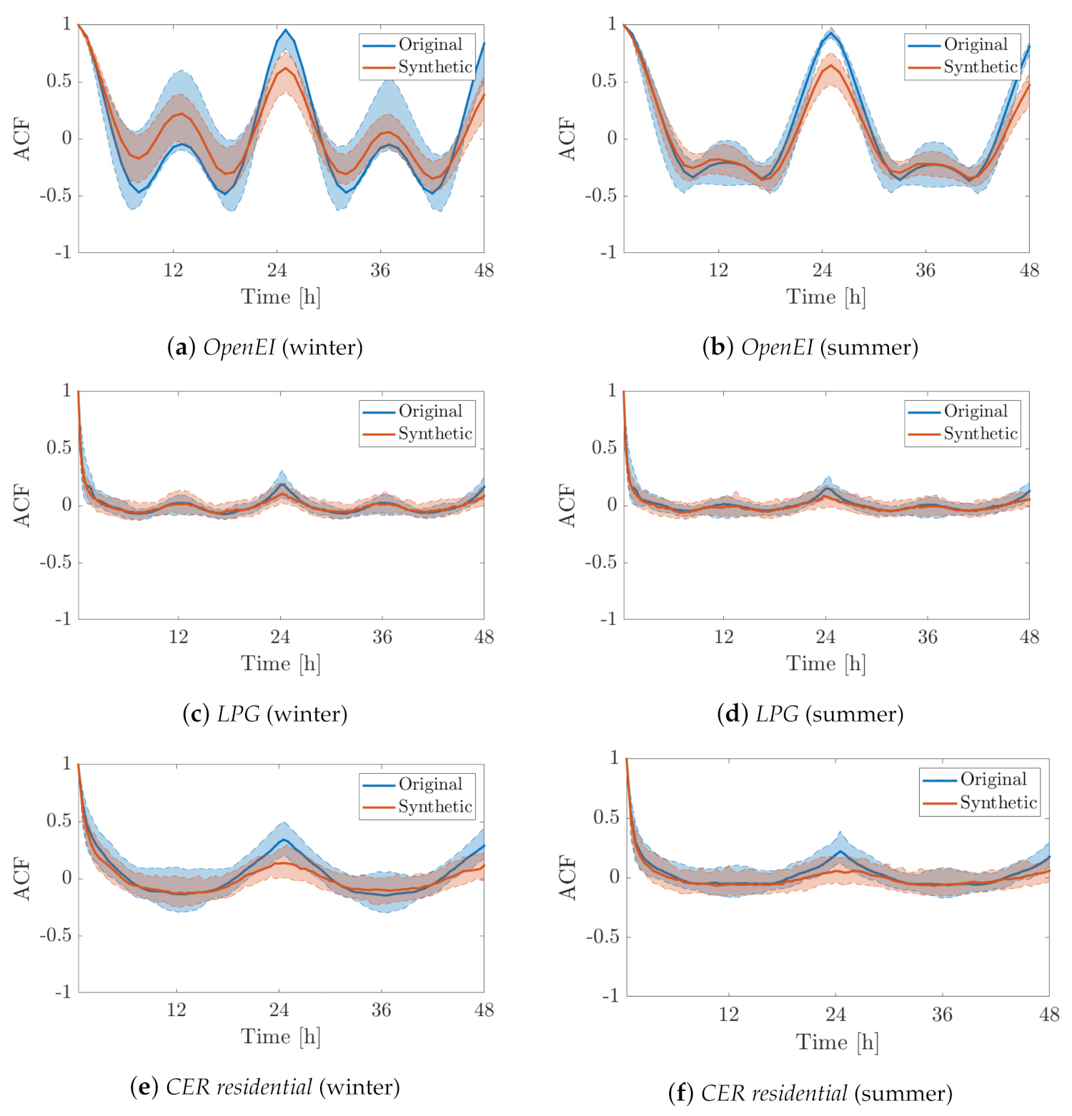
• Then, the capability of the proposed model to describe the intra-day behavior of the original LPs is evaluated by comparing their autocorrelation functions (ACFs).
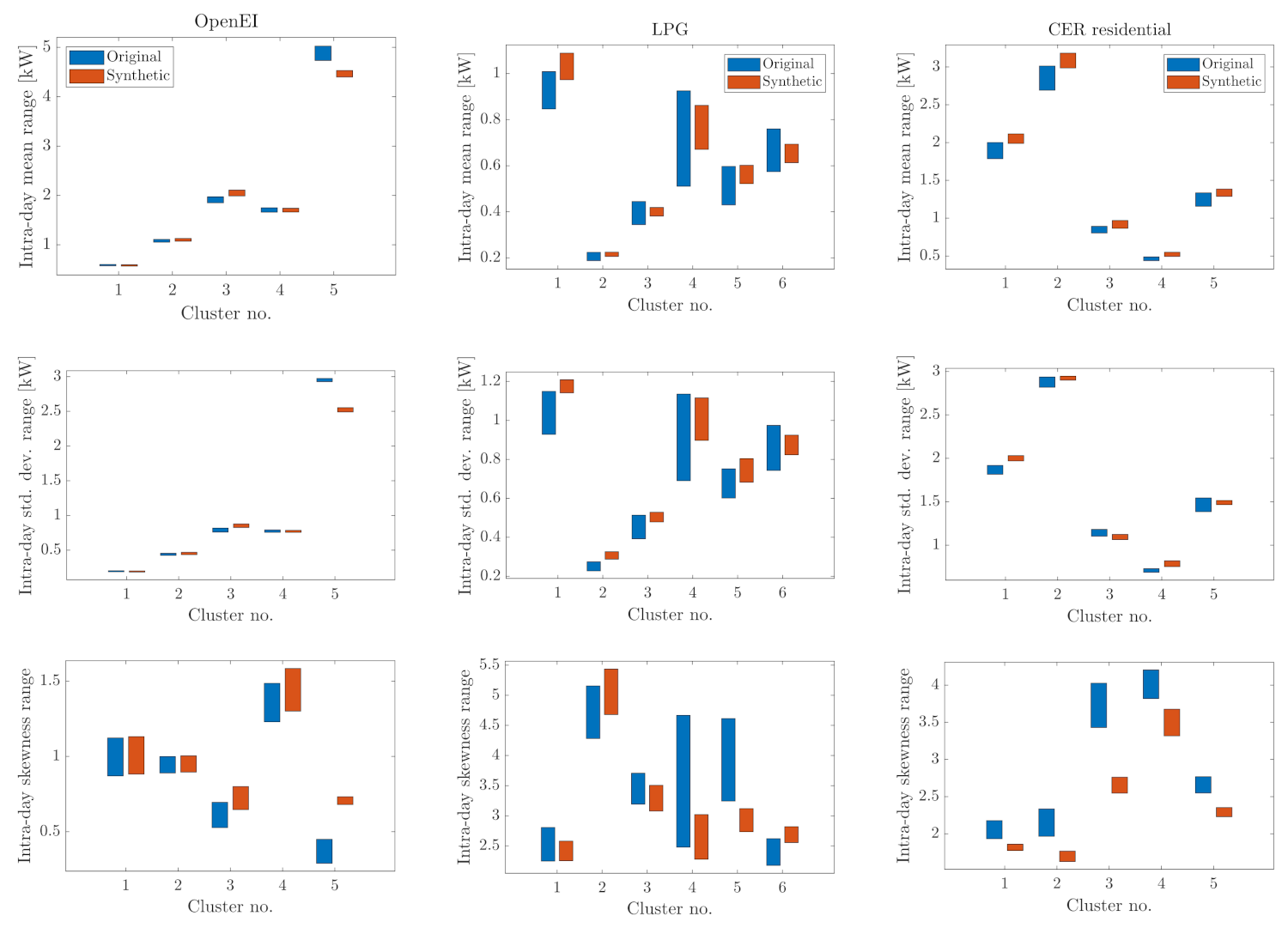
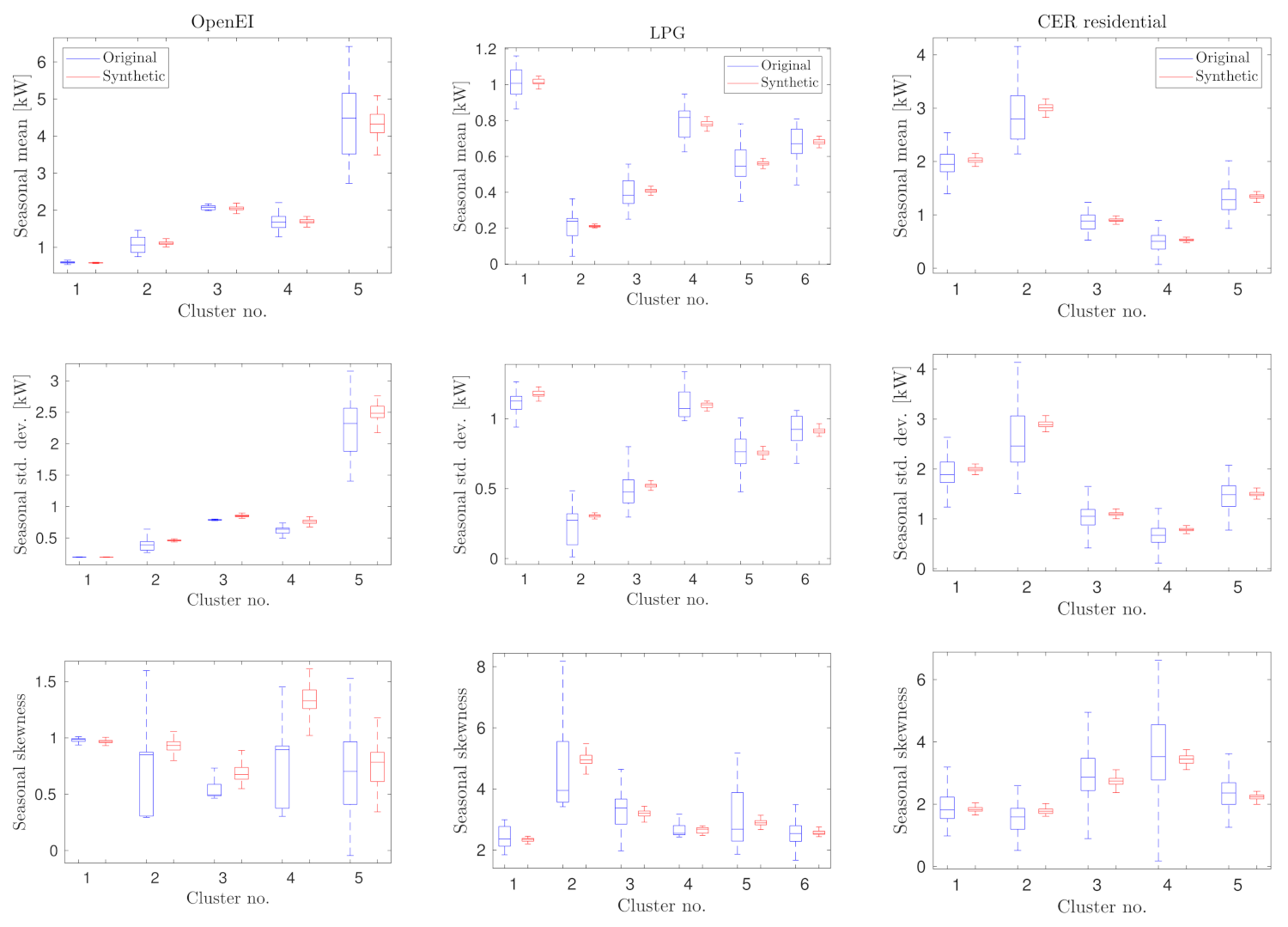
• Finally, a deeper quantitative comparison of the main stochastic features of the load profile distributions is performed. This analysis is carried out for each cluster by comparing the mean, standard deviation and skewness values of the PDFs of both the SLPs and the original LPs, both within a typical day of each season and within the cluster population over the whole season.

Note that any comment or discussion about the specific temporal or stochastic features of the original LPs and the difference between the chosen data sets is out of the scope of this paper. In fact, the purpose of this work is to build a model that is flexible enough to generate SLPs in heterogeneous scenarios, regardless of context-specific aspects.

As far as the similarity of original and synthetic GMM distributions is concerned, the PDFs of the SLPs at given times of the day are compared with the respective histograms of the original LPs. Figure 3a–d, Figure 4a–d and Figure 5a–d show the results of this comparison for the most populated clusters of each data set in the hours when the power consumption is usually particularly high (e.g., at 08:00 and 18:00) in both winter and summer. As the above-mentioned figures show, the proposed model is able to mimic the statistical distribution of the original LPs quite well in all cases, although some sporadic deviations can be observed in the mode values and in the tails of the distributions. Some significant seasonal load variations can be observed in the OpenEI and in the CER case at 18:00. The results in spring and autumn are quite similar and do not provide additional information. Therefore, they are not shown for the sake of brevity. Sometimes, the GMM components are so small or so close that they are not clearly distinguishable in the fitted PDFs of the synthetic data. Nonetheless, the results of Figure 3, Figure 4 and Figure 5 show clearly that the proposed model is flexible enough to reconstruct load distributions with a quite different shape.

In order to assess the capability of the proposed model to track the intra-day variability of the reference data set, the ACFs of original and synthetic load profiles belonging to the same cluster are compared in different seasons. The shaded bands shown in Figure 6a–f represent the intervals between the 0.05-quantile and the 0.95-quantile of the ACF curves within the most populated clusters of each data set in winter and summer, respectively. The quantiles are estimated over 100 original (blue) and synthetic (red) load profiles. The respective median ACFs are also highlighted by thicker lines. Again, the spring and autumn plots are very similar, and therefore they are omitted for the sake of brevity.

The good intra-day consistency of LPs and SLPs is confirmed not only by the evident similarity of the ACFs trend in all cases (regardless of temporal resolution and season), but also by the fact that the ACF inter-quantile band of the ACF curves associated with the SLPs is generally included within the corresponding ACF inter-quantile band of the original profiles. This behavior is quite expected since the original ACFs are computed using pairs of consecutive days over the whole season. Therefore, they may exhibit a larger variability than the ACFs of the synthetic profiles, which instead are based just on the typical (i.e., average) daily behavior of a given season. Further remarks on the limitations of the proposed model over time intervals longer than one day are reported in Section 4.4.

Finally, in order to evaluate and to quantify the differences between the statistical features of the SLPs and the original LPs distributions, about 100 profiles for each cluster of all data sets were extracted in different seasons to build both T separate records of about $100·D$ values each (namely one for every time step) and about 100 dual records of size $T·D$, i.e., one per user over the whole season. The mean, standard deviation and skewness values of such records were then calculated to investigate their statistical behavior and the differences between SLPs and original LPs in two complementary domains, i.e., as a function of time over a typical day (see Figure 7) and within each cluster over the whole season (see Figure 8).

The matrix of bar diagrams in Figure 7 represent the range of mean, standard deviation and skewness (plots in the rows) during a typical winter day for different clusters of different data sets (plots in the columns). The bars in blue refer to the original LPs, while those in red refer to the SLPs. All bars include a number of values equal to the total time steps in a day, i.e., T. Thus, the purpose of Figure 7 is to assess the capability of the model to generate SLPs whose mean value, variability and asymmetry at different times of day are close to those of the original LPs. The daily range of variations of both mean and standard deviation are generally consistent in all cases, although with considerable differences between the data sets. In the OpenEI case, the range values are very small with a negligible offset between the SLP and LP bars in four out of five clusters. The intra-day mean and standard deviation ranges of the clusters of the other data sets are instead larger than in the OpenEI case. Nevertheless, the relative difference between the median of the daily mean values of LPs and SLPs distributions is smaller than 10%, while the median of the respective standard deviations is greater than 10% only for cluster 5 of OpenEI and clusters 1 and 2 of LPG. However, these clusters are among the least populated ones (see Table 1), so the estimated statistical features are inherently affected by larger uncertainty.

The skewness analysis is more controversial. Indeed, the skewness range bars of SLPs and LPs distributions are well aligned and consistent only in the OpenEI case (except for cluster 5 due to its aforementioned larger uncertainty). In the LPG case, the relative offsets between the median values are below 5% on average, but the bars exhibit strong differences from cluster to cluster. In the CER residential case, instead, a dual behavior can be observed, i.e., the skeweness ranges of variations of the SLPs distributions are consistently slightly smaller that those of the original LPs, but they are affected by a strong and well visible negative bias. Such a data set-specific controversial behavior is certainly due to the use of the GMM model, which becomes increasingly critical when the load profiles take on small values for a significant amount of time. This is due to the fact that the domain of synthetic GMM distributions is theoretically unbounded and not just positive. Of course, this is impossible in practice as no negative load values exist in the considered data sets. Even though the negative values that are sporadically returned by the GMM random generators are discarded as outliers, their impact on skewness becomes increasingly relevant as the distribution of the original LPs is mainly concentrated around small positive values.

The matrix of box-and-whiskers plots in Figure 8 show further complementary results, namely, the mean, standard deviation and skewness values (plots in the rows) of both the SLPs and original LPs distributions of up to 100 users for each cluster of different data sets (plots in the columns) over the whole winter season. While Figure 7 aims at evaluating the correctness of the proposed stochastic model within a typical day, the results in Figure 8 are important to assess the statistical consistency of the synthetic profiles within the members of each cluster over a longer time interval.

A first key achievement visible in Figure 8 is that the median values of almost all pairs of boxplots of mean, standard deviation and skewness values are generally well aligned, although those of the original LPs are often slightly overestimated. The absolute relative differences between the median of mean values, standard deviations and skewness of SLPs and LPs distributions are under 7%, 10% and 12%, respectively, in the vast majority of cases. However, in a few sporadic clusters twice as large offsets may occur. Again, the worst results are those about skewness for the same reason explained above.

A second interesting result is that the boxplot range of all the parameters of the SLPs distributions is always much smaller than in the case of the respective original LPs. Therefore, the mean, standard deviation and skeweness values of the LPs distributions of different clusters over the whole season exhibit a much larger variability than those of the respective SLPs distributions. This result was somehow expected since the estimated model parameters refer to a typical day of each season. Thus, possible variability factors occurring within each season are not captured by the model. However, this is not a limitation of the model per se, but it rather depends on the chosen time horizon T considered for both parameter fitting and simulations. Thus, it could be extended if longer data records were available.

The SLPs over one week are still reasonably close to the original LPs. This is indeed visible in Figure 9a–f that shows a qualitative comparison between pairs of randomly extracted one-week-long SLPs and LPs for each data set in winter and in summer, respectively. Figure 9a–f gives an idea of the ability of the model to generate valid SLPs over intervals slightly longer than those used to estimate the model parameters. Clearly, the profiles are reasonably similar, although some differences between SLPs and original LPs can be observed, especially during at the peak consumption times, which are the most complicated to represent with a stochastic model, as already shown in Figure 3, Figure 4 and Figure 5.

4.4. Discussion

The results at the end of Section 4.3 show that, even if the SLPs can potentially have an arbitrary duration, the ability to generate SLPs similar to the original LPs degrades as the length of the output time series grows. As explained above, this is due to the choice of estimating the statistical properties of each cluster from the seasonal TDLPs. This problem could be mitigated by performing both clustering and Markov chain model fitting over observation intervals longer than one day. However, if one-year-long data records are considered, choosing a longer period (e.g., a week) would decrease the number of data available to estimate the typical profiles as well as the Markov chain transition probabilities. This would ultimately affect model parameters estimation accuracy due to need to estimate a larger number of parameters with less data. To partially address this problem, longer data sets (i.e., over multiple years) should be used.

It is likely that an optimal choice of parameters T and D could be made to achieve the best trade-off between simulated time horizon and model accuracy. However, this analysis is very lengthy and it is left for a future work. Nevertheless, even if the intra-week variability is not explicitly considered in the present model, the one-week-long SLPs shown in Figure 9 are generally consistent with the original ones.

Quite importantly, the modeling methodology underlying the synthetic load profile generation is general enough to be applied to the case of active loads as well, i.e., considering prosumers equipped with renewable-based generators that partially reduce the power supply demand from the main grid. This is indeed a further important advantage of a fully stochastic data-driven approach, like the one adopted in this paper. Unfortunately, the available data sets did not allow us to test and to validate the model when active loads are considered.

A final remark concerns the computational burden of the model implementation.

Table 2. Processing times for preliminary data aggregation and clustering, Markov chain parameters estimation and SLP generation. The reported values refer to the steps shown in Figure 1 and are obtained using a PC equipped with an AMD Ryzen™ 5 2600 6C/12T microprocessor, 32 GB of RAM, Linux (Ubuntu 18.04) and Matlab R2019a enhanced with the Parallel Computing Toolbox. The processing times for clustering and model parameters estimation refer to the whole set of clusters for a single season. The SLP generation times refer to one-week-long time series, assuming to generate a number of profiles equal to the number of LPs in the original input data set.

Database Name	Time Resolution	Data Clustering	Model Parameters Estimation	SLPs Generation
OpenEI	1 h	2 min	6 min	3 min
LPG	15 min	52 s	5 min	5 min
CER residential	30 min	15 min	18 min	7 min

reports the total processing times to run the three steps shown in Figure 1 for the three data sets considered in this study. The SLP generation times refer to one-week-long time series in all seasons, assuming that the number of members of each cluster is the same as in the original input data set. Of course, size and time resolution of the original LPs strongly affect the processing times, particularly the GMM parameter estimation due to the iterative EM algorithm. Observe that, in all cases, the SLPs generation times (i.e., step 3) are comparable and they are not excessively high, i.e., in the order of a few minutes. Therefore, once the preliminary clustering and parameters estimation steps are complete, the proposed model is quite scalable, as expected.

5. Conclusions

The capability to generate synthetic load profiles that mimic the power demand of different kinds of users is essential to run realistic and context-specific smart grid simulations. In this paper, a flexible top-down stochastic model is proposed to simulate daily load profiles with features similar to those of a given data set. Some possible target applications of the model are listed below:

• Load flow analyses in time-varying operating conditions, especially when the grid under study consists of many buses and the original LP data are scarce.
• Correct sizing of grid components and devices (e.g., transformers, shunt capacitors and power converters) to improve, at a design level, grid robustness under stressed, non-ideal conditions.
• Definition of possible baseline scenarios to evaluate the impact of different centralized or distributed optimal control strategies for load peak shaving, users’ costs minimization or system resilience improvement.
• Benchmarking of power systems and distribution systems state estimation algorithms.

In order to improve modeling accuracy, the data sets are partitioned on a seasonal basis. Furthermore, a preliminary Ward’s hierarchical clustering is performed to group users whose profiles exhibit a similar average daily pattern. The core of the model is a time-inhomogeneous Markov chain, whose parameters are obtained by fitting a different GMM distribution for each time step. The comparative analysis between the synthetic load profiles obtained through a random walk across the states of the Markov chain in three test cases and the original data sets reveals that the proposed model is able to reconstruct the features of the original profiles quite well in a typical day of each season. Indeed, the autocorrelation functions and the shape of the probability density functions associated with different clusters are very similar. In addition, the median values of the mean and the standard deviation of the synthetic load profile distributions both within the day and within the population of each cluster usually differ by no more than about $\pm 10\%$ from those of the distributions based on the original data. The skewness values are instead not always consistent due to the fact that the load profile distributions are certainly one-sided, whereas the adopted GMM distributions are not. Even if the model was conceived to represent a daily consumption, the model provides reasonably realistic one-week-long synthetic load profiles. However, further research efforts are needed to improve the performance of the model over longer time horizons.

References

1. Ajadi, T.; Cuming, V.; Boyle, R.; Strahan, D.; Kimmel, M.; Michael, L. Global Trends in Renewable Energy Investment 2020. 2020. Available online: https://www.fs-unep-centre.org/wp-content/uploads/2020/06/GTR_2020.pdf (accessed on 3 November 2021).
2. Dharmakeerthi, C.H.; Mithulananthan, N.; Saha, T.K. Overview of the impacts of plug-in electric vehicles on the power grid. In Proceedings of the 2011 IEEE PES Innovative Smart Grid Technologies, Anaheim, CA, USA, 17–19 January 2011; pp. 1–8. [Google Scholar] [CrossRef]
3. Thormann, B.; Kienberger, T. Evaluation of Grid Capacities for Integrating Future E-Mobility and Heat Pumps into Low-Voltage Grids. Energies 2020, 13, 5083. [Google Scholar] [CrossRef]
4. Karimi, M.; Mokhlis, H.; Naidu, K.; Uddin, S.; Bakar, A.H.A. Photovoltaic penetration issues and impacts in distribution network—A review. Renew. Sust. Energy Rev. 2016, 53, 594–605. [Google Scholar] [CrossRef]
5. Pieltain Fernández, L.; Gómez San Román, T.; Cossent, R.; Mateo Domingo, C.; Frías, P. Assessment of the impact of plug-in electric vehicles on distribution networks. IEEE Trans. Power Syst. 2011, 26, 206–213. [Google Scholar] [CrossRef]
6. Macii, D.; Fontanelli, D.; Barchi, G. A Distribution System State Estimator Based on an Extended Kalman Filter Enhanced with a Prior Evaluation of Power Injections at Unmonitored Buses. Energies 2020, 13, 6054. [Google Scholar] [CrossRef]
7. Barchi, G.; Macii, D. A photovoltaics-aided interlaced extended Kalman filter for distribution systems state estimation. Sustain. Energy Grids Netw. 2021, 26, 100438. [Google Scholar] [CrossRef]
8. Wieland, T.; Reiter, M.; Schmautzer, E.; Fickert, L. Modern Grid Planing—A Probabilistic Approach for Low Voltage Networks facing New Challenges. In Proceedings of the 23rd International Conference on Electricity Distribution (CIRED 2015), Lyon, France, 15–18 June 2015; pp. 1–5. [Google Scholar]
9. Ismael, S.M.; Abdel Aleem, S.H.E.; Abdelaziz, A.Y.; Zobaa, A.F. State-of-the-art of hosting capacity in modern power systems with distributed generation. Renew. Energy 2019, 130, 1002–1020. [Google Scholar] [CrossRef]
10. Fatima, S.; Püvi, V.; Arshad, A.; Pourakbari-Kasmaei, M.; Lehtonen, M. Comparison of Economical and Technical Photovoltaic Hosting Capacity Limits in Distribution Networks. Energies 2021, 14, 2405. [Google Scholar] [CrossRef]
11. Alaton, C.; Tounquet, F. Benchmarking Smart Metering Deployment in the EU-28. 2020. Available online: https://op.europa.eu/s/omSNhttps://op.europa.eu/s/omSN (accessed on 3 November 2021).
12. Jardini, J.A.; Tahan, C.M.V.; Gouvea, M.R.; Ahn, S.U.; Figueiredo, F.M. Daily load profiles for residential, commercial and industrial low voltage consumers. IEEE Trans. Power Deliv. 2000, 15, 375–380. [Google Scholar] [CrossRef] [Green Version]
13. Sharma, V.; Haque, M.H.; Aziz, S.M. PV generation and load profile data of net zero energy homes in South Australia. Data Brief 2019, 25, 104235. [Google Scholar] [CrossRef]
14. Machado, J.A.C.; Carvalho, P.M.S.; Ferreira, L.A.F.M. Building Stochastic Non-Stationary Daily Load/Generation Profiles for Distribution Planning Studies. IEEE Trans. Power Syst. 2018, 33, 911–920. [Google Scholar] [CrossRef]
15. Brodén, D.A.; Paridari, K.; Nordström, L. Matlab applications to generate synthetic electricity load profiles of office buildings and detached houses. In Proceedings of the IEEE Innovative Smart Grid Technologies—Asia (ISGT-Asia), Auckland, New Zealand, 4–7 December 2017; pp. 1–6. [Google Scholar] [CrossRef]
16. Bouderraoui, H.; Chami, M. SGSim: Load Profile Generator for Smart Grid Applications. In Proceedings of the 2018 Renewable Energies, Power Systems Green Inclusive Economy (REPS-GIE), Casablanca, Morocco, 23–24 April 2018; pp. 1–6. [Google Scholar] [CrossRef]
17. Uimonen, S.; Lehtonen, M. Simulation of Electric Vehicle Charging Stations Load Profiles in Office Buildings Based on Occupancy Data. Energies 2020, 13, 5700. [Google Scholar] [CrossRef]
18. Corrà, M.; Fusari, E.; Ferrari, A.; MacIi, D. A System Based on IoT Platforms and Occupancy Monitoring for Energy-Efficient HVAC Management. In Proceedings of the 2019 IEEE 5th International forum on Research and Technology for Society and Industry (RTSI), Florence, Italy, 9–12 September 2019; pp. 347–352. [Google Scholar] [CrossRef]
19. Grandjean, A.; Adnot, J.; Binet, G. A review and an analysis of the residential electric load curve models. Renew. Sustain. Energy Rev. 2012, 16, 6539–6565. [Google Scholar] [CrossRef]
20. Richardson, I.; Thomson, M.; Infield, D.; Clifford, C. Domestic electricity use: A high-resolution energy demand model. Energy Build. 2010, 42, 1878–1887. [Google Scholar] [CrossRef] [Green Version]
21. Sandels, C.; Widén, J.; Nordström, L. Forecasting household consumer electricity load profiles with a combined physical and behavioral approach. Appl. Energy 2014, 131, 267–278. [Google Scholar] [CrossRef]
22. Armstrong, M.M.; Swinton, M.C.M.C.; Ribberink, H.; Beausoleil-Morrison, I.; Millette, J. Synthetically derived profiles for representing occupant-driven electric loads in Canadian Housing. J. Build. Perform. Simul. 2009, 2, 15–30. [Google Scholar] [CrossRef] [Green Version]
23. Widén, J.; Wäckelgård, E. A high-resolution stochastic model of domestic activity patterns and electricity demand. Appl. Energy 2010, 87, 1880–1892. [Google Scholar] [CrossRef]
24. Nijhuis, M.; Gibescu, M.; Cobben, J.F.G. Bottom-up Markov Chain Monte Carlo approach for scenario based residential load modelling with publicly available data. Energy Build. 2016, 112, 121–129. [Google Scholar] [CrossRef] [Green Version]
25. Paatero, J.V.; Lund, P.D. A model for generating household electricity load profiles. Int. J. Energy Res. 2006, 30, 273–290. [Google Scholar] [CrossRef] [Green Version]
26. Bottaccioli, L.; Di Cataldo, S.; Acquaviva, A.; Patti, E. Realistic Multi-Scale Modeling of Household Electricity Behaviors. IEEE Access 2019, 7, 2467–2489. [Google Scholar] [CrossRef]
27. Yao, R.; Steemers, K. A method of formulating energy load profile for domestic buildings in the UK. Energy Build. 2005, 37, 663–671. [Google Scholar] [CrossRef]
28. Sandels, C.; Brodén, D.; Widén, J.; Nordström, L.; Andersson, E. Modeling office building consumer load with a combined physical and behavioral approach: Simulation and validation. Appl. Energy 2016, 162, 472–485. [Google Scholar] [CrossRef]
29. Chicco, G.; Napoli, R.; Piglione, F. Comparisons among clustering techniques for electricity customer classification. IEEE Trans. Power Syst. 2006, 21, 933–940. [Google Scholar] [CrossRef]
30. Labeeuw, W.; Deconinck, G. Residential Electrical Load Model Based on Mixture Model Clustering and Markov Models. IEEE Trans. Ind. Inform. 2013, 9, 1561–1569. [Google Scholar] [CrossRef]
31. Singh, R.; Pal, B.C.; Jabr, R.A. Statistical Representation of Distribution System Loads Using Gaussian Mixture Model. IEEE Trans. Power Syst. 2010, 25, 29–37. [Google Scholar] [CrossRef] [Green Version]
32. Räsänen, T.; Voukantsis, D.; Niska, H.; Karatzas, K.; Kolehmainen, M. Data-based method for creating electricity use load profiles using large amount of customer-specific hourly measured electricity use data. Appl. Energy 2010, 87, 3538–3545. [Google Scholar] [CrossRef]
33. Natale, N.; Pilo, F.; Pisano, G.; Troncia, M.; Bignucolo, F.; Coppo, M.; Pesavento, N.; Turri, R. Assessment of typical residential customers load profiles by using clustering techniques. In Proceedings of the 2017 AEIT International Annual Conference, Cagliari, Italy, 20–22 September 2017; pp. 1–6. [Google Scholar] [CrossRef]
34. Tsekouras, G.J.; Hatziargyriou, N.D.; Dialynas, E.N. Two-Stage Pattern Recognition of Load Curves for Classification of Electricity Customers. IEEE Trans. Power Syst. 2007, 22, 1120–1128. [Google Scholar] [CrossRef]
35. Zoltán, K. EU Energy Consumer Classification. Technical Report. Natconsumers Consortium. 2016. Available online: https://ec.europa.eu/research/participants/documents/downloadPublic?documentIds=080166e5aba985df&appId=PPGMS (accessed on 1 November 2021).
36. Benítez, I.; Quijano, A.; Díez, J.L.; Delgado, I. Dynamic clustering segmentation applied to load profiles of energy consumption from Spanish customers. Int. J. Electr. Power Energy Syst. 2014, 55, 437–448. [Google Scholar] [CrossRef]
37. Gerbec, D.; Gasperic, S.; Smon, I.; Gubina, F. Allocation of the load profiles to consumers using probabilistic neural networks. IEEE Trans. Power Syst. 2005, 20, 548–555. [Google Scholar] [CrossRef]
38. Granell, R.; Axon, C.J.; Wallom, D.C.H. Impacts of Raw Data Temporal Resolution Using Selected Clustering Methods on Residential Electricity Load Profiles. IEEE Trans. Power Syst. 2015, 30, 3217–3224. [Google Scholar] [CrossRef] [Green Version]
39. Munkhammar, J.; Rydén, J.; Widén, J. Characterizing probability density distributions for household electricity load profiles from high-resolution electricity use data. Appl. Energy 2014, 135, 382–390. [Google Scholar] [CrossRef]
40. Herman, R.; Kritzinger, J.J. The statistical description of grouped domestic electrical load currents. Electr. Power Syst. Res. 1993, 27, 43–48. [Google Scholar] [CrossRef]
41. Huang, Y.; Zhan, J.; Luo, C.; Wang, L.; Wang, N.; Zheng, D.; Fan, F.; Ren, R. An electricity consumption model for synthesizing scalable electricity load curves. Energy 2019, 169, 674–683. [Google Scholar] [CrossRef]
42. Gros, D.; Wiest, P.; Rudion, K.; Groß, D.; Wiest, P.; Rudion, K. Comparison of stochastic load profile modeling approaches for low voltage residential consumers. In Proceedings of the 2017 IEEE Manchester PowerTech, Manchester, UK, 18–22 June 2017; pp. 1–6. [Google Scholar] [CrossRef]
43. Zufferey, T.; Toffanin, D.; Toprak, D.; Ulbig, A.; Hug, G. Generating Stochastic Residential Load Profiles from Smart Meter Data for an Optimal Power Matching at an Aggregate Level. In Proceedings of the 2018 Power Systems Computation Conference (PSCC), Dublin, Ireland, 11–15 June 2018; pp. 1–7. [Google Scholar] [CrossRef]
44. McLoughlin, F.; Duffy, A.; Conlon, M.; McLoughlin, F.; Conlon, M. The Generation of Domestic Electricity Load Profiles through Markov Chain Modelling. Euro-Asian J. Sustain. Energy Dev. Policy 2010, 3, 12. [Google Scholar]
45. Groß, D.; Wiest, P.; Rudion, K.; Probst, A. Parametrization of stochastic load profile modeling approaches for smart grid simulations. In Proceedings of the 2017 IEEE PES Innovative Smart Grid Technologies Conference Europe (ISGT-Europe), Torino, Italy, 26–29 September 2017; pp. 1–6. [Google Scholar] [CrossRef]
46. Papaefthymiou, G.G.; Klöckl, B.; Klockl, B. MCMC for wind power simulation. IEEE Trans. Energy Convers. 2008, 23, 234–240. [Google Scholar] [CrossRef] [Green Version]
47. Murtagh, F.; Contreras, P. Algorithms for hierarchical clustering: An overview. WIREs Data Min. Knowl. Discov. 2012, 2, 86–97. [Google Scholar] [CrossRef]
48. Lance, G.N.; Williams, W.T. A General Theory of Classificatory Sorting Strategies: 1. Hierarchical Systems. Comput. J. 1967, 9, 373–380. [Google Scholar] [CrossRef] [Green Version]
49. Wishart, D. 256. Note: An Algorithm for Hierarchical Classifications. Biometrics 1969, 25, 165–170. [Google Scholar] [CrossRef]
50. Zhang, T.; Zhang, G.; Lu, J.; Feng, X.; Yang, W. A New Index and Classification Approach for Load Pattern Analysis of Large Electricity Customers. IEEE Trans. Power Syst. 2012, 27, 153–160. [Google Scholar] [CrossRef]
51. Davies, D.L.; Bouldin, D.W. A Cluster Separation Measure. IEEE Trans. Pattern Anal. Mach. Intell. 1979, PAMI-1, 224–227. [Google Scholar] [CrossRef]
52. Saloff-Coste, L.; Zúñiga, J. Convergence of some time inhomogeneous Markov chains via spectral techniques. Stoch. Process. Their Appl. 2007, 117, 961–979. [Google Scholar] [CrossRef] [Green Version]
53. McLachlan, G.; Peel, D. Finite Mixture Models; Wiley Series in Probability and Statistics; John Wiley & Sons, Inc.: Hoboken, NJ, USA, 2000. [Google Scholar] [CrossRef]
54. Salvador, S.; Chan, P. Determining the number of clusters/segments in hierarchical clustering/segmentation algorithms. In Proceedings of the 16th IEEE International Conference on Tools with Artificial Intelligence, Boca Raton, FL, USA, 15–17 November 2004; pp. 576–584. [Google Scholar] [CrossRef] [Green Version]
Figure 1. Block diagram summarizing the main steps of the proposed SLP generation model. The key tasks of each step are also listed.
Energies 15 00269 g001
Figure 2. Representation of the time-inhomogeneous Markov chain for a single cluster. The L states are equiprobable, but the transition probabilities q i , j ( t ) change as a function of the time step t = 1 T . A cyclic random walk throughout the chain is generated to produce SLPs with a duration longer than one day.
Energies 15 00269 g002
Figure 3. Histograms of the OpenEI original LPs and PDFs of the corresponding SLPs (solid lines) at two different times of the day (8:00 and 18:00) in winter and summer, respectively. Histograms computation and GMM PDFs fitting are performed using the same amount of data and refer to the most populated cluster.
Energies 15 00269 g003
Figure 4. Histograms of the LPG original LPs and PDFs of the corresponding SLPs (solid lines) at two different times of the day (8:00 and 18:00) in winter and summer, respectively. Histograms computation and GMM PDFs fitting are performed using the same amount of data and refer to the most populated cluster.
Energies 15 00269 g004
Figure 5. Histograms of the CER residential original LPs and PDFs of the corresponding SLPs (solid lines) at two different times of the day (8:00 and 18:00) in winter and summer, respectively. Histograms computation and GMM PDFs fitting are performed using the same amount of data and refer to the most populated cluster.
Energies 15 00269 g005
Figure 6. Examples of ACF curves associated with the original LPs and the respective SLPs extracted from the most populated clusters of different data set in winter and summer, respectively. The shaded bands comprise the curves between the 0.5-quantile and the 0.95-quantile of 100 original or synthetic ACFs. The median ACFs are also plotted using thicker lines.
Energies 15 00269 g006
Figure 7. Range of variation of the mean, standard deviation and skewness values of the estimated PDFs of the original LPs (in blue) and the corresponding SLPs (in red), respectively, within a typical winter day. Each pair of bars within every plot refers to one of the identified clusters. The columns of the matrix of plots refer to the three explored data sets, while the rows refer to the analyzed statistical features.
Energies 15 00269 g007
Figure 8. Box-and-whiskers plots of the mean, standard deviation and skewness values of the PDFs of the original LPs (in blue) and the corresponding SLPs (in red), respectively, within the population of each cluster over the whole winter season. The columns of the matrix of plots refer to the three explored data sets, while the rows refer to the analyzed statistical features.
Energies 15 00269 g008
Figure 9. Qualitative comparison of one-week-long SLPs and LPs in winter (plots on the left) and in summer (plots on the right). Both the SLPs and the original LPs are randomly extracted from the most populated cluster of each data set.
Energies 15 00269 g009