Methodology for Generating Synthetic Load Profiles for Different Industry Types

Abstract

To achieve its climate goals, the German industry has to undergo a transformation toward renewable energies. To analyze this transformation in energy system models, the industry’s electricity demands have to be provided in a high temporal and sectoral resolution, which, to date, is not the case due to a lack of open-source data. In this paper, a methodology for the generation of synthetic electricity load profiles is described; it was applied to 11 industry types. The modeling was based on the normalized daily load profiles for eight electrical end-use applications. The profiles were then further refined by using the mechanical processes of different branches. Finally, a fluctuation was applied to the profiles as a stochastic attribute. A quantitative RMSE comparison between real and synthetic load profiles showed that the developed method is especially accurate for the representation of loads from three-shift industrial plants. A procedure of how to apply the synthetic load profiles to a regional distribution of the industry sector completes the methodology.

1. Introduction

In 2021, the German government tightened its climate targets; greenhouse gasses were to be reduced by at least 65% by 2030 (55% previously) and at least 88% by 2040, and Germany was to become climate neutral by 2045 (2050 previously) [1]. To achieve these goals, a comprehensive cross-sectoral transformation of the German energy system is necessary. It is generally agreed that greenhouse gas reductions can work only with massive expansions of renewable energy systems [1,2,3,4], with solar and wind energy playing the key roles [5,6,7]. However, decarbonization within the energy economy is not enough. All sectors need to achieve climate neutrality by 2045. In the industrial sector especially, an electrification and thereby coupling with the energy sector is foreseen to be the most economical path to climate neutrality [8,9]. The industry sector consumes more than 40% of the total final energy in Germany, making it the second-largest demand sector after transportation [10]. In terms of electricity, industry even has the highest consumption rate at 45% [11]. As it has already made big contributions toward reducing CO₂ emissions [12], many easy-to-tap efficiency potentials have been exhausted [9]. Nevertheless, apart from sector coupling and the electrification of heat supplies, savings can be achieved through flexibility measures, such as load shifting and demand responses [2].

Future energy systems will be characterized by time-of-day-, weather- and location-dependent renewable-energy supplies. To analyze Germany’s whole energy system for future scenarios, the demand sectors should be provided for energy system models at high resolutions in terms of time, areas and industry sectors for energy system analyses. This is not yet the case in many models.

Most energy system models depict the energy supply sector at a high level of detail [13]. The demand sectors (household, transportation, trade and commerce) are mostly modeled in spatiotemporal resolutions as well [13]. In contrast, the industry sector is often represented in only rudimentary ways [13]. While high-quality load data are potentially available, as most of the industrial consumers are power-metered customers, companies consider their energy consumption data confidential [14], and high spatiotemporal load data are scarce. At the same time, the modeling of industrial energy consumption is showing an increased complexity since consumption tends to show lower dependencies on exogenous influencing factors (e.g., weather) and partly tends to show very weak patterns [13].

This research gap, given the lack of detailed industrial load profiles for energy-system analyses, is to be addressed in this publication with the proposal of a methodology for generating synthetic load profiles for different industry types. The methodology is described, published as an open source as well as evaluated with respect to real available load data.

2. Literature Overview

The numerous energy system models that are currently available use electricity demands quite differently in terms of temporal, spatial and sectoral resolutions [15]. Some energy system models, e.g., Calliope [16], COMPETES [17], EMMA [18], NEMO [19], SAM [20] and Renpass [21], bypass the disaggregation of the different demand sectors by using a total electrical demand [15]. The total cross-sectoral electricity demand can be obtained from the European Network of Transmission System Operators for Electricity (ENTSO-E) [22]. With Urbs [23], a linear-energy system-optimization model, the demand can be separated into commodities, such as electricity, space heat and process heat, but not into the demand sectors industry or households. In HOMER [24], the industrial load is integrated into the primary load along with lights, radio and household appliances, among others. In SWITCH [25], load zones are defined, which can represent either a local area or an electric bus to which one aggregated electrical load is associated, respectively. A number of models prefer to divide the demand into several sectors and integrate the industrial sector separately. Oemof [26] is a Python toolbox for energy-system modeling and optimization, which uses the demandlib library [27] to create load profiles for electricity and heat by using the annual demand. In this library, the industrial electricity demand is modeled by using a step function. The simulation and optimization model REMod-D [28] is used to calculate the transformation of today’s German energy system into a target system in the year 2050. The base electricity load (consumption for original electricity applications) is modeled via load profiles based on data from the ENTSO-E. The electricity demand of the whole industry sector is captured in the base electricity load. PRIMES [29] provides detailed projections of the energy demand, supply, prices and investments that may occur in the future, covering the entire energy system, including emissions for each individual European country and for the European-wide trade of energy commodities. In PRIMES, the industry consists of the ten most energy-intensive branches, split further into 31 sub-branches. Each sub-branch includes a series of industrial processes and energy uses totaling 235 uses. In terms of regional distribution, PRIMES and REMod-D lack spatial information and representation (at a level below that of countries), so they do not fully capture issues about trading infrastructure for fuel and electricity distributions [29]. MyPyPSA-Ger [30] is a model further developed from PyPSA-Eur and has been transformed into a myopic approach. The original PyPSA-Eur [31] model, an open optimization model of the European transmission system, takes the hourly electricity demand profiles for each country from the ENTSO-E [22]. The load time series is distributed to each regional unit by 60% as industrial demand and by 40% as residential demand [31]. With regard to the temporal demand, it is assumed that the top-down load time series shape is the same at each regional node, ignoring local differences and demand sectors. GCAM [32], ReMIND [33], LIBEMOD [34], RETScreen [35] and GENeSYS-MOD v2.0 [36] represent the industrial sector as one aggregated time series as well, while TIMES-D [37], a dynamic intersectoral optimization model, represents the German industrial sector on the basis of 14 predominantly energy-intensive industries, which are modeled as either process- or application-oriented but without further spatial distributions [38].

None of these examples nor, to the best of our knowledge, any other energy system models that deal with the German power system integrate the industrial demand at high spatiotemporal and sectoral resolutions. The lack of data availability in the industry sector is the main obstacle to this goal [14]. A high spatial resolution would mean a NUTS-3 level with regard to spatial disaggregation. A high temporal resolution would mean hourly to 15-min intervals with regard to time steps. With the increase in the fluctuating electricity supply from renewable sources, the time steps of demand series must decrease in energy-system models in order to model the use of storage technologies and demand-side management. Finally, a high sectoral resolution would mean three- or four-digit-level industry types of the common classification systems, such as the NAICS (the North American Industry Classification System) [39], the ISIC (the International Standard Industrial Classification of all economic activities) [40] and the WZ 2008 (the German classification of economic sectors ) [41]. Most projects that analyze the energy balances of industries or generate load profiles remain at the two-digit classification level and do not disaggregate further [13,42,43]. The representation of industrial electricity demands on this level is by nature aggregated over very heterogeneous structures. This most likely leads to rough inferences about economic relationships and consumer behaviors [44]. For a valid econometric demand analysis, it is important to aim for a homogeneous group of consumers. This implies that energy-demand studies should be conducted with the data in industry fields classified into the smallest possible scale. Only a sectoral and spatially resolved energy-demand model makes it possible to answer current questions, such as the need for the expansion and optimization of electricity grids and the technical and economic potential of functional electricity storage systems [45].

The DemandRegio [13] project identified this gap and provides a program code that models temporal, spatial and industry branch-specific electricity and gas demands. Load profiles are generated at hourly intervals. For industry branches, for which no real data are available, a step function on the bases of shift patterns is applied. With this approach, however, there is a risk that since several step profiles are added up to cover a region, an oversized peak can be built up and demand will abruptly increase and fall at certain points in time. A regional breakdown is realized on the basis of fixed energy-demand-determining variables, such as the number of employees per industrial sector. The industry is clustered into 24 branches according to the second hierarchy of the classification system WZ 2008 [41], also called two-digit levels or divisions.

The dsgrid [46] model explores the future energy system of the United States. It models industrial consumption using the IGATE-E program [47]. This is an industrial load generator that uses historical plant-level load data, the Manufacturing Energy Consumption Survey (MECS) [48] and the load shapes from the EPRI load-shape library [49]. This library provides representative hourly load shapes by using five end-use applications (HVAC, lighting, mechanical drive, process heat and other) and various scenarios, e.g., weekday versus weekend and peak season versus off-peak season, for the sectors commercial, residential and industry for 13 different regions in the U.S.

In fact, the DemandRegio project and EPRI load-shape library are the only accessible load generators presenting hourly time patterns for industry types and industrial end-use applications.

This paper aims to bridge the gap between the industrial sector and the need for a resolved electricity demand for power system analyses. Since there are hardly any freely available industrial load data, the following chapters propose how this gap can be closed by means of a methodology for generating industrial synthetic load profiles.

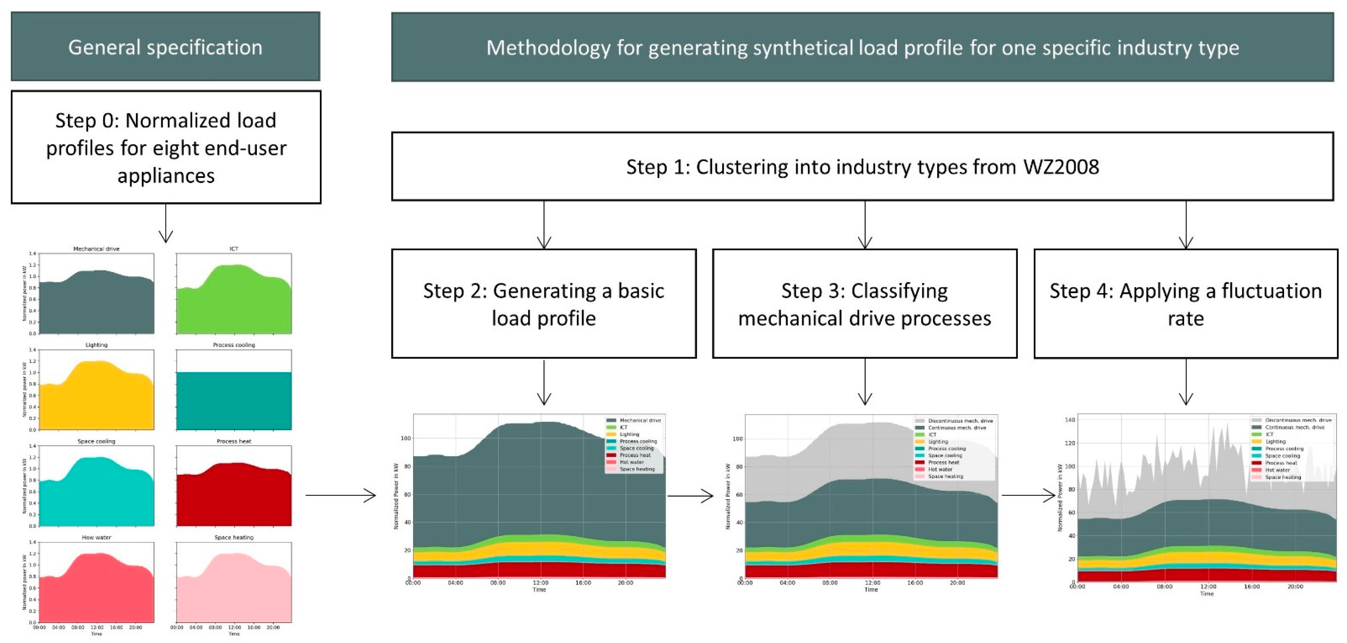
3. Generating Industrial Synthetic Load Profiles

Like the dsgrid project [46], this method was built on the assumption that similar industrial applications have similar electricity demand patterns regardless of the industrial sector in which these applications are used. Based on this assumption, eight electrical end-user categories (e.g., space cooling, lighting and mechanical drive processes) were set, to which daily normalized load profiles were assigned. These eight profiles were the only exogenous data input into the methodology and generated in Step 0. The methodology for generating synthetic load profiles for different industry types was structured into four steps, which were carried out successively. In the first step, certain industry types were specified. In the second step, the electricity consumption of end-use appliances was quantified for each industry type, and basic load profiles were generated top-down. Thereafter, the profiles were further sharpened bottom-up in the third step. There, the typical mechanical drive processes were classified into continuous and discontinuous processes and the load was separated according to their shares. In the fourth step, a synthetic fluctuation was applied to the profile as a stochastic attribute. The individual steps are described in the following chapters and summarized in Figure 1.

Up to this point, the method was limited to the generation of synthetic load profiles for one typical working day since the focus of the method was on the information content and the systematic construction of the load profile.

3.1. Step 0: Normalized Load Profiles for Eight End-Use Appliances

The eight selected end-use categories (referred to in the following sections as end users) are space heating [SH], hot water [HW], process heat [PH], space cooling [SC], process cooling [PC], lighting [L], information and communications technologies [ICT] and mechanical drives [MD] (based on the end-use appliances of the AGEB [5]). Every end-user is assigned to one daily load profile (Figure 2). The EPRI load profiles mechanical drive and process heat show nearly identical patterns and differ by less than 2% of their absolute values [49]. Therefore, the EPRI load profile mechanical drive, for the scenario of an off-peak season, an average weekday (Monday to Friday) and the region Mid-Atlantic Area Council (a similar climate to Germany) was extracted by using the web-based tool WebPlotDigitizer [50]. The resulting time series was recorded in 15-min intervals and normalized to an average consumption of 1. The resulting load profile $x_{\mathrm{Pro}}$ (production) was assigned to the end-users process heat and mechanical drive. The remaining three EPRI load profiles were also almost identical and differed from the first two by stretching in the y direction by a factor of 2. This characteristic was adopted to the second load profile infrastructure,

$$x_{\mathrm{Inf}, i}=2\times x_{\mathrm{Pro}, i}-1$$

(1)

which is generated out of the load profile production, where $x_{\mathrm{Inf}, i}$ is one value of the load profile infrastructure at time i via Equation (1). The whole timeseries $x_{\mathrm{Inf}}$ is normalized to an average consumption of 1 and assigned to the end-users space heating, water heating, space cooling, lighting and ICT. The third load profile constant $x_{\mathrm{Con}}$has a value of 1 at all times.

3.2. Step 1: Clustering into Industry Types

The companies were clustered into industry types according to the systematic classification WZ 2008 of the German Federal Statistical Office [41], which classifies all of the 45,000 German manufacturing companies [51] via five sub-sector levels (

Table 1. Hierarchy of the WZ 2008 classifications [41,51].

Sub-Sectors	WZ 2008 Code	Number of Sub-Sectors in Section C
Sectors	C: Industry (1-digit code)
Divisions	C: 10–33 (2-digit code)	24
Groups	C: 10.x–33.x (3-digit code)	92
Classes	C: 10.xy–33.xy (4-digit code)	187
Sub-classes	C: 10.xy.z–33.xy.z (5-digit code)	260

) by using their end products, their final purposes and their production processes. It claims that for some industries, such as food and machinery, these three criteria correlate quite strongly [41] (p. 20), so it is assumed that companies that have similar products and processes also have similar electricity-demand patterns.

In this paper, industry types out of the divisions (2-digit codes) with the highest numbers of companies in Germany in the year 2019 were defined, which are: food products (WZ 2008 Code: 10 food products) with 4915 companies, metal products (WZ 2008 Code: 25 (metal products)) with 7429 companies and machinery (WZ 2008 Code: 28 (machinery)) with 5485 companies [52]. To select the industry types of the lowest possible levels of sub-sectors, the three divisions were examined regarding the following questions:

• Does the end-product diversity decrease with the branching from divisions to sub-classes?
• Are data available with regard to the end-user electricity demands (for Step 2)?
• Are data available with regard to the machine-drive processes (for Step 3)?
• Does the sub-sector contain more than 100 companies in Germany?

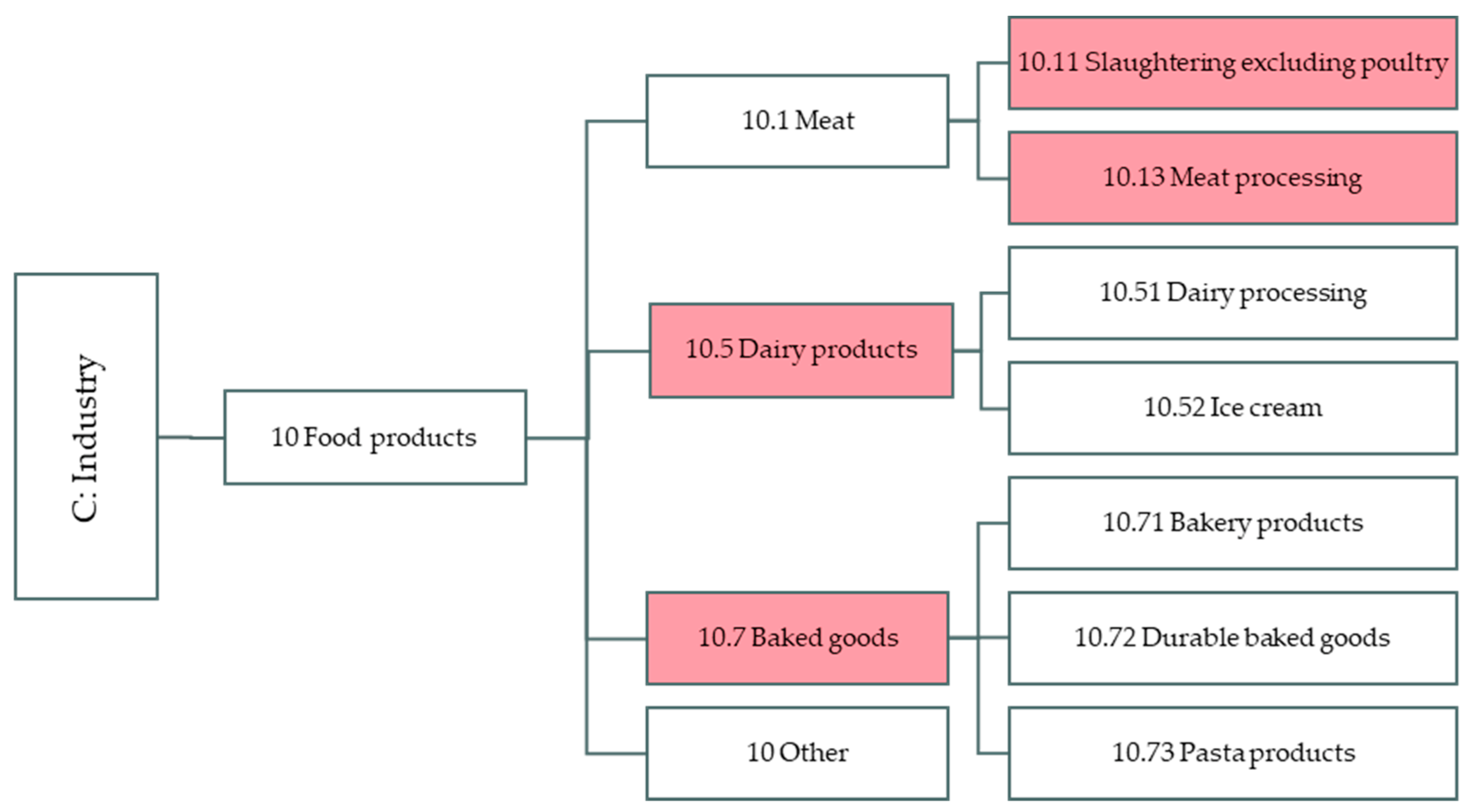
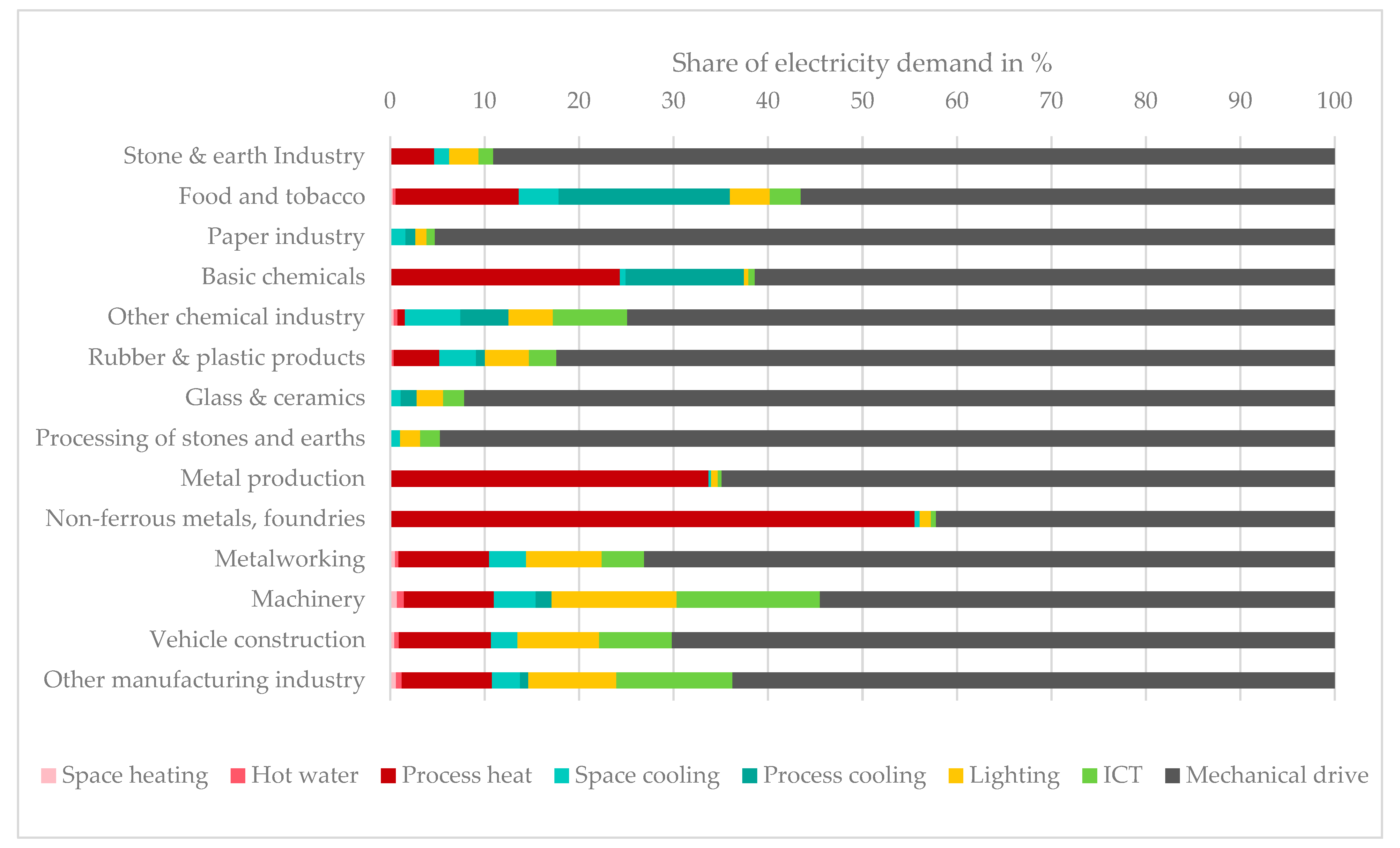
3.2.1. Industry Types of 10 Food Products

The corporate landscape of the food industry is highly heterogeneous (it has a high product diversity) [41], whereas companies at the group or class level (the production of a specific food product) are homogeneous to a high degree [42,53,54,55]. In addition, data availabilities in literature with respect to electricity demands and machine drive processes are relatively high. Therefore, the four industry types highlighted in Figure 3 were selected from the food division. Group 10.5 (dairy products) with 229 companies was separated into only two classes, 10.51 (dairy processing) and 10.52 (ice cream), and as there were only 14 ice cream producing companies in Germany, a further disaggregation was not applied. The companies of 10.71 (bakery products) accounted for 96% of the companies of the higher-level group 10.7 (baked goods), and since the classes 10.72 and 10.73 accounted for fewer than 100 companies [52], 10.7 (baked goods) was defined as one industry type. These four industry types contained 75% of the companies and consumed 48% of the electricity of the food products industry [56].

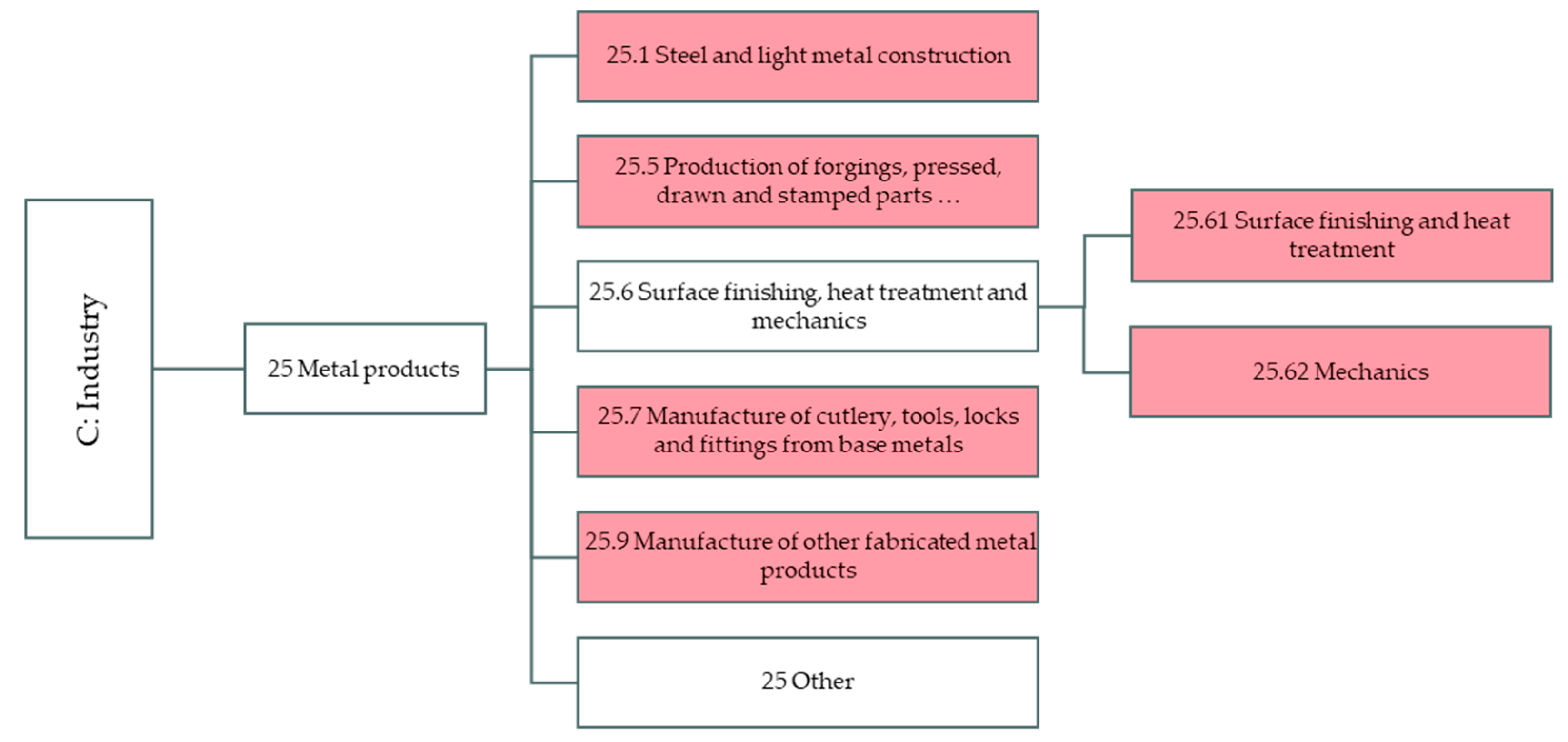
3.2.2. Industry Types of 25 Metal Products

Out of the metal products division, six industry types located at the 3- and 4-digit levels (Figure 4) were selected. They covered 97% of the German metal product companies [51]. Apart from the 2-digit level [57], end-user demands for the metal product industry were hardly published for the lower sub-sectors. Nevertheless, the division was further clustered in this work because, on the one hand, the Austrian Energy Institute of the Economy [58] claimed that “the metalworking companies are a relatively heterogeneous group in terms of their products, their production processes and facilities and their company sizes and structures. However, the companies have (irrespective of their products) similar energy consumptions and key figures, energy source distributions and energy inputs are readily comparable”. Considering this argument, the shares of the end-user electricity of the whole division were applied to each of the chosen industry types in Step 2 (Section 3.3). On the other hand, the data availability for mechanical drive processes is relatively high, and with a consumption of 73% of the electricity [57], it is by far the most important end user.

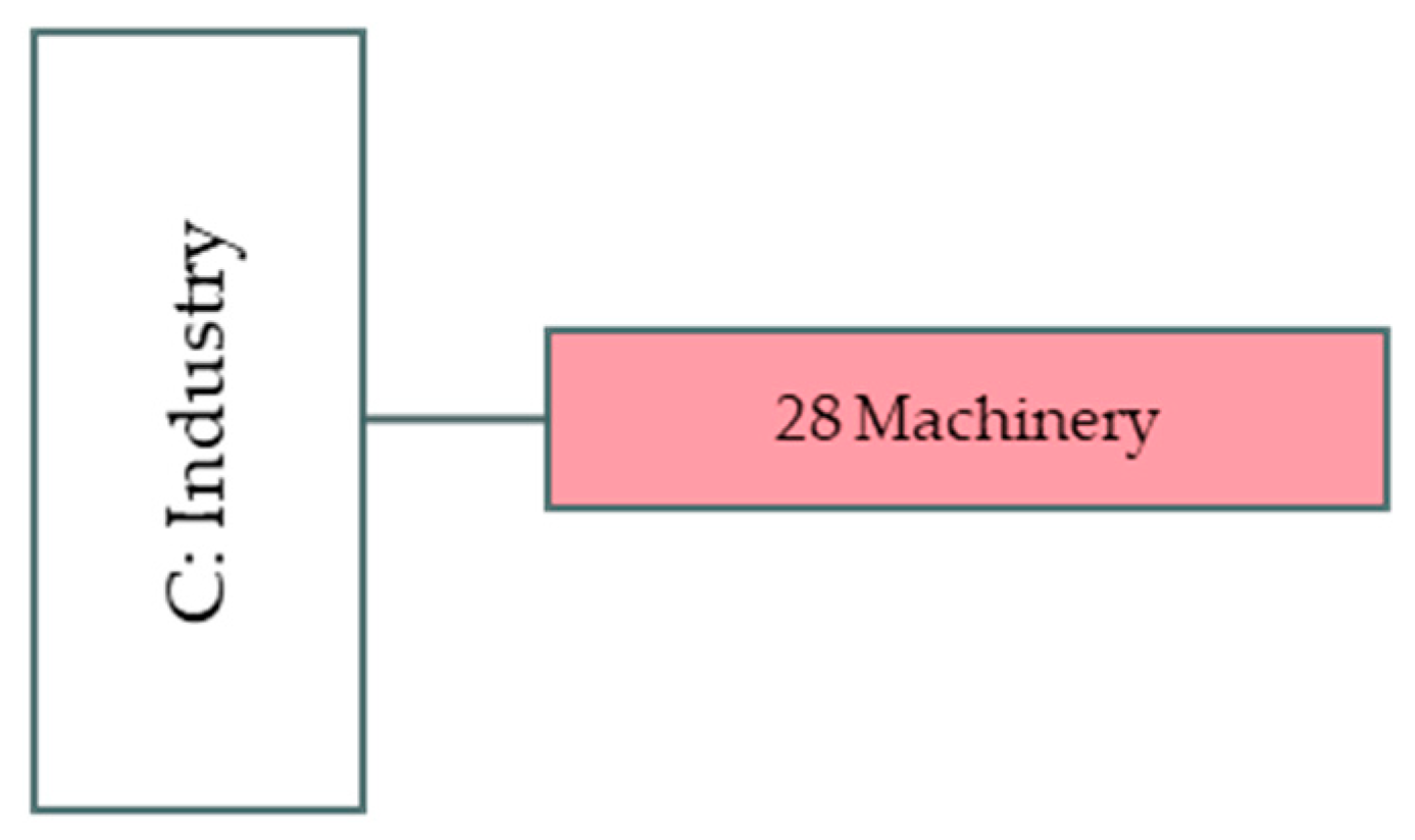
3.2.3. Industry Types of 28 Machineries

For the machinery division, a finer disaggregation will not always result in more uniform industries than for the food and metal products. This is because the product range is broader than that of any other branch of industry [59]. Additionally, a lot of companies in the machinery sector cover only one link of the whole process chain from raw materials to end products. Still, the companies of one chain are classified as one common class [41]. In contrast to the food industry, there are hardly any representative companies in this sector that can be used to map groups or classes. Thus, the machinery division presented itself as a large diverse accumulation of process technologies. In addition, the data landscape for the classes and groups included in this division is very small. For these reasons, the machinery sector was not disaggregated further and the entire division was defined as one industry type (Figure 5).

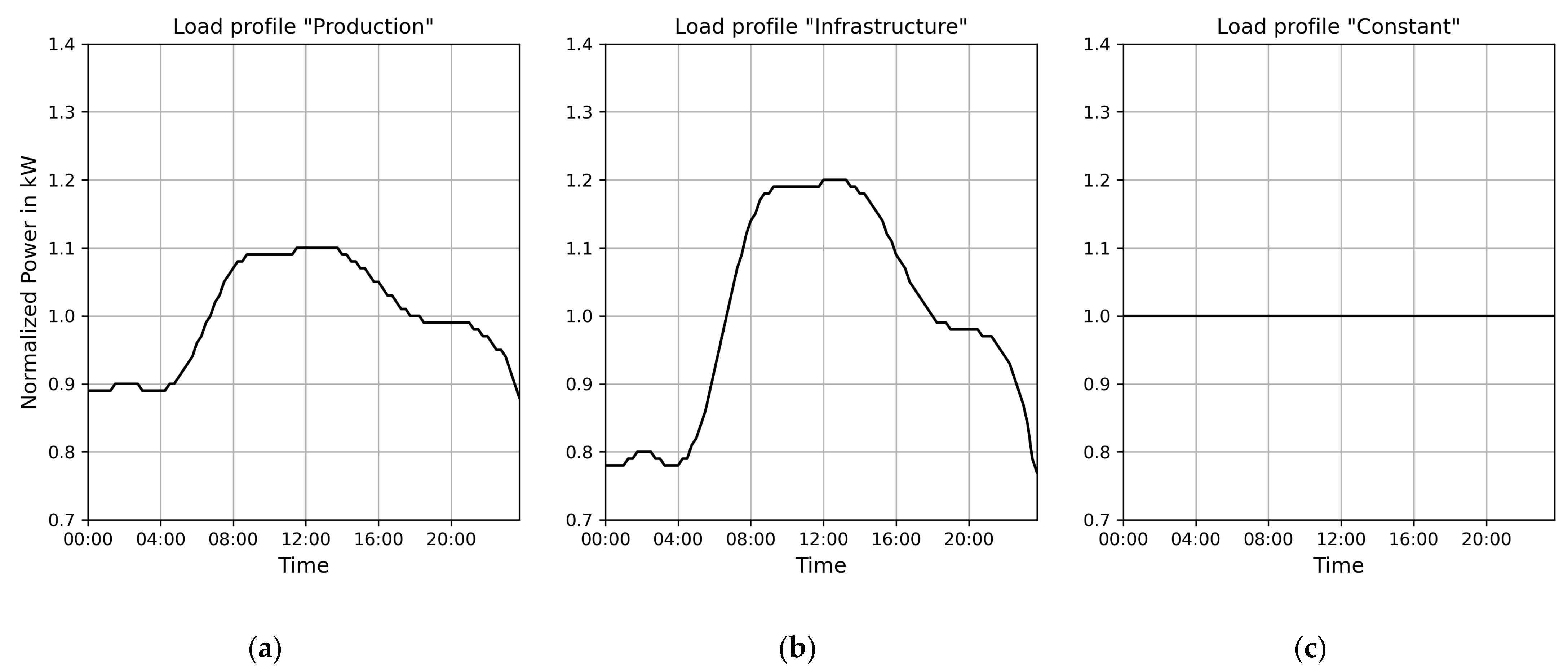
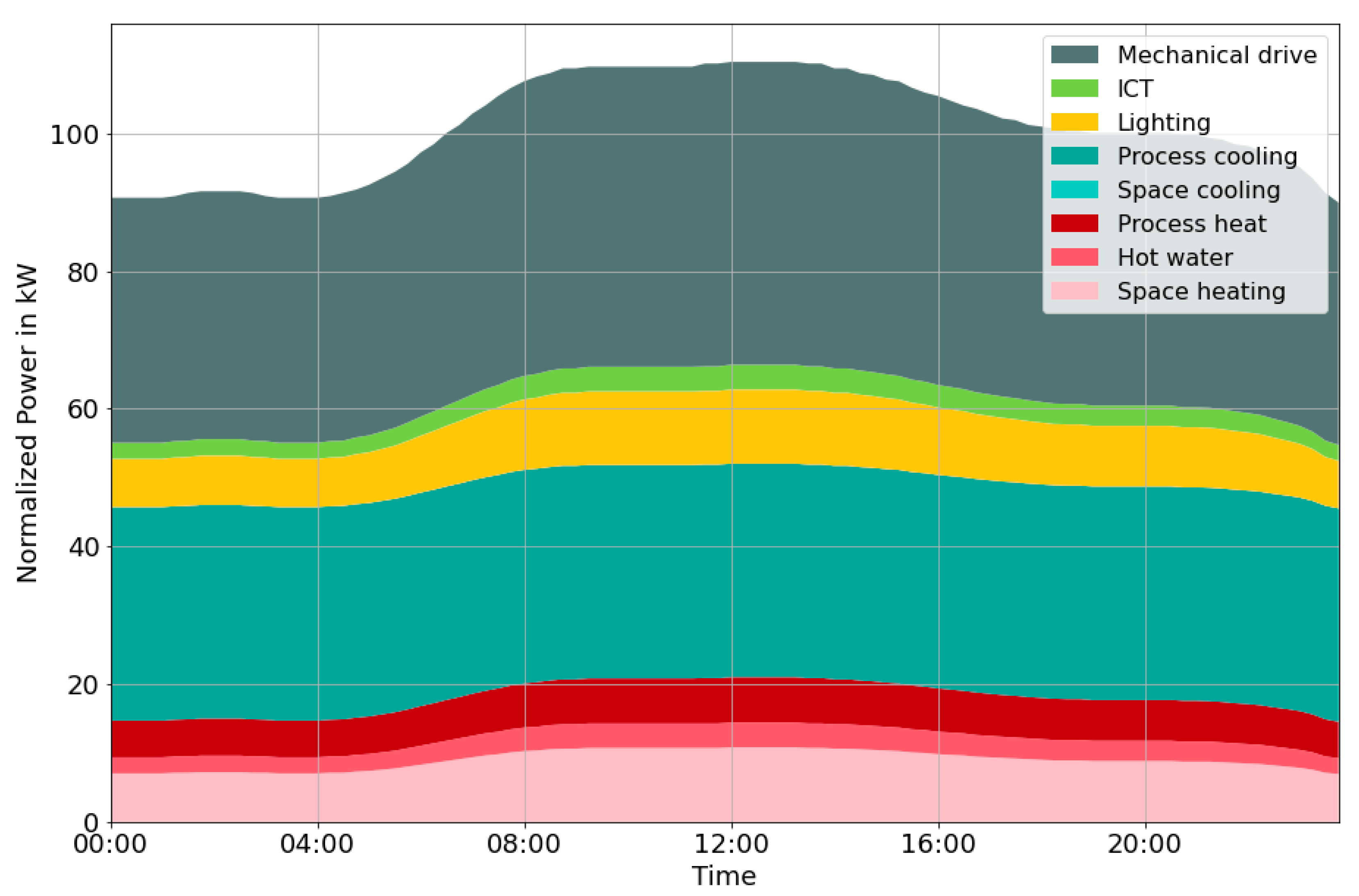
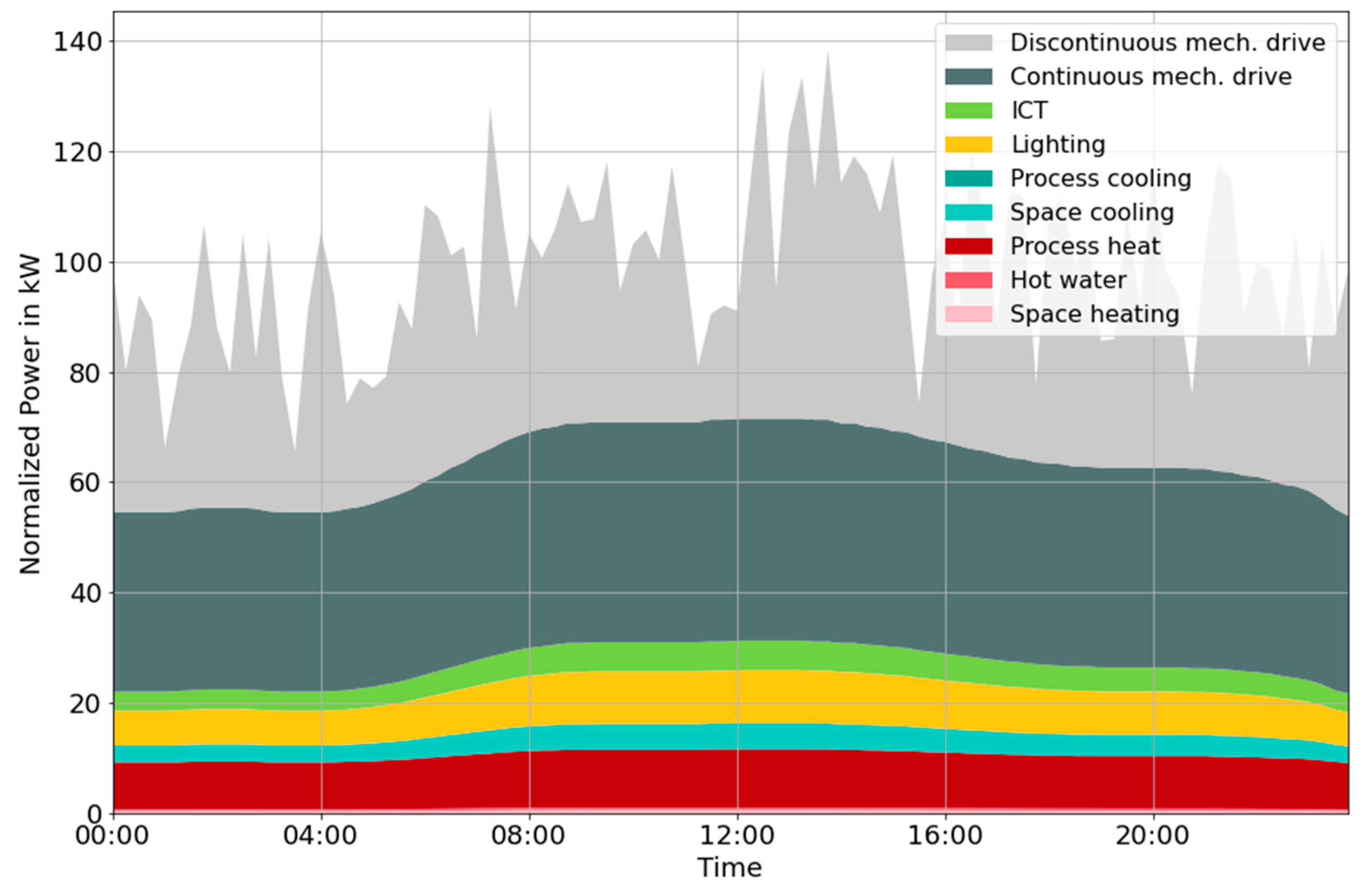
3.3. Step 2: Generating a Basic Load Profile

In this step, the percentage of the electricity demand of the eight end users was first gathered for each industry type.

Table 2. Distribution of yearly electricity demand per end user and industry type.

WZ 2008 Code	Name of Industry Type	Space Heating	Hot Water	Process Heat	Space Cooling	Process Cooling	Lighting	ICT	Mechanical Drives	Source
		p%SH in %	p%HW in %	p%PH in %	p%SC in %	p%PC in %	p%L in %	p%ICT in %	p%MD in %
10.11	Slaughtering, excluding poultry	0.00	0.00	0.00	0.00	51.00	9.00	0.00	40.00	[60]
10.13	Meat processing	6.70 1	0.00	4.80	0.00	39.90	3.90	17.80	26.90	[61]
10.5	Dairy products	9.00 2	3.00	6.00	0.00	31.00	9.00	3.00	40.00	[53]
10.7	Baked goods	2.00 2	0.00	45.00	0.00	30.00	5.00	1.00	17.00	[42]
25.1	Steel and light metal production	0.53	0.36	9.61	3.91	0.00	8.01	4.45	73.13	[57]
25.5	Prod. of forgings, etc.
25.61	Surface finishing and heat treating
25.62	Mechanics
25.7	Manufacturing of cutlery, tools etc.
25.9	Manufacturing of other products
28	Machinery	0.73	0.73	9.54	4.40	1.71	13.20	15.16	54.52	[57]

¹ Ventilation classified as space heating. ² HVAC classified as space heating.

summarizes the collected data. As mentioned in Section 3.2.2, for the six industry types of the metal product industry, the electricity distribution of the division [57] was applied.

For the generation of the basic load profile, each end user’s profile from the first step (Figure 2) was multiplied with the end user’s respective percentage of the total electricity demand p%_{end-user} (Table 2) according to Equations (2)–(9):

$$y_{\mathrm{SH},i}=x_{\mathrm{Inf},i}\ast p{\%}_{\mathrm{SH}}\ast 100\mathrm{kW}$$

(2)

$$y_{\mathrm{HW},i}=x_{\mathrm{Inf},i}\ast p{\%}_{\mathrm{HW}}\ast 100\mathrm{kW}$$

(3)

$$y_{\mathrm{PH},i}=x_{\mathrm{Pro},i}\ast p{\%}_{\mathrm{PH}}\ast 100\mathrm{kW}$$

(4)

$$y_{\mathrm{SC},i}=x_{\mathrm{Inf},i}\ast p{\%}_{\mathrm{SC}}\ast 100\mathrm{kW}$$

(5)

$$y_{\mathrm{PC},i}=x_{\mathrm{Con},i}\ast p{\%}_{\mathrm{PC}}\ast 100\mathrm{kW}$$

(6)

$$y_{\mathrm{L},i}=x_{\mathrm{Inf},i}\ast p{\%}_{\mathrm{L}}\ast 100\mathrm{kW}$$

(7)

$$y_{\mathrm{ICT},i}=x_{\mathrm{Inf},i}\ast p{\%}_{\mathrm{ICT}}\ast 100\mathrm{kW}$$

(8)

$$y_{\mathrm{MD},i}=x_{\mathrm{Pro},i}\ast p{\%}_{\mathrm{MD}}\ast 100\mathrm{kW}$$

(9)

where $y_{\left\{end-user\right\},i}$ is the normalized end-user profile in kW at time point i. Finally, these eight partial loads were summed up to the total load $y_{total}$ as follows:

$$y_{total,i}=y_{\mathrm{SH},i}+y_{\mathrm{HW},i}+y_{\mathrm{PH},i}+y_{\mathrm{SC},i}+y_{\mathrm{PC},i}+y_{\mathrm{L},i}+y_{\mathrm{ICT},i}+y_{\mathrm{MD},i}$$

(10)

The time series of the total load profile was automatically normalized to an average consumption of 100 kW. One exemplary basic load profile for industry type 10.5 (dairy products) is shown in Figure 6.

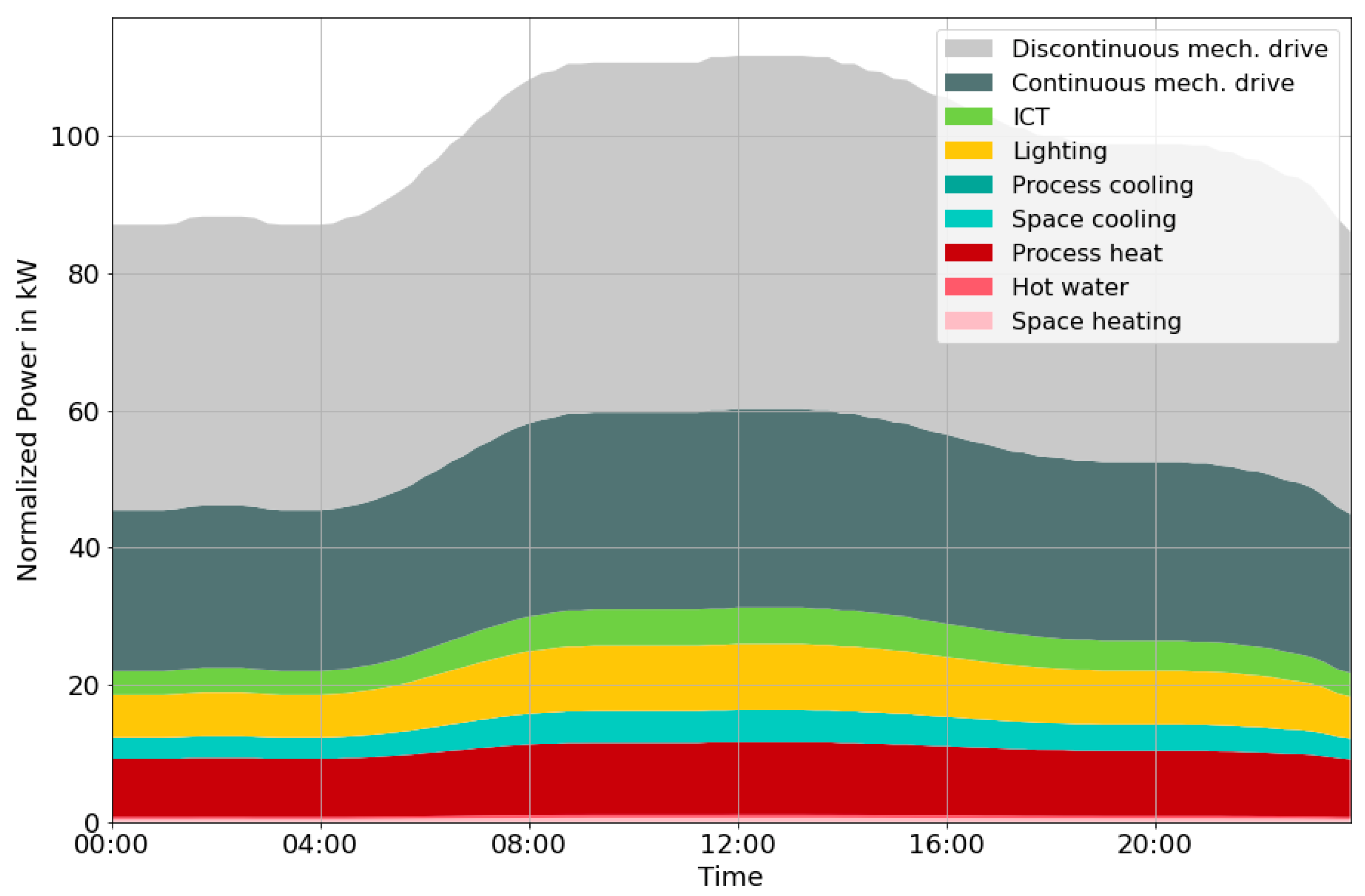
3.4. Step 3: Classifying Mechanical Drive Processes

In the German industry, 72% of the industry’s electricity demand was used for mechanical drive processes in 2019 [57], which made this end user by far the most dominant one. That is why the end user mechanical drive was selected for further characterizations. In this step, for every industry type, the time series of mechanical drive $y_{MD}$ was separated into the two new time series: continuous and discontinuous mechanical drives, i.e., $y_{MD\_conti}$ and $y_{MD\_disconti}$. To calculate the shares of these two categories, the typical mechanical processes of each industry type were classified according to their features listed in

Table 3. Descriptions of the load types continuous and discontinuous mechanical drives based on [43].

	Continuous Mechanical Drives	Discontinuous Mechanical Drives
Description	Manufacturing equipment that applies a constant force to a moving medium, such as a fluid or conveyor.	Manufacturing equipment that applies an abruptly changing mechanical force or electrical charge to a raw material during a defined cycle time.
Machine examples	Mechanical drives, such as pumps, fans, blowers and air compressors.	Mechanical and hydraulic presses, forging presses, grinding machines, chipping machines, etc.
Process examples	Cooling, dewatering pressing, compressing, mixing, final assembly, etc.	Packing, winding, weaving, sawing, planning, chipping, grinding, milling, crushing, classifying, metal cutting, etc.
Power-demand shape	Constant	Fluctuating
DSM potential	Can be modulated	Can be turned on/off

, and their individual power consumptions were quantified (

Table 4. Mechanical-drive [MD] processes of the industry types classified into continuous and discontinuous processes and their shares of electricity demands from the end-user mechanical drives and from the total demand. The dominant process of each industry type is underlined.

WZ 2008 Code	Name of Industry Type	Continuous Processes	Power Consumption	Discontinuous Processes	Power Consumption	Source
			p%MD_conti in %		p%MD_disconti in %
10.11	Slaughtering, excluding poultry	Pumping Air compressing	37.5 12.5	Processing Packaging Conveying	25 12.5 12.5	[62]
	Share of MD demand		50		50
	Share of total demand		20		20
10.13	Meat processing	Air compressing	25	Packaging Filling Cutting Conveying	57 8 8 3	[61]
	Share of MD demand		25		75
	Share of total demand		7		20
10.5	Dairy products	Pumping Mixing Homogenizing Air compressing	22 25 17 22	Packaging Separating	3 11	[64]
	Share of MD demand		86		14
	Share of total demand		34		6
10.7	Baked goods	Pumping Air compressing	42 16	Mechanically treating	42	[63]
	Share of MD demand		58		42
	Share of total demand		10		7
25.1	Steel and light metal construction	Surface cleaning Straightening, bending and rolling Finishing	12 12 12	Cutting Fitting and reaming Fastening	40 12 12	[66]
	Share of MD demand		36		64
	Share of total demand		26		47
25.5	Production of forgings, pressed, drawn and stamped parts …	Shot blasting	15	Cutting Forging Machining Packaging	15 40 15 15	[67]
	Share of MD demand		15		85
	Share of total demand		11		62
25.61	Surface finishing and heat treating	Assembling Cleaning Mixing Coating Drying	10 10 10 40 10	Unpacking Packaging	10 10	[68]
	Share of MD demand		80		20
	Share of total demand		59		15
25.62	Mechanics	Air compressing	50	Cleaning Grinding Milling Cutting Turning	35 2 5 4 3	Own calcu-lations
	Share of MD demand		50		50
	Share of total demand		37		37
25.7	Manufacturing of tools	Rolling Polishing	15 15	Blanking Cutting Forming	15 15 40	[69]
	Share of MD demand		30		70
	Share of total demand		22		51
25.9	Manufacturing of other fabricated metal products	Thread rolling Coating Finishing	9 9 9	Casting Forging Facing Rooving Grinding	9 9 9 9 40	[70]
	Share of MD demand		26		74
	Share of total demand		19		54
28	Machinery	-		-

).

The categorization was done for two reasons. First, continuous and discontinuous processes deliver different types of demand-side management (DSM) products, e.g., regulation, flexibility, contingency, energy and capacity [43]. Second, a fluctuation factor was applied to the proportion of the discontinuous load in Step 4 of this method as this load represents the power consumption of devices with abruptly changing mechanical forces and is therefore mainly responsible for the fluctuating characteristics of load profiles.

The electricity demand of typical processes in food companies is addressed in several publications, such as energy consumption guides [61,62,63] and audits [64]. The processes and their electricity consumptions are listed in Table 4. The processes are also weighted in terms of their power consumptions, their shares of continuous and discontinuous processes related to mechanical drives and to the total demand. For industry type 25.62 (mechanics), we had access to the electricity meters of all machines in the production hall of one company. The mechanical drive devices were first categorized according to their main processes, and the electricity consumption (of the year 2019) of each process was determined. The production processes of the five remaining industry types from 25 metal products were relatively transparent, but there were hardly any data published regarding their electricity consumptions. In this case, assumptions had to be made on one’s own. From the preceding industrial types, it was found that that there was mostly one dominant process (underlined for each industry type in Table 4), consuming between 25% (mixing for 10.5 (dairy products)) and 57% (packaging for 10.13 (meat processing)) of the total electricity for mechanical drive processes. On average, the dominant process consumed approx. 40% of the electricity for mechanical drive applications. For this purpose, one process was defined as the main process to which 40% of the electricity consumption was allocated. The remaining 60% was distributed evenly among the remaining processes. For 28 (machinery), process analysis was complicated because of the heterogeneous consumption structures [12] and a lack of statistical records [65]. That is why Step 3 was skipped for this industry type and Step 4 was followed.

The load mechanical drive $y_{MD}$ was replaced by the two new loads, continuous mechanical drive,

$$y_{MD\_conti, i}=y_{MD,i}\ast p{\%}_{MD\_conti}$$

(11)

and discontinuous mechanical drive,

$$y_{MD\_disconti, i}=y_{MD,i}\ast p{\%}_{MD\_disconti}$$

(12)

where $p{\%}_{MD\_conti}$and $p{\%}_{MD\_disconti}$ are the shares of continuous and discontinuous mechanical processes (Table 4) and add up to 100%. One exemplary result for industry type 25.1 (steel and light metal construction) after the third step is shown in Figure 7.

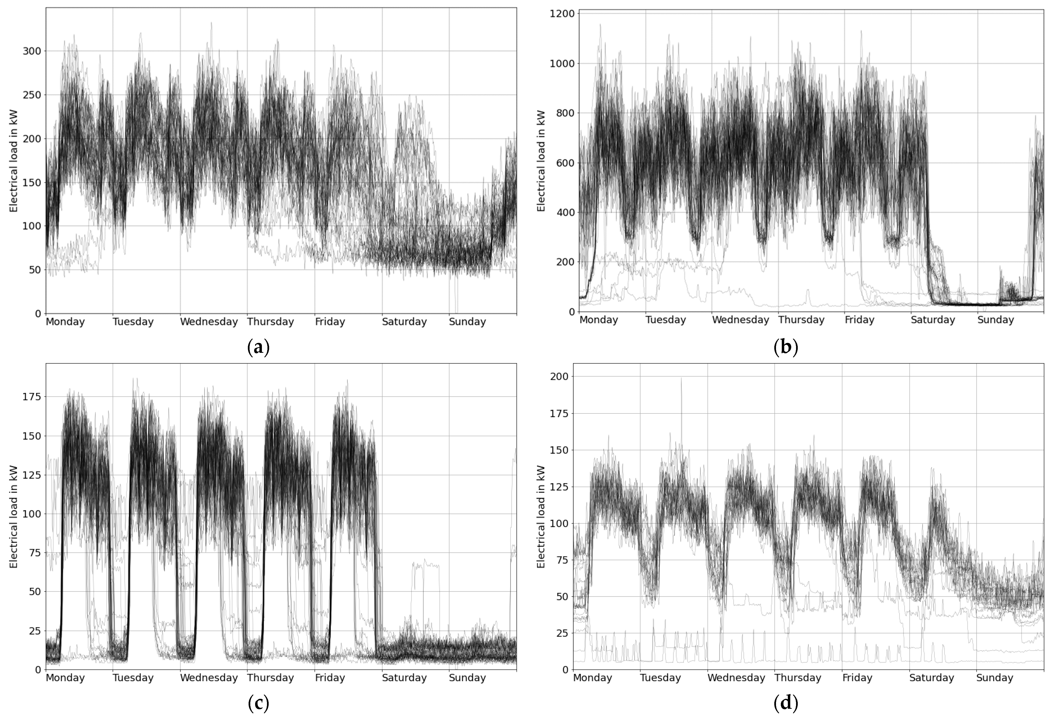
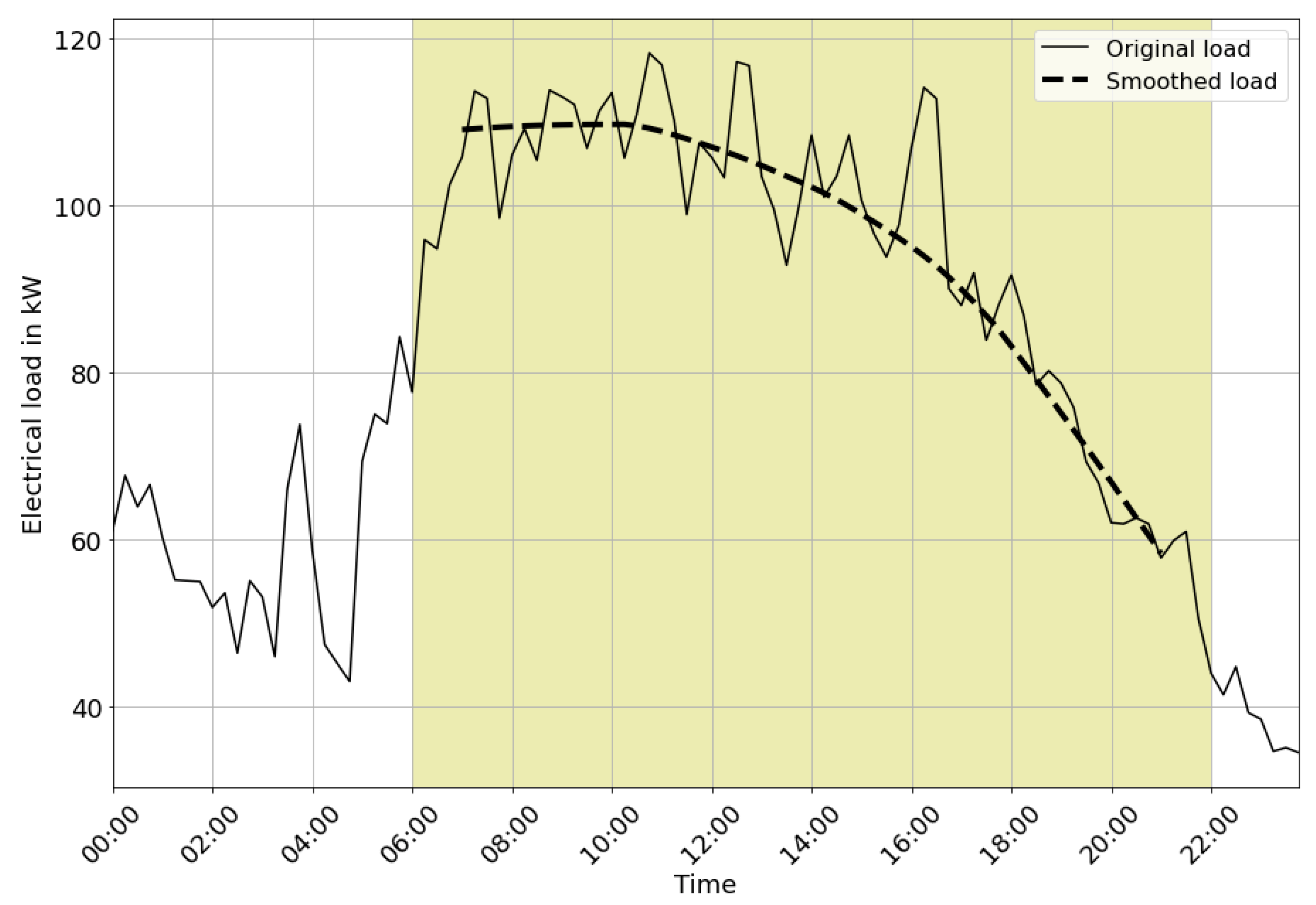
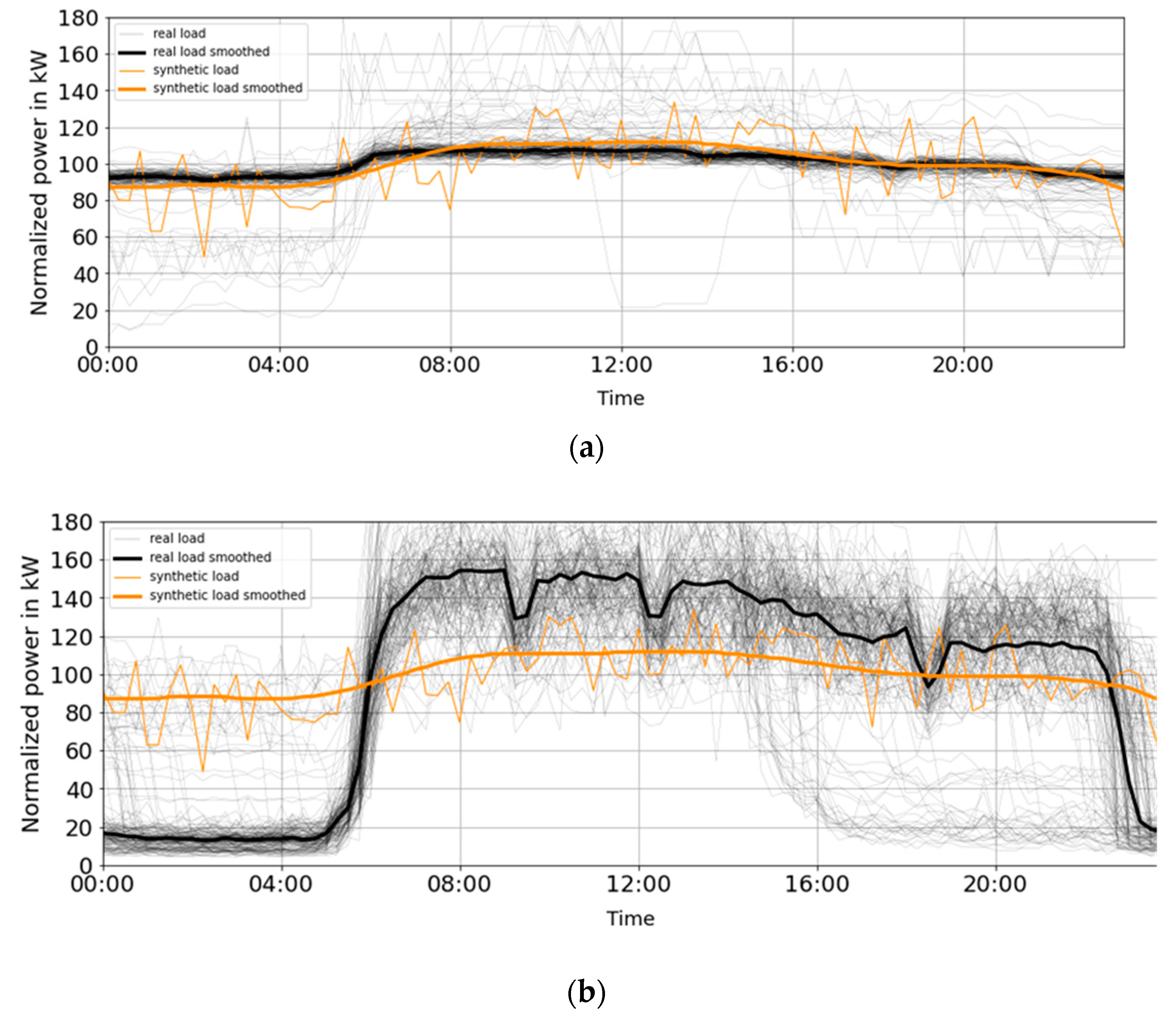
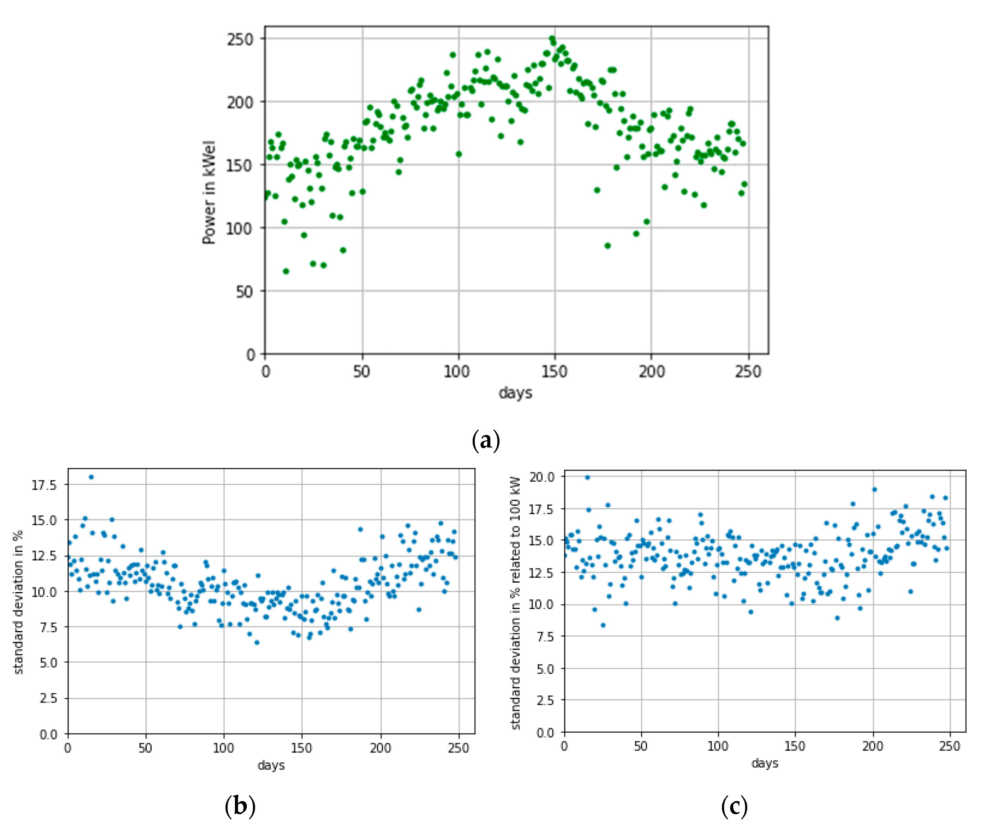
3.5. Step 4: Applying a Fluctuation Rate

Electrical load demand is hardly ever constant. With an increasing number of devices that are switched on and off constantly, the load profile fluctuates to varying degrees. In industrial plants, discontinuous operated mechanical devices especially cause these fluctuations due to their definition in Table 3. In this work, standard deviations of fluctuating real load data (confidential and therefore only described in general terms) were first calculated and then applied as synthetic fluctuations on the partial load of a discontinuous mechanical drive.

In total, 31 real load datasets are available, but only 11 of them correspond to the industry types investigated in this paper (

Table 5. List of available datasets of real industrial load profiles, their associated industry types and the numbers of shifts applied in the company.

Dataset No.	Industry Type	Number of Shifts
1	10.13 (meat processing)	3
2	25.61 (surface finishing and heat treating)	3
3	25.61 (surface finishing and heat treating)	1–3
4	25.62 (mechanics)	3
5	25.62 (mechanics)	2
6	25.62 (mechanics)	3
7	25.62 (mechanics)	1–2
8	28 (machinery)	2
9	28 (machinery)	2
10	28 (machinery)	2
11	28 (machinery)	3
12–31	Other industry types

). Each dataset consists of a time series of the total electricity demand of the company (active power at the transfer meter) in kW over a period of one to three years with a resolution of 15 min. In Figure 8, weekly real load profiles are plotted from four exemplary industries.

To calculate the standard deviation of each dataset, first the non-working days (Saturdays, Sundays, holidays and “bridging days”) were excluded from the total time series because load profiles of non-working days differ from working days, as can be observed in Figure 8.

Additionally, production periods differ with the different shift patterns of companies. Therefore, the standard deviation was calculated for the load only during production times. The daily time window for analysis was narrowed down to one hour after the start of the shift until one hour before the end of the shift, as summarized in

Table 6. Time periods for determining the standard deviation of the power demand.

	1 Shift 8:00 to 16:00	2 Shift 6:00 to 22:00	3 Shift 00:00 to 24:00
Monday–Thursday	9:00 to 15:00	7:00 to 21:00	00:00 to 24:00
Friday	9:00 to 15:00	7:00 to 14:00	00:00 to 21:00
Saturday, Sunday, holidays, bridging days	No analysis	No analysis	No analysis

. Of all industries analyzed, eight ran their production in one shift, nine ran their production in two shifts, 13 ran their production in three shifts and one alternated between one- and two-shift patterns.

By default, the standard deviation is related to the mean value of all considered values. However, since the trend of the load profiles was not constant, this approach would have resulted in a standard deviation not only reflecting the fluctuation but also being influenced by the trend itself. To avoid this, the standard deviation was related to the trend, which was generated by smoothing the original load curve by using LOWESS (the weighted linear least squares regression) over the span of 0.5.

Figure 9 shows an example of the 24 h electricity consumption of a 2-shift mechanic company and the smoothed profile for the examined time range between 7:00 and 21:00.

The relative standard deviation was calculated for each working day j with

$$s_j=\frac{\sqrt{\frac{1}{N-1}{{\displaystyle \sum }}_{i=1}^N{\left(x_i-x_{i,\mathrm{smoothed}}\right)}^2}}{{\overline{x}}_j}\times 100\%$$

(13)

where s_j is the relative standard deviation of one working day j in %, N is the number of values of time windows, i is one time point, x_i and x_i,smoothed are the original and smoothed power demands of the real dataset in kW, respectively, and ${\overline{x}}_j$ is the average power of the time windows. As the standard deviations are not directly proportional to the power consumption, the s_j was converted into

$$s_{ref, j}=s_j\times \sqrt{\frac{{\overline{x}}_j}{100 \mathrm{kW}}}$$

(14)

by relating the standard deviation to a fixed average consumption of 100 kW.

Equation (14) is based on the central limit theorem of Lindberg–Lévy [71]. Finally, the median s_ref of all s_ref,j was calculated. For the industry types with more than one dataset, the average of all s_ref was calculated, which represented the fluctuation height of the associated industry type. For the industry types without any real load datasets, the average fluctuation height of all 31 available datasets was calculated and applied.

Table 7. Fluctuation heights of industry types.

WZ 2008 Code	Name of Industry Type	Fluctuation Height
		sref in %
10.13	Meat processing	14
25.61	Surface finishing and heat treating	19
25.62	Mechanics	13
28	Machinery	11
All other industry types		19

shows the fluctuations for four industry types and the average fluctuation for the remaining industry types.

To apply the standard deviation to the synthetic profiles, first, a series of 96 random numbers of a Gaussian normal distribution was generated (one value for every 15 min of one day; mean value = 0 and standard deviation = s_ref). Although the standard deviation was calculated from the total active power consumption of the plant, for a graphical representation of the synthetic load profiles, the fluctuation was applied to only the profile of the discontinuous mechanical drive (Figure 10). Therefore, the series of random numbers r_i with the unit kW was added to the time series of the discontinuous mechanical drive y_{MD_disconti}, resulting in a new time series for discontinuous mechanical drive:

$$y_{MD\_disconti+fluc, i}=y_{\mathrm{MD}\_\mathrm{disconti},i}+r_i$$

(15)

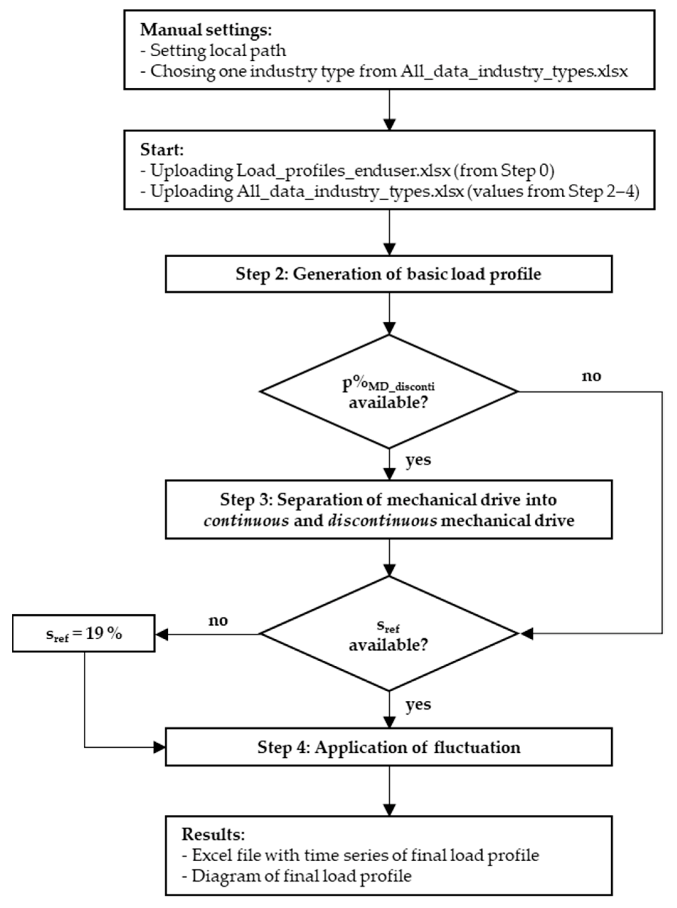
3.6. Model Development

The tool was written in Python and was released in the GitHub repository: https://github.com/asandhaa/SyntheticLoadProfiles (accessed on 1 May 2022).

Figure 11 shows the structure of the model. The Python scripts for the generation of synthetical load profiles can be applied to any industry type. The input data was collected in two Excel files. The first file contains the time series for the normalized end-user profiles and the second file contains all the data collected for the 11 industry types defined so far. For the addition of further industry types (defined by using Step 1), only the corresponding data (Steps 2–4) for this industry type were added to the second Excel file, and with the help of the code Python, a synthetic load profile was created. We would appreciate if other scientists would contribute to the data collection in order to cover the industry sector completely.

4. Benefits and Limits of the Presented Methodology

The time span of the load profiles was intentionally restricted to one typical working day as the focus was on generating the profiles with precise data contents and a characteristic course. For the generation of longer time spans, normalized end-user profiles (Step 0) would have had to first be generated for further types of days, such as weekends and closing days, and seasonal effects would have also had to be included for entire years.

4.1. Step 0: Normalized Load Profiles for Eight End-Use Appliances

Unlike most published synthetic load profiles for which only the absolute demand is modeled, the synthetic load profiles in this study were further separated into loads for different end users in industries. The AGEB [57] publishes the energy balances of the whole German industry classified into 14 categories on a yearly basis by using similar end-use categories. The shares of the end users are shown in Figure 12. The energy demands of the different end users will gain importance in the future as the integration of more and more renewable energies into the German energy system with a simultaneous reduction of fossil fuels will cause an increasing electrification of industrial applications [2,9,72,73]. As a result, the shares of the end users will change significantly as the electrification of the heat supply will increase more strongly than that of other applications [9]. Dividing the total electricity demand into end users is a major advantage of this method because the individual end users can be adapted independently to different scenarios of future energy supply. Therefore, the presented load profiles are optimal to represent the industry demands for energy system analyses with regard to electrification, flexibility (DSM) and storage technology studies. In the year 2019, the dominating electrical end users in the German industry were mechanical drive (72%) followed by process heat (13%) [57]. The end-user categories space heating and hot water consumed, respectively, less than 1% of the electricity in most industries and can theoretically be neglected in this method. Alternatively, hot water can be merged with process heat and space heating, and space cooling can be combined into an aggregated end user, such as HVAC, as a lot of literature sources publish space climatization as HVAC anyway. The advantage of using an HVAC end user is that in a future step, the user’s normalized load profile could be related to the outside temperature profile for one day and/or over one year.

As far as the course of the profiles is concerned, it was assumed that this depended on the application and not on the industry type. This generalization may certainly not apply to every industry type, but on the one hand, it ensures that the final profiles of the industries differ slightly in their courses, and on the other hand, it gives us the possibility of adjusting the end-user profiles individually at any time based on new findings.

4.2. Step 1: Clustering into Industry Types

The biggest advantage of clustering the industry types according to the WZ 2008 system is that the energy data, application balances and locations of companies refer to this classification. In addition, the sub-sectors are transferable to other classification systems if data from outside Germany are used. International energy data are often published with regard to the International Standard Industrial Classification of all economic activities (ISIC) Rev. 4 [40], and the corresponding ISIC code is given for each sub-sector in the WZ 2008 classification.

4.2.1. Industry Types out of the Division 10 Food Products

In the food industry, a wide variety of different production processes is encountered, corresponding to the range of different products that are produced. Companies at the 3- and 4-digit levels are homogeneous to a high degree because food companies often produce only one or a few specific food products. This, together with a good availability of energy balances for individual plants, is in favor of defining industry types at the 3- and 4-digit levels. Therefore, numerous studies of individual food sector plants [53,60,61,63,64,74] are scaled up to their corresponding industry types.

To determine the benefits of classifying the industry types of the 3- and 4-digit levels, the four generated profiles were to be compared to the synthetic load profile of the parental 2-digit-levels 10, 11 and 12 (food, beverages and tobacco) [57]. The synthetic profile was generated by using Steps 1, 2 and 4. Step 3 requires homogenous processes in companies, which was not given in this level. Comparing the load profiles of Figure 13, it can be seen that the distribution of the end users differs a lot between the four selected industry types as well as compared to the profile of the division level. For example, process cooling is needed in all of the regarded industry types, but slaughterhouses need more than half of their electricity consumptions for this purpose. However, process heat plays a much bigger role for bakeries than for the other branches. The amount of the discontinuous processes varies between 5.6% for 10.7 (baked goods) and 20.2% for 10.13 (meat processing). These differences in the load profiles clearly prove the need for a widely branched food industry.

4.2.2. Industry Types out of the Division 25 Metal Products

If the biggest end-user mechanical drive was excluded, the six synthetic load profiles of the metal product division were similar (Figure 14) as the share of electricity for the end users was obtained from the same source (Table 2). However, the different shares of discontinuous mechanical drives (30% for 25.61 (surface finishing) up to 90% for 25.5 (production of forgings, etc.)) and the applied fluctuations ensured individual load profiles for the different industry types. For this reason, it was advantageous in this case to split the department into further industry types even though the data situation for the end users was poor.

4.2.3. Industry Type 28 (Machinery)

For the mechanical engineering sector, the research revealed that on the one hand, the heterogeneous industrial landscape calls for a very finely separated industrial sector, but on the other hand, this sector lacks the data basis for actually implementing this separation. Therefore, the machinery sector was not disaggregated further and the entire division was represented by one aggregated profile (Figure 15). However, the advantage of generating a synthetic load profile for a division was a good data availability for the end-user shares in the second step [57] and a regional energy demand at the NUTS-3 level [75].

4.3. Step 2: Generating a Basic Load Profile

After the second step, a base load profile had already been generated, the surface of which had been roughened in the final step by imposing fluctuations with the help of real data, but the overall characteristic curve remained the same. These base profiles were therefore well suited for quantitative comparisons with the courses of smoothed real profiles. To check the accuracies of the resulting synthetic load profiles, the root mean square error (RMSEs) between synthetic and real loads (cf. the datasets listed in Table 5) were calculated. In the case of the synthetic profiles, the absolute daily load $y_i$ after Step 2 was taken before the fluctuation was applied. In the case of the real load profiles, the datasets were smoothed as follows: First, only the total power consumption of the working days Tuesday, Wednesday and Thursday (excluding holidays) was isolated from the entire time series. Since these days were embedded between other working days, their base loads were not affected by preceding or succeeding production breaks and their load patterns were quite similar, as can be observed in Figure 8. The time series $x_{j }$for each day j were normalized to an average consumption of 100 kW by using

$$x_{ij, norm }=\frac{x_{ij}}{\overline{x_j}}\times 100 \mathrm{kW}$$

(16)

where i (i = 1,…,n; n = 96 values) is a time point in 24 h, and then the series were plotted on top of each other (Figure 16). To smooth the fluctuating curve, the method from Section 3.5 (LOWESS) could not be applied for the whole day as the abrupt increase and decrease of power consumption at the beginning and end of a shift would not be correctly displayed by using this method. Therefore, the median of all values at time point i was calculated. The resulting time series $x_{i, smoothed}$ represented the profile of the smoothed curve.

The RMSE between the synthetic load profile y_i and the smoothed real load profile x_i,norm was calculated by using

$$\mathrm{RMSE}=\sqrt{\frac{{{\displaystyle \sum }}_{i=1}^n{\left(x_{i,smoothed}-y_i\right)}^2}{n}}$$

(17)

The resulting RMSE values are shown in

Table 8. RMSE between real and synthetic industrial profiles and the number of shifts of the investigated companies.

Dataset No.	Industry Type	Number of Shifts	RMSE in kW
1	10.13 (meat processing)	3	7.19
2	25.61 (surface finishing and heat treating)	3	4.73
3	25.61 (surface finishing and heat treating)	1	14.13
4	25.62 (mechanics)	3	2.75
5	25.62 (mechanics)	2	5.84
6	25.62 (mechanics)	3	6.48
7	25.62 (mechanics)	1.2	42.62
8	28 (machinery)	2	11.34
9	28 (machinery)	3	19.55
10	28 (machinery)	3	6.63
11	28 (machinery)	1	5.84

and graphed in Figure 16.

The values of the calculated RMSE were distributed quite independently of the industrial types between 3 kW and 43 kW of the absolute value. Above all, one correlation was obvious: the quality of the synthetic profiles was particularly good and had a low RMSE when a plant operated in 3 shifts for datasets 1, 2, 4, 6 and 11. This correlation can be seen especially in the comparison of the course of the real profile of dataset 4 with the synthetic profile of the corresponding industry type 25.62 in Figure 16a, which had the lowest RMSE of 2.75. The load profiles of dataset 7 show a particularly high RMSE (Figure 16b). Outside the shift times, the base load dropped to about 10% of the production load. For a more accurate representation of the profiles, the applied shiftwork times of the industry types had to be integrated into the methodology. For this, the resulting load profiles had to be stretched vertically at the times of the shift starts and shift ends. The factor between the peak load during the work shift and the baseload outside the production time could be determined from the real data and applied across the board for all industry types or calculated individually from the respective datasets for the different industry types. However, it is important to note that the companies of an industry type did not all use the same shift times (see Table 8), and in order to model the regional electricity demand of an industry type, it was therefore essential to also specify the distribution of one-, two- and three-shift companies of the particular industry type.

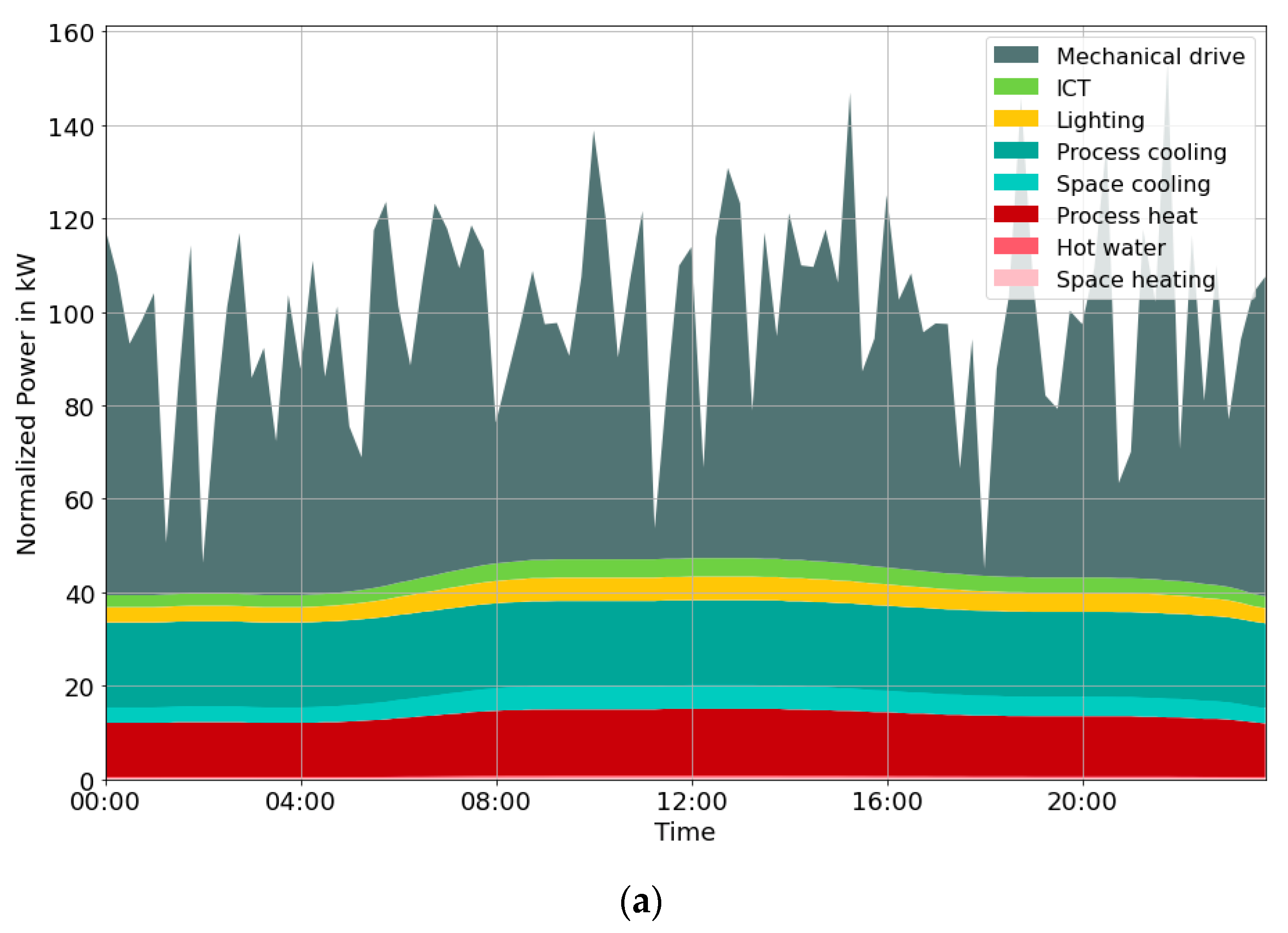
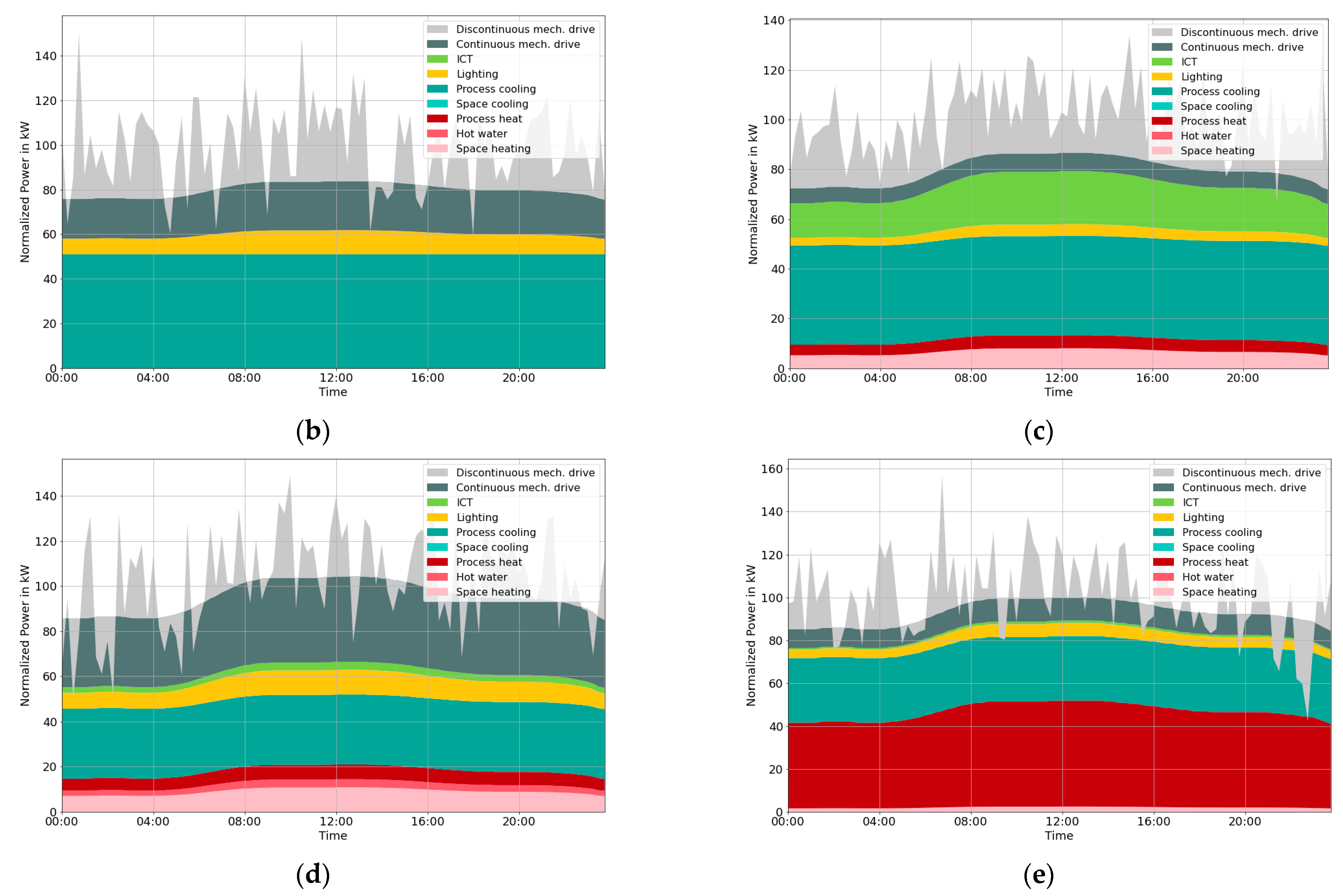
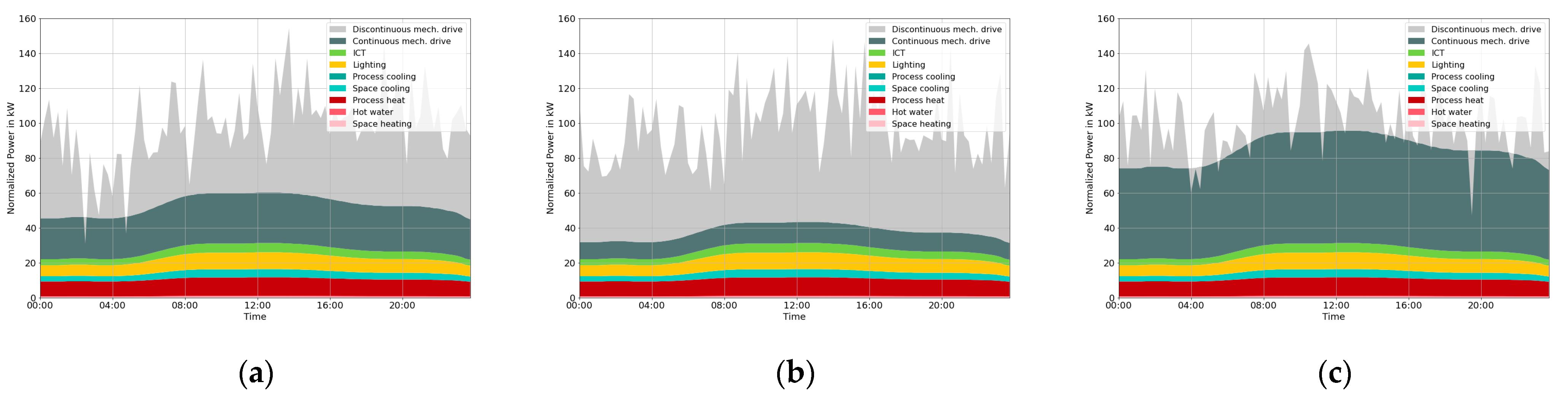
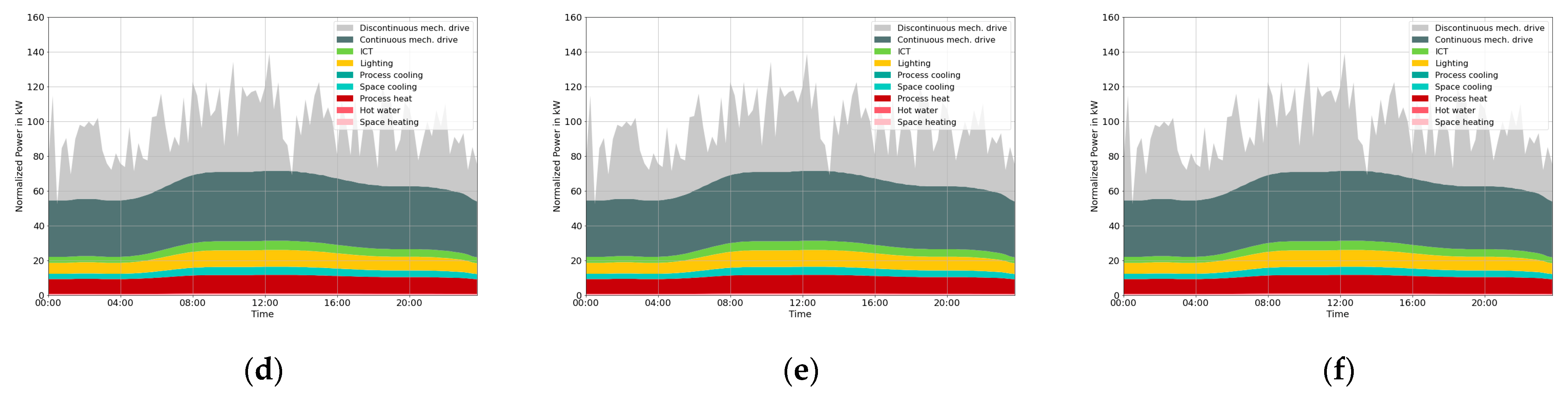
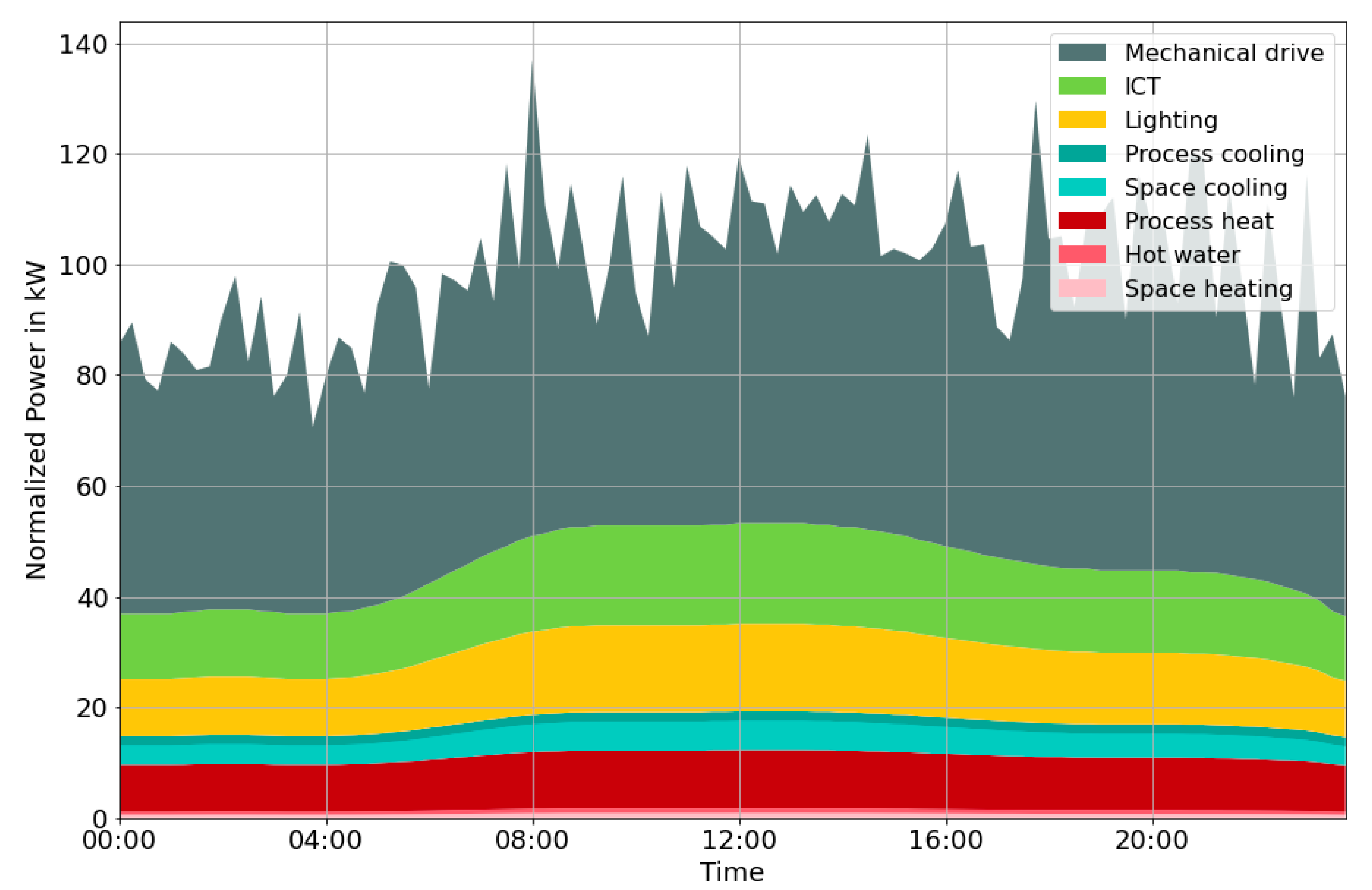
4.4. Step 3: Classifying Mechanical Drive Processes

The classification of mechanical drive processes into continuous and discontinuous process types was, unlike the previous steps, done by using a bottom-up approach by analyzing representative companies and applying the result to a whole industry type. The energy demands of the typical processes of the food industries could all be covered by the literature. Although numerous processes of the metal product industries are listed in large numbers in the literature and on specific websites [68,69,70,76,77], their proportions of energy consumption have hardly been published at all. For all but one industry type, our own assumptions about the processes’ energy demands had to be made in this approach. For industry type 25.62 (mechanics), access to the electricity meters of all the machines of one company was available, and the classification and quantitative power demands could be determined with high accuracies. For industry type 28 (machinery), which unified more than 6000 companies [51], one company could not represent the whole division. Therefore, Step 3 was skipped for this industry type.

For analyzing flexibility potentials for future energy systems, the continuous and discontinuous mechanical drive profiles could be handled differently based on their demand-side management products (Table 3). This allows the use of different flexibility products to be directly linked to the corresponding shares of the total loads; e.g., a sudden switching on and off can be realized only by using the load of a discontinuous mechanical drive. This categorization is the first step for separating loads for the purpose of a flexibility evaluation. In the future, Step 3 can be applied to the second-largest electricity consumer process heat as well. Up to now, its main energy source has been natural gas at almost 50% [57], but due to the predicted electrification of process-heat applications [9], e.g., for certain low-temperature energy needs, such as curing and drying [77], its electricity demand is about to increase. The classification of process-heat applications can be performed, e.g., on technologies or temperature levels.

4.5. Step 4: Applying a Fluctuation Rate

Applying a synthetic fluctuation made the profiles more realistic. The fluctuations increased the complexity of the demand and challenged the model to adapt the power supply to the fluctuations or to use batteries for balancing. Additionally, the applied fluctuation served as a stochastic attribute in the method. Every time a load profile was generated, the random numbers ensured a unique synthetic load profile per industry type.

The resulting profiles in Figure 13 and Figure 14 show that although the calculated share of discontinuous mechanical drives and the range of fluctuation were obtained from different sources, in all cases in which real data were available, the fluctuation range was smaller than the partial load. For some of the profiles, e.g. 10.5 (dairy products; Figure 13d) and 10.7 (baked goods; Figure 13e), the imposed fluctuation did not only remain within the load of the discontinuous mechanical drive but also immersed into the underlying end users. This was because the average fluctuation range of 19% was higher than the electricity demands of the discontinuous mechanical processes (Table 4). This observation did not occur for the four profiles out of the metal production industry to which the 19% fluctuation was applied (Figure 14). This was because the proportions of the discontinuous mechanical processes were bigger (min. 46% of the total electricity demand) than the applied fluctuation. Step 4 should be modified in a future work so that for those profiles without any real datasets, the fluctuation height is not calculated from the average of all fluctuations but is proportional to the amount of the discontinuous mechanical drives.

An important property of white noise must be considered, especially when scaling the load profiles to a given power level: the fluctuation range is not proportional to the power level. That is why the calculated standard deviation of the real load profiles was further modified by using Equation (14) in order to adjust the fluctuation to a reference mean power demand of 100 kW. In this study, a reference value of 100 kW was used because in that case, the absolute and relative fluctuation have the same values, and conversions of one unit to the other are simplified. With an increasing absolute power consumption, the relative fluctuation becomes smaller according to the central limit theorem [71] by Lindberg–Lévy. For example, if a company’s power consumption of one day is twice that of the previous day, the relative standard deviation is lower by the root of two. This effect is shown in Figure 17. In Figure 17a, the average daily power consumption of a meat processing company of one year is plotted against the number of days. It clearly shows the increased power demand during the summer. The relative fluctuation in Figure 17b exhibits a contrary course, with low values during the summer months. However, if the daily standard deviations were normalized to a daily average consumption of 100 kW by using Equation (14), the values would not be influenced by the power, as can be seen in Figure 17c. Without this step, the standard deviations of different days or different companies could not be compared with each other.

5. Regional Representation of Industrial Electricity Demand

The goal of our research was to evaluate a method for generating detailed spatial, temporal and sectoral industrial load profiles for energy system modeling. Up to now, the presented methodology has covered only the temporal and sectoral aspects. However, since in this method, the application of synthetic fluctuations is used, in this chapter, some words should be said about the correct dimensioning of this quantity for the regionally adjusted load profiles. To integrate the generated load profiles in energy-system models for the representation of spatial industrial electricity demands, the normalized profiles have to be dimensioned for the specific region. First, the regional electricity demand of one industry type has to be researched from the company registers of the federal statistical office [78] or state offices and the average weekday power demand $\overline{x}$ has to be evaluated in kW. As the partial loads were adjusted to a total average electricity consumption of 100 kW, the quotient of the resulting value and 100 kW had to be multiplied with each time series of the end-user loads. As for the fluctuation range, it has to be adapted to the real consumption by using the inverse equation of Equation (14):

$$s=s_{ref}\times \sqrt{\frac{100\mathrm{kW}}{\overline{x}}}$$

(18)

and applied to the discontinuous mechanical drive load, where s is the regional fluctuation range for industrial load and s_ref is the calculated fluctuation range relative to 100 kW (Table 7). After the dimensioning of the individual load profiles, the whole industrial electricity demand of the region in question can be reflected by using a simple summation of all the industry types occurring in this region. Since the fluctuations were generated using random numbers, the addition caused the relative fluctuation of the regional profile to decrease, like it does in reality.

Unfortunately, the availability of energy data for industrial types at the four-digit level were publicly available for only Germany as a whole. For the two-digit sectors, however, data were available down to the NUTS-3 level, and the regional distribution could be realized by using the method of DemandRegio [13]. However, to map highly decomposed industries, such as the food industry, to small regions, assumptions had to be made top-down or by researching the local companies and classifying them in four-digit sectors. The highly resolved spatial mapping of the demand with the integration of the correct scaling of the fluctuation ranges is a task for upcoming work.

6. Conclusions and Future Work

In this paper, a methodology was described for generating industrial electrical load profiles for different industry sectors in a high temporal and sectoral resolution. The method was structured in four consecutive steps. In addition to a characteristic daily load shape, the final synthetical load profiles included information about the electricity demands of end-use appliances and mechanical drive processes.

Industry types were selected from different levels of the classification system WZ 2008 [41]. The goal was to generate synthetic load profiles for as homogeneous industry types as possible. It was proven that this clustering process is necessary for the food industry as the defined industry types differ greatly from each other and from the aggregated food industry with regard to end products and electricity applications. However, it also became clear that this approach reaches its limits when a highly heterogeneous industry, such as mechanical engineering, cannot be disaggregated down further due to scarce data.

Eight electrical end-user categories (space heating, hot water, process heat, space cooling, process cooling, lighting, information and communications technologies and mechanical drives) were defined to which one of three modeled daily normalized load profiles was assigned. The basic daily profile of one industry type was created by stacking the eight end-user profiles with their industry-type-specific proportions. A quantitative comparison of the basic load profiles with real load profiles was done by calculating the RMSE of the two profiles. It was found that the RMSE is particularly low when the real profiles are obtained from 3-shift operating companies. This means that the method is very well suited for the representation of loads from 3-shift operations, but the profiles have to be adapted for 1- or 2-shift operations. For this purpose, the base load profiles are to be modified on the basis of the typical number of working shifts of the respective industry type.

Furthermore, the mechanical drive processes were classified into continuous and discontinuous categories, and the load was separated according to the shares of these two categories. These two categories deliver different DSM potentials, and flexibility evaluation can be performed in energy-system models. The classification of the processes requires ample data, which is abundantly given for the food sector; is mostly available in a qualitative form for metal products, although the electricity requirements of the processes have to be estimated for the most part, and proves to be rather complex for the mechanical engineering sector.

In the last step, a fluctuation range was calculated from a real load data and applied to the synthetic load profile as white noise. This application made the profiles more realistic, and short-time flexibility modeling could be realized in an energy system analysis. Additionally, the applied fluctuation served as a stochastic attribute in the method. Every time a load profile is generated, the random numbers ensure a unique synthetic load profile per industry type.

This methodology is particularly well suited for reflecting the demands of different industry types in power system modeling and adjusting them according to specified future scenarios. Due to the high temporal resolution, the use of renewable energies can be optimized more precisely. The sectoral clustering of the industry sector allows a precise locational positioning of the industry; it can therefore reflect the regional demand more accurately and can thus optimize the expansion of renewable energy regionally in system modeling. By separating the total load into different end users, and especially the mechanical drive, into continuous and discontinuous processes, it is possible for flexibility products, such as load regulation, to be applied to only those end-user loads that are eligible for it. For example, a sudden switching on and off can be applied only to the discontinuous mechanical-drive load. The applied fluctuation adds a stochastic component to the demand and increases the complexity of the model.

The method was applied to the divisions of WZ 2008 C:10 food products, 25 metal products and 28 machineries, which were broken down into a total of 11 industry types. These generated load profiles are already used in the energy system mode MyPyPSA-Ger [30]. The code for creating the profiles with its input data can be accessed openly in GitHub. The synthetic load profiles for industry types from the remaining 21 divisions will be gradually implemented. We are grateful for any contributions from the scientific community to help us finalize the compilation of the data.

References

1. Schlesinger, M.; Lindenberger, D.; Lutz, C. Entwicklung der Energiemärkte—Energiereferenzprognose: Studie im Auftrag des Bundesministeriums für Wirtschaft und Technologie; Federal Ministry for Economic Affairs and Climate Action: Berlin, Germany, 2014.
2. Sterchele, P.; Brandes, J.; Heilig, J.; Wrede, D.; Kost, C.; Schlegl, T.; Bett, A.; Henning, H.-M. Wege Zu Einem klimaneutralen Energiesystem: Die Deutsche Energiewende im Kontext Gesellschaftlicher Verhaltensweisen; Fraunhofer Institute for Solar Energy Systems: Freiburg, Germany, 2020. [Google Scholar]
3. Henning, H.-M.; Palzer, A. Was Kostet Die Energiewende? Fraunhofer Institute for Solar Energy Systems: Freiburg, Germany, 2015. [Google Scholar]
4. Stiftung Klimaneutralität; Agora Energiewende; Agora Verkehrswende. Klimaneutrales Deutschland 2045: Wie Deutschland seine Klimaziele Schon vor 2050 Erreichen Kann. Available online: https://www.agora-energiewende.de/veroeffentlichungen/klimaneutrales-deutschland-2045/ (accessed on 16 November 2021).
5. Sauer, A.; Abele, E.; Buhl, H.U. Energieflexibilität in der Deutschen Industrie: Ergebnisse aus dem Kopernikus-Projekt—Synchronisierte und Energieadaptive Produktionstechnik zur Flexiblen Ausrichtung von Industrieprozessen auf Eine fluktuierende Energieversorgung; SynErgie; Fraunhofer Verlag: Stuttgart, Germany, 2019; ISBN 978-3-8396-1479-2. [Google Scholar]
6. Benndorf, R.; Bernicke, M.; Bertram, A.; Butz, W.; Dettling, F.; Drotleff, J.; Elsner, C.; Fee, E.; Gabler, C.; Galander, C.; et al. Treibhausgasneutrales Deutschland im Jahr 2050, Dessau. 2013. Available online: https://www.umweltbundesamt.de/sites/default/files/medien/376/publikationen/treibhausgasneutrales_deutschland_im_jahr_2050_langfassung.pdf (accessed on 14 January 2021).
7. Öko-Institut; Fraunhofer ISI. Klimaschutzszenario 2050: Studie im Auftrag des Bundesministeriums für Umwelt, Naturschutz, Bau und Reaktorsicherheit; Öko-Institut: Berlin, Germany; Fraunhofer ISI: Berlin, Germany, 2015; Available online: https://www.oeko.de/oekodoc/2451/2015-608-de.pdf (accessed on 1 May 2022).
8. Elsland, R.; Boßmann, T.; Klingler, A.-L.; Herbst, A.; Klobasa, M.; Wietschel, M. Netzentwicklungsplan Strom: Entwicklung der regionalen Stromnachfrage und Lastprofile. 2016. Available online: https://www.isi.fraunhofer.de/content/dam/isi/dokumente/cce/2017/Fraunhofer_ISI_2017_Netzentwicklungsplan_Strom.pdf (accessed on 10 May 2022).
9. Ausfelder, F.; Drake, F.-D.; Erlach, B.; Fischedick, M.; Henning, H.-M.; Kost, C.; Münch, W.; Pittel, K.; Rehtanz, C.; Sauer, J.; et al. “Sektorkopplung”—Untersuchungen und Überlegungen zur Entwicklung eines integrierten Energiesystems; acatech: Munich, Germany, 2017; ISBN 978-3-9817048-9-1. [Google Scholar]
10. Umweltbundesamt. Energieverbrauch nach Energieträgern und Sektoren. Available online: https://www.umweltbundesamt.de/daten/energie/energieverbrauch-nach-energietraegern-sektoren#allgemeine-entwicklung-und-einflussfaktoren (accessed on 3 November 2021).
11. Bundesverband der Energie; Wasserwirtschaft e.V.; Verband kommunaler Unternehmen e.V.; Groupement Européen des entreprises et Organismes de Distribution d’Énergie. Abwicklung von Standardlastprofilen Gas. Available online: https://www.enwg-veroeffentlichungen.de/badtoelz/Netze/Gasnetz/Netzbeschreibung/LF-Abwicklung-von-Standardlastprofilen-Gas-20110630-final.pdf (accessed on 27 September 2021).
12. Guminski, A.; Hübner, T.; Rouyrre, E.; von Roon, S.; Schimmel, M.; Achtelik, C.; Rhiemeier, J.-M.; Fahl, U.; Bailey, I. Energiewende in der Industrie: Potenziale und Wechselwirkungen mit dem Energiesektor. Final Report. Available online: https://www.bmwk.de/Redaktion/DE/Downloads/E/energiewende-in-der-industrie.pdf?__blob=publicationFile&v=8 (accessed on 1 May 2022).
13. Gotzens, F.; Gillessen, B.; Burges, S.; Hennings, W.; Müller-Kirchenbauer, J.; Seim, S.; Verwiebe, P.; Tobias, S.; Jetter, F.; Limmer, T. DemandRegio: Harmonisierung und Entwicklung von Verfahren zur regionalen und zeitlichen Auflösung von Energienachfragen. Final Report. 2020. Available online: https://openaccess.ffe.de/wp-content/uploads/2020/12/DemandRegio_Abschlussbericht.pdf (accessed on 1 May 2022).
14. Seim, S.; Verwiebe, P.; Blech, K.; Gerwin, C.; Müller-Kirchenbauer, J. Die Datenlandschaft der deutschen Energiewirtschaft; Working Paper; Zenodo: Meyrin, Switzerland, 2019. [Google Scholar]
15. Ringkjøb, H.-K.; Haugan, P.M.; Solbrekke, I.M. A review of modelling tools for energy and electricity systems with large shares of variable renewables. Renew. Sustain. Energy Rev. 2018, 96, 440–459. [Google Scholar] [CrossRef]
16. Calliope: A Multi-Scale Energy Systems Modelling Framework. Available online: https://calliope.readthedocs.io/en/stable/user/introduction.html (accessed on 8 September 2020).
17. Lise, W.; Sijm, J.; Hobbs, B.F. The Impact of the EU ETS on Prices, Profits and Emissions in the Power Sector: Simulation Results with the COMPETES EU20 Model. Environ. Resour. Econ. 2010, 47, 23–44. [Google Scholar] [CrossRef]
18. Neon. EMMA Dokumentation. Available online: https://neon.energy/emma-documentation.pdf (accessed on 1 May 2022).
19. Stockholm Environment Institute. Introduction NEMO. Available online: https://sei-international.github.io/NemoMod.jl/stable/ (accessed on 22 November 2021).
20. Blair, N.; DiOrio, N.; Freeman, J.; Gilman, P.; Janzou, S.; Neises, T.; Wagner, M. System Advisor Model (SAM) General Description (Version 2017.9.5); National Renewable Energy Laboratory: Golden, CO, USA, 2018. Available online: https://www.nrel.gov/docs/fy18osti/70414.pdf (accessed on 22 November 2021).
21. Wiese, F. Renpass—Renewable Energy Pathways Simulation System. Available online: https://www.uni-flensburg.de/eum/forschung/abgeschlossene-projekte/renpass/ (accessed on 1 May 2022).
22. ENTSO-E Transparency Platform. Available online: https://transparency.entsoe.eu/ (accessed on 28 July 2021).
23. urbs: A Linear Optimisation Model for Distributed Energy Systems. Overview Model Structure. Available online: https://urbs.readthedocs.io/en/latest/users_guide/overview.html (accessed on 20 November 2021).
24. Lambert, T.; Gilman, P.; Lilienthal, P. Micropower System Modeling with HOMER. Integr. Altern. Sources Energy 2006, 1, 379–417. [Google Scholar]
25. Johnston, J.; Henriquez-Auba, R.; Maluenda, B.; Fripp, M. Switch 2.0: A modern platform for planning high-renewable power systems. SoftwareX 2019, 10, 100251. [Google Scholar] [CrossRef]
26. Center for Sustainable Energy Systems; Reiner Lemoine Institute. oemof/demandlib. 2014. Available online: https://oemof.readthedocs.io/en/latest/ (accessed on 8 November 2021).
27. Center for Sustainable Energy Systems; Reiner Lemoine Institute. oemof/demandlib. 2014. Available online: https://demandlib.readthedocs.io/en/latest/bdew.html#id1 (accessed on 22 October 2021).
28. Erlach, B.; Henning, H.M.; Kost, C.; Palzer, A.; Stephanos, C. Optimierungsmodell REMod-D. Materialien zur Analyse »Sektorkopplung«–Untersuchungen und Überlegungen zur Entwicklung eines integrierten Energiesystems; Schriftenreihe Energiesysteme der Zukunft: München, Germany, 2018. [Google Scholar]
29. E3 Modelling. PRIMES.; National Technical University: Athens, Greece; Available online: https://e3modelling.com/modelling-tools/primes/ (accessed on 21 October 2021).
30. Abuzayed, A.; Hartmann, N. MyPyPSA-Ger: Introducing CO2 taxes on a multi-regional myopic roadmap of the German electricity system towards achieving the 1.5 °C target by 2050. Appl. Energy 2022, 310, 118576. [Google Scholar] [CrossRef]
31. Hörsch, J.; Hofmann, F.; Schlachtberger, D.; Brown, T. PyPSA-Eur: An open optimisation model of the European transmission system. Energy Strategy Rev. 2018, 22, 207–215. [Google Scholar] [CrossRef] [Green Version]
32. GCAM (The Global Change Analysis Model) Documentation: Demand for Energy. Available online: http://jgcri.github.io/gcam-doc/demand_energy.html (accessed on 19 November 2021).
33. Luderer, G.; Leimbach, M.; Bauer, N.; Kriegler, E.; Baumstark, L.; Bertram, C.; Giannousakis, A.; Hilaire, J.; Klein, D.; Levesque, A.; et al. Description of the REMIND model (version 1.6). Available online: https://www.pik-potsdam.de/en/institute/departments/transformation-pathways/models/remind/remind16_description_2015_11_30_final (accessed on 19 November 2021).
34. LIBEMOD—Frischsenteret. Available online: https://www.frisch.uio.no/ressurser/LIBEMOD/ (accessed on 20 November 2021).
35. Open Energy Information. RETScreen Clean Energy Project Analysis Software. Available online: https://openei.org/wiki/RETScreen_Clean_Energy_Project_Analysis_Software (accessed on 22 November 2021).
36. Burandt, T.; Löffler, K.; Hainsch, K. GENeSYS-MOD v2.0—Enhancing the Global Energy System Model: Model Improvements, Framework Changes, and European Data Set; Deutsches Institut für Wirtschaftsforschung (DIW): Berlin, Germany, 2018. [Google Scholar]
37. Haasz, T. Entwicklung von Methoden zur Abbildung von Demand Side Management in Einem Optimierenden Energiesystemmodell: Fallbeispiele für Deutschland in den Sektoren Industrie, Gewerbe, Handel, Dienstleistungen und Haushalte; Universität Stuttgart: Stuttgart, Germany, 2017; ISBN 0938-1228. [Google Scholar]
38. Kuder, R. Energieeffizienz in der Industrie: Modellgestützte Analyse des effizienten Energieeinsatzes in der EU-27 mit Fokus auf den Industriesektor. TIMES PanEU. 2014. Available online: https://elib.uni-stuttgart.de/bitstream/11682/2305/1/FB_115_Energieeffizienz_Ralf_Kuder.pdf (accessed on 1 May 2022).
39. The North American Industry Classification System. Available online: https://www.census.gov/naics/reference_files_tools/2017_NAICS_Manual.pdf (accessed on 1 May 2022).
40. UN. International Standard Industrial Classification of All Economic Activities (ISIC); Rev.4; United Nations: New York, NY, USA, 2008; ISBN 9211615186. [Google Scholar]
41. Statistisches Bundesamt. Klassifikation der Wirtschaftszweige: Mit Erläuterungen; Federal Office of Statistics: Wiesbaden, Germany, 2008. [Google Scholar]
42. Blesl, M.; Kessler, A. Energieeffizienz in der Industrie; Springer: Berlin/Heidelberg, Germany, 2017; ISBN 978-3-662-55998-7. [Google Scholar]
43. Starke, M.; Alkadi, N. Assessment of Industrial Load for Demand Response across U.S. Regions of the Western Interconnect; Oak Ridge National Laboratory: Oak Ridge, TN, USA, 2013. [Google Scholar]
44. Bernstein, R.; Madlener, R. Short- and long-run electricity demand elasticities at the subsectoral level: A cointegration analysis for German manufacturing industries. Energy Econ. 2015, 48, 178–187. [Google Scholar] [CrossRef]
45. Schmid, T. Dynamische und kleinräumige Modellierung der aktuellen und zukünftigen Energienachfrage und Stromerzeugung aus Erneuerbaren Energien. Ph.D. Thesis, Technische Universität München, München, Germany, 2019. [Google Scholar]
46. Hale, E.; Horsey, H.; Johnson, B.; Muratori, M.; Wilson, E.; Borlaug, B.; Christensen, C.; Farthing, A.; Hettinger, D.; Parker, A.; et al. The Demand-Side Grid (dsgrid) Model Documentation; NREL/TP-6A20-71492; National Renewable Energy Laboratory: Golden, CO, USA, 2018. [Google Scholar]
47. Alkadi, N.E.; Starke, M.R.; Ookie, M.; Nimbalkar, S.U.; Cox, D.F. Industrial Geospatial Analysis Tool for Energy Evaluation-IGATE-E; Oak Ridge National Laboratory: Oak Ridge, TN, USA, 2013. [Google Scholar]
48. Bureau, U.C. About Manufacturing Energy Consumption Survey (MECS). Available online: https://www.census.gov/programs-surveys/mecs/about.html (accessed on 23 November 2021).
49. Load Shape Library (LSL) 8.0; Electric Power Research Institute (EPRI): Washington, DC, USA, 2019.
50. Rohatgi, A. WebPlotDigitizer: Web Based Tool to Extract Data from Plots, Images, and Maps. Available online: https://automeris.io/WebPlotDigitizer (accessed on 24 September 2021).
51. Statistisches Bundesamt. Produzierendes Gewerbe: Beschäftigte, Umsatz und Investitionen der Unternehmen und Betriebe des Verarbeitenden Gewerbes sowie des Bergbaus und der Gewinnung von Steinen und Erden; Statistisches Bundesamt (Destatis): Weisbaden, Germany, 2018.
52. Statistisches Bundesamt. Beschäftigte, Umsatz und Investitionen des Verarbeitenden Gewerbes sowie des Bergbaus und der Gewinnung von Steinen und Erden—Fachserie 4 Reihe 4.2.1—2019; Federal Office of Statistics: Wiesbaden, Germany, 2019. [Google Scholar]
53. Brush, A.; Masanet, E.; Worrell, E. Energy Efficiency Improvement and Cost Saving Opportunities for the Dairy Processing Industry: An ENERGY STAR® Guide for Energy and Plant Managers; Lawrence Berkeley National Laboratory: Berkeley, CA, USA, 2011. [Google Scholar]
54. Gühl, S.; Schwarz, M.; Schimmel, M. Branchensteckbrief der Nahrungsmittelindustrie; Institut für Energiewirtschaft und Rationelle Energieanwendung: Stuttgart, Germany, 2019. [Google Scholar]
55. Nunes, J.; Da Silva, P.D.; Andrade, L.P.; Domingues, L.; Gaspar, P.D. Energy assessment of the Portuguese meat industry. Energy Effic. 2016, 9, 1163–1178. [Google Scholar] [CrossRef]
56. Statistisches Bundesamt. Energieverbrauch der Betriebe im Verarbeitenden Gewerbe: Deutschland, Jahre, Nutzung des Energieverbrauchs, Wirtschaftszweige, Energieträger: Tabelle: 43531-0002. Available online: https://www-genesis.destatis.de/genesis//online?operation=table&code=43531-0002&bypass=true&levelindex=0&levelid=1652428745306#abreadcrumb (accessed on 11 November 2021).
57. Fraunhofer ISI. Erstellung von Anwendungsbilanzen für die Jahre 2018 bis 2020 für die Sektoren Industrie und GHD; Fraunhofer ISI: Freiberg, Germany, 2019. [Google Scholar]
58. Energieinstitut der Wirtschaft GmbH. Effiziente Metallverarbeitung. Available online: https://www.energieinstitut.net/sites/default/files/metaller_dt_1905s.pdf (accessed on 1 May 2022).
59. VDMA. Mehr Energieeffizienz im Deutschen Maschinenbau: 26 Praxisbeispiele; Forum Energie: Frankfurt, Germany, 2014. [Google Scholar]
60. Feliciano, M.; Rodrigues, F.; Gonçalves, A.; Santos, J.; Leite, V. Assessment of Energy Use and Energy Efficiency in Two Portuguese Slaughterhouses. Int. J. Environ. Earth Sci. Eng. 2014, 8, 14–18. [Google Scholar] [CrossRef]
61. Energieconsulting Heidelberg. Minderung öko- und klimaschädigender Abgase aus industriellen Anlagen durch rationelle Energienutzung: Fleischverarbeitender Betrieb; Energieconsulting Heidelberg: Heidelberg, Germany, 2020. [Google Scholar]
62. Tang, P.; Jones, M. Energy Consumption Guide for Small to Medium Red Meat Processing Facilities. 2013. Available online: https://www.ampc.com.au/uploads/cgblog/id150/ENERGY-CONSUMPTION-GUIDE-FOR-SMALL-TO-MEDIUM-RED-MEAT-PROCESSING-FACILITIES.pdf (accessed on 18 June 2021).
63. ttz Bremerhaven. Energieeffizienz in Bäckereien: Energieeinsparungen in Backstube und Filialen. Available online: https://www.selbstaendig-im-handwerk.de/downloads/News/EnEffBaeckerei-Leitfaden-Juli2014.pdf?m=1493108505& (accessed on 13 May 2022).
64. Josijevic, M.; Sustersic, V.; Gordic, D. Ranking energy performance opportunities obtained with energy audit in dairies. 10.5 Milchverarbeitung. Therm. Sci. 2020, 24, 2865–2878. [Google Scholar] [CrossRef] [Green Version]
65. Gobmaier, T. Simulationsgestützte Prognose des Elektrischen Lastverhaltens. 2012. Available online: https://www.ffe.de/download/article/256/KW21_BY3E_Lastgangprognose_Endbericht.pdf (accessed on 17 December 2020).
66. Yena Engineering. What You Should Know about Structural Steel Fabrication. Available online: https://yenaengineering.nl/what-you-should-know-about-structural-steel-fabrication/ (accessed on 10 January 2022).
67. Satvik Engineers. Forging Process Flow Chart. Available online: http://www.satvikengineers.com/forging_process_flow_chart.html (accessed on 4 November 2021).
68. Geldermann, J.; Rentz, O. Multi-criteria analysis for the assessment of environmentally relevant installations. J. Ind. Ecol. 2020, 9, 127–142. [Google Scholar] [CrossRef]
69. How Products Are Made. Cutlery. Available online: http://www.madehow.com/Volume-1/Cutlery.html (accessed on 17 June 2021).
70. Mechguru. Bolt Fastener Manufacturing Process Flow Chart. Available online: https://mechguru.com/machine-design/7-steps-manufacturing-process-bolts-screws-stud-fasteners/attachment/bolt-fastener-manufacturing-process-flow-chart/ (accessed on 20 May 2021).
71. Lexikon der Mathematik: Inkl. Register; Spektrum Akadem: Berlin, Germany, 2003; ISBN 3827404398.
72. Agora Energiewende. Die Energiewende im Stromsektor: Stand der Dinge 2019: Rückblick auf Die Wesentlichen Entwicklungen Sowie Ausblick auf 2020; Agora Energiewende: Berlin, Germany, 2020. [Google Scholar]
73. Schierhorn, P.-P.; Martensen, N. Überblick zur Bedeutung der Elektromobilität zur Integration von EE-Strom auf Verteilnetzebene. 2015. Available online: https://www.oeko.de/uploads/oeko/download/2015-Ueberblick-zur-Bedeutung-der-Elektromobilitaet.pdf (accessed on 30 August 2021).
74. Mittelstandsinitiative—Energiewende und Klimaschutz. Die energieeffiziente Fleischerei. Available online: https://fleischer-thueringen.de/wp-content/uploads/2015/02/Steckbrief_Fleischer.pdf (accessed on 1 May 2022).
75. Statistisches Bundesamt. Energieverbrauch der Betriebe im Verarbeitenden Gewerbe: Deutschland, Jahre, Nutzung des Energieverbrauchs, Wirtschaftszweige, Energieträger: Tabelle: 43531-0001. Available online: https://www-genesis.destatis.de/genesis/online?operation=find&suchanweisung_language=de&query=43531-0001#abreadcrumb (accessed on 11 November 2021).
76. Deeco Metals. Available online: https://www.deecometals.com/ (accessed on 1 May 2022).
77. Mai, T.T.; Jadun, P.; Logan, J.S.; McMillan, C.A.; Muratori, M.; Steinberg, D.C.; Vimmerstedt, L.J.; Haley, B.; Jones, R.; Nelson, B. Electrification Futures Study: Scenarios of Electric Technology Adoption and Power Consumption for the United States; National Renewable Energy Lab: Golden, CO, USA, 2018. [Google Scholar]
78. Statistisches Bundesamt. Betriebe, Beschäftigte, Umsatz und Investitionen im Verarbeitenden Gewerbe und Bergbau: Tabelle: 42271-0002. Available online: https://www-genesis.destatis.de/genesis/online?operation=find&suchanweisung_language=de&query=42271-0002#abreadcrumb (accessed on 18 June 2021).
Figure 1. Methodology overview for generating synthetic load profiles exemplary of the industry type 25.62, mechanic.
Energies 15 03683 g001
Figure 2. Normalized load profiles: (a) load-profile production   x Pro is assigned to the end users’ process heat and mechanical drive; (b) load profile infrastructure x Inf is assigned to the end users’ space heating, water heating, space cooling, lighting and ICT and (c) load profile constant x Con is assigned to process cooling.
Energies 15 03683 g002
Figure 3. Industry types of 10 food products.
Energies 15 03683 g003
Figure 4. Industry types of 25 metal products.
Energies 15 03683 g004
Figure 5. Industry type 28 (machinery) was the whole division.
Energies 15 03683 g005
Figure 6. Basic load profile of industry type 10.5 (dairy products) after the second step.
Energies 15 03683 g006
Figure 7. Synthetic load profile for industry type 25.1 (steel and light metal construction) after the third step.
Energies 15 03683 g007
Figure 8. Weekly load profile patterns of a real dataset of the following industry types: (a) no. 1: 10.13 (meat processing); (b) no. 3: 25.61 (surface finishing and heat treating); (c) no. 7: 25.62 (mechanics) and (d) no. 8: 28 (machinery).
Energies 15 03683 g008
Figure 9. Original 24-h power consumption of a mechanic company (industry type: 25.62 (mechanics)) and the smoothed profile within the working shift (highlighted area).
Energies 15 03683 g009
Figure 10. Completed synthetic load profile for industry type 25.62 (mechanics).
Energies 15 03683 g010
Figure 11. Flowchart of the Python model for generating synthetic load profiles.
Energies 15 03683 g011
Figure 12. Distribution of electrical energy consumptions of end users and industry branches.
Energies 15 03683 g012
Figure 13. Synthetic load profiles for (a) 10, 11 and 12 (food, beverages and tobacco); (b) 10.11 (slaughtering, excluding poultry); (c) 10.13 (meat processing) and (d) 10.5 (dairy products) and (e) 10.7 (baked goods).
Energies 15 03683 g013aEnergies 15 03683 g013b
Figure 14. Synthetic load profiles for (a) 25.1 (steel and light metal construction); (b) 25.5 (production of forgings, pressed, drawn and stamped parts …); (c) 25.61 (surface finishing and heat treating); (d) 25.62 (mechanics); (e) 25.7 (manufacturing of cutlery, tools, locks and fittings from base metals) and (f) 25.9 (manufacturing of other fabricated metal products).
Energies 15 03683 g014aEnergies 15 03683 g014b
Figure 15. Synthetic load profile for 28 (machinery).
Energies 15 03683 g015
Figure 16. Real and synthetic daily load profiles plotted on top of each other for qualitative comparisons: (a) daily real load profiles (original and smoothed) of the industrial dataset no. 4 (black) and the synthetic load profile (fluctuated and smoothed) of industry number 25.62 (mechanics; orange) and (b) daily real load profiles (original and smoothed) of industrial dataset no. 7 (black) and the synthetic load profile (fluctuated and smoothed) of industry number 25.62 (mechanics; orange).
Energies 15 03683 g016
Figure 17. Results of the analysis of the power consumption of dataset no. 1 (a meat processing company): (a) the average power consumption for every working day within one year; (b) the standard deviation in % of the power consumption for every working day within one year and (c) the daily standard deviation in % related to 100 kW of the power consumption for every working day within one year.
Energies 15 03683 g017