Use of Energy Storage to Reduce Transmission Losses in Meshed Power Distribution Networks

Abstract

One of the challenges which the electrical power industry has been facing nowadays is the adaptation of the power system to the energy transition which has been taking place before our very eyes. With the increasing share of Renewable Energy Sources (RES) in energy production, the development of electromobility and the increasing environmental awareness of the society, the power system must constantly evolve to meet its expectations regarding a reliable electricity supply. This paper presents the issue of deploying energy storage facilities in the meshed power distribution network in order to reduce transmission losses. The presented multi-objective approach provides an opportunity to solve this issue using multi-objective optimisation methods such as Non-dominated Sorting Genetic Algorithm II (NSGA-II), Multiobjective Particle Swarm Optimization (MPSO) and Biased Random Keys Genetic Algorithm (BRKGA). In order to increase the efficiency optimisation process, the Pareto Adaptive $ϵ$-dominance ($paϵ$-dominance) was used. It was demonstrated that the use of energy storages that cooperate with RES can significantly reduce transmission losses.

1. Introduction

The role of the power system is the continuous generation and supply of electricity to recipients, ensuring the appropriate quality parameters. In order to be able to achieve this, proper investment planning, as well as management of transmission and distribution networks and generation units, are both essential. Owing to such activities, electricity may be supplied to recipients in a manner that is optimal from the technical and economic points of view. One of the tasks that needs to be carried out in these aforementioned areas is the reduction of transmission losses, which lower the efficiency of use of the energy currently produced and may lead to short- or long-term overloads of power lines. Line overloads increase the probability of the failure of network components, and thus the occurrence of interruptions in the supply of electricity.

Among the ways of reducing power losses in distribution networks, it is possible to distinguish organisational and technical methods [1]. From the point of view of the topic of this paper, the technical solutions are the most important. These consist of the modification of the current technical condition of the networks through the addition of new devices which reduce power loss, or through upgrading the existing network components. These include, among others: reactive power compensation using capacitor banks [2,3,4], the use of higher harmonic filters, replacement of power transformers, and increasing the cross-sections of power lines used [2,5].

One of the ways to limit transmission losses is the use of a Static Var Compensator (SVC), which can reduce the reactive power drawn in the system node. The problem of optimal SVC allocation in the system was presented in [6].The GAMS software using the CONOPT solver was used for optimisation. The application of Distribution Static Compensator (DSTATCOM) which allows both for reactive and active power reduction is similar. The bat algorithm method was used in [7] to optimise the size and location of DSTATCOMs in order to sustain the nodal voltage and limit transmission losses.

The organisational methods consist of such control of power flow in the system so as to limit transmission losses at the lowest possible costs of electricity generation and system operation. Organisational methods may include the location of partitions in MV/lv distribution networks [8], control of power switches [9,10,11], management of available generation sources, use of electricity demand management techniques and reducing the phase load imbalance. One example of the use of the Selective Particle Swarm Optimisation (SPSO) and binary particle swarm optimisation methods to find the configuration of switches in a distribution network so as to minimise electricity losses is presented in [9].

In papers [12,13,14], the problem of the optimisation of the power flow in the system has been presented as the so-called Economic Dispatch (ED) of power among the available generation units. The objective function for this task may consist of many objectives (such as cost of electricity production, power losses, and greenhouse gas emissions) and a set of constraints (nodal voltages, line currents, permitted generation level for each generation unit). In [12], the segmental linearisation of the loss model in power lines was used for optimisation. Meanwhile, in [13], the ED problem was divided into two stages. In the first one, the ED takes place without considering power losses. The solutions obtained in this stage are the basis for the optimisation that minimises system losses. In [14], the Vortex Search Algorithm (VSA) was used to find the optimal solution.

As a result of the energy transition taking place since the 1990s, an increasing share of RES has been observed in electricity production. Wind and solar power account for a large part of the renewable energy market. The year-round energy gain from wind and solar systems can be achieved through the appropriate processing of archived meteorological data. In the case of wind energy, the Weibull distribution is applicable. A comparison of different optimisation methods used to determine the Weibull distribution parameters (inter alia Genetic Algorithm (GA) and Maximum Likehood Estimation (MLE)) was presented in [15]. RES generation offers the possibility to locate an electricity source close to its recipients, and to form the so-called Distributed Energy Resource (DER), which may lead to relieving the transmission system and reducing voltage drops, when RES are used appropriately.

In a paper by [16], the artificial bee colony method was applied to determine the value of DER, their location and power factor, with an assumption of the minimisation of real power loss. In a paper by [17], the proposal was made to reduce transmission losses through the optimal location of various types of DER in the network (including RES). In order to find the optimal solution, the GA was used. In a paper by [18], the Particle Swarm Optimization (PSO) method was used to find the solution for a similar problem.

In a paper by [19], a method of determination of the reliability of a distribution system with an integrated wind-solar system was presented. The optimisation of the location and size of the respective generating units was performed in such a way as to limit transmission losses and increase system reliability.

Despite their advantages, the stochastic changes in weather conditions mean that solar and wind energy sources are characterised by unpredictability and uncontrollability. A consequence of this is the negative impact of photovoltaics (PV) and wind systems on power quality and system reliability. Furthermore, the possibilities of optimal planning of power flow in the distribution system are limited as a result of the occurrence of energy production uncertainty, in addition to energy demand uncertainty [20].

In order to increase the flexibility of a power system, it is possible to use Energy Storage Systems (ESS) which allow for better integration of RES, maintenance of electricity quality at a high level and improvements in reliability. This has been demonstrated, among others in a paper by [21]. They may also support the economic and technical regulation of power distribution. They are also effective tools to deal with the surge of charging demands brought by electric vehicles (EV) [22]. The most popular are Battery Energy Storage Systems (BESS) [23,24,25,26].

A paper by [27] presented an assessment of the costs and benefits resulting from the use of BESS in the planning of transmission network extensions in different periods of time.

The process of integration of BESS into an existing power system is an optimisation problem of dual nature. In order for the energy storages to operate efficiently and economically, it is necessary to determine, at the BESS design stage, the proper location for the new energy storages, their capacity and the appropriate control algorithm. A lot of scientific publications in world literature touch upon this issue [28,29,30,31].

In [28], the method of energy storage allocation was proposed as an ED problem that takes into account power losses. In order to search for an appropriate solution, analysis using the modified particle swarm method MPSO was adopted. This way, minimisation of fuel purchase costs and transmission losses was achieved.

The paper by [29], presented the use of energy storages operating in the peak shaving strategy to reduce power losses. The low voltage radial distribution network was analysed in the presented studies. The number of energy storages was presented in an arbitrary manner.

The paper by [30] presents a multi-objective technical-economic optimisation of the location of energy storages, in which the reduction of energy losses is one of the aspects of optimisation. In order to reduce the searched solution space, the set of buses is limited on the basis of analysis of their voltage sensitivity.

In [31], the distributed consensus algorithm was used to cover the dynamic power losses in the respective system buses. An assumption was made in this paper that there was a storage unit in each bus, whereby the manner of its operation was optimised taking into account the storage and network constraints.

In the papers described above, the allocation of storages in the power system is treated as a multi-objective problem, in which one of the optimisation objectives is the minimisation of energy losses. All the objectives are converted into a single objective function using the relevant economic factors. The solution obtained depends on the current economic situation of the respective installations. As a consequence of this, for a long-term investment process, which may last several years, the situation of respective factors may be subject to significant changes, e.g., a significant decrease in prices of storages or an increase in the costs resulting from the use of conventional energy may take place.

In order to avoid this variability, the authors of this paper propose the use of multi-objective optimisation with disjoint objectives. The first of the adopted objectives is the minimisation of transmission losses in system lines. The second is the minimisation of the total capacity of a storage. It was assumed that all storages operate in the Peak Shaving control strategy. This way, instead of receiving a single solution that is correct for the current cost factors, we obtain a set of solutions that are characterised by the highest efficiency of power loss reduction relative to the capacity of the storage, this is the so-called Pareto front. Its implementation requires the use of multi-objective optimisation methods. The authors have used the NSGA-II and BRKGA metaheuristic methods.

The further part of this paper is organised in the following way. Section 2 (in the following sub-chapters) describes the used models of individual power system components, i.e.: power distribution as well as adopted load and generation profiles and also the energy storage model, respectively; the optimisation problem has also been defined. Section 3 characterises the used methods of multi-objective optimisation and the used definitions of solution dominance. Section 4 presents and discusses the obtained results. Section 5 provides the summary and final conclusions.

2. Power System Components and Problem Formulation

2.1. Power Flow

The issue of power flow may be defined as a numerical method for determining the flow of electric power between the buses of a power system in the steady state. From the point of view of this analysis, the power system comprises a set $\mathcal{B}=\left\{1,2,\dots ,N\right\}$ of power buses which can be connected to receivers with a known load power $P_D+j{Q}_D$ and generation sources with a power $P_G+j{Q}_G$. One bus fulfils the role of the slack bus ${\mathcal{B}}_{sl}$; its power is equal to the power required to balance the whole system. The buses to which the generation sources are connected, belong to set ${\mathcal{B}}_{PV}$ and the other ones to ${\mathcal{B}}_{PQ}$.

The system buses are connected to each other with power lines, modelled in the form of a quadripole with concentrated parameters: resistance, reactance, susceptance (from MV) and conductance (only HV and LV). Power flow analysis is based on the search for such a vector of complex voltages $\mathbf{V}=\{{\underline{V}}_1,{\underline{V}}_2,\dots ,{\underline{V}}_i,\dots ,{\underline{V}}_N\}$, which for each $i\in \mathcal{B}$ satisfies the following equations [32]:

$$P_{Gi}=P_{Di}+\sum _{j=1}^N{V}_i{V}_j(G_{ij}cos\left({\theta }_{ij}\right)+B_{ij}sin\left({\theta }_{ij}\right))$$

(1)

and:

$$Q_{Gi}=Q_{Di}+\sum _{j=1}^N{V}_i{V}_j(G_{ij}sin\left({\theta }_{ij}\right)-B_{ij}cos\left({\theta }_{ij}\right))$$

(2)

where: $P_{Gi},Q_{Gi}$—active and reactive power generated in the i-th bus, $P_{Di},Q_{Di}$—active and reactive load power in the i-th buses, $V_i,V_j$—voltage module in the i-th and j-th buses, ${\theta }_{ij}$—voltage phase shift between the i-th and j-th buses, $G_{ij},B_{ij}$—conductance and mutual susceptance of the i-th and j-th buses. In order to determine vector $\mathbf{V}$, the Newton–Raphson method was used [33]. It is characterised by high convergence and universality even for systems that consist of thousands of buses [34]. When the power flow is known, it is possible to determine the total active power loss in power lines $P_{loss}$ (transmission loss) in accordance with the following relationship [29]:

$$P_{loss}=\sum _{l=1}^L{I}_l^2·R_l$$

(3)

where: L—number of lines in the power system, l—line number, $R_l$—line resistance, $I_l$—root mean square of the current flowing in the l-th branch, described by the following relationship:

$$I_l=\frac{\left|{\underline{V}}_f-{\underline{V}}_t\right|}{\left|R_l+j{X}_l\right|}$$

(4)

where: $f,t$—indices of system buses to which the beginning and end of a line were connected, respectively, $X_l$—line reactance.

2.2. Load Profiles

The determination of the power flow requires knowledge of the loads in the buses of the analysed system. The time-varying load, determined on the basis of load profiles provided by one of the distribution network operators operating in Poland was taken into account in the analysis. These profiles are provided for the whole year in hourly intervals. Based on the load profile factors, it is possible to determine the average load $P_D$ for a selected hour as:

$$P_D\left(h\right)=E_{Da}·\frac{w_{y,h}}{{\sum }_{i=1}^{8760}{w}_{y,i}}=\overline{P_D}·8760·\frac{w_{y,h}}{{\sum }_{i=1}^{8760}{w}_{y,i}}$$

(5)

where: $w_{y,h}$—load profile factor for the h-th hour in a given year, $E_{Da}$—annual electricity consumption, $\overline{P_D}$—average annual active power.

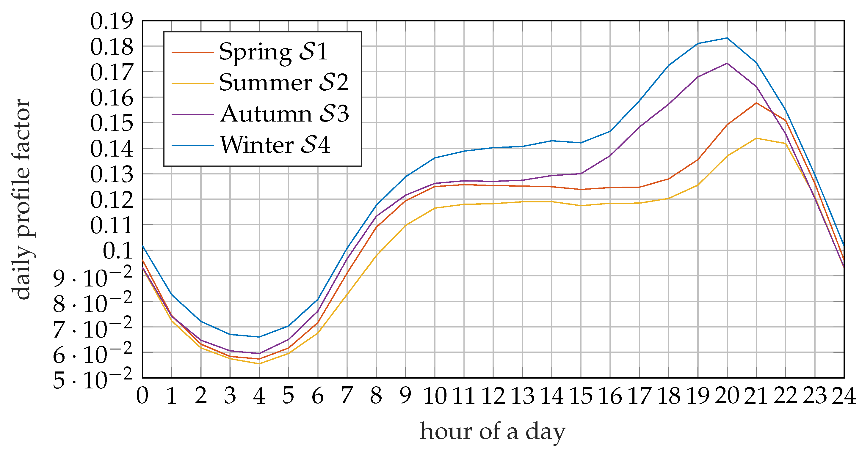
As the subject of analysis in this paper is the daily operating cycle of energy storages, the set of profile factors from the entire year is grouped into 365 daily profiles $w_{d,h}$ for $h\in \left\{1,2,\dots ,24\right\}$ and $d\in \left\{1,2,\dots ,365\right\}$. In order to take into consideration the seasonal changes in the daily load profile, the 365 daily profiles are grouped into 4 seasons according to the season of the year: Spring ($\mathcal{S}1$), Summer ($\mathcal{S}2$), Autumn ($\mathcal{S}3$) and Winter ($\mathcal{S}4$). Then, a reference daily profile was determined for each season of the year as the median of values of individual profile factors with the same hour. For example, for the h-th hour of the reference daily profile in the Spring season $w_h^{\left(S1\right)}$, the value of the profile factor was determined on the basis of the following relationship:

$$w_h^{\left(\mathcal{S}1\right)}=median\left(\left\{w_{d,h}:d\in \mathcal{S}1\right\}\right)$$

(6)

Figure 1 presents the daily load profile for all four seasons.

2.3. Generation Profiles

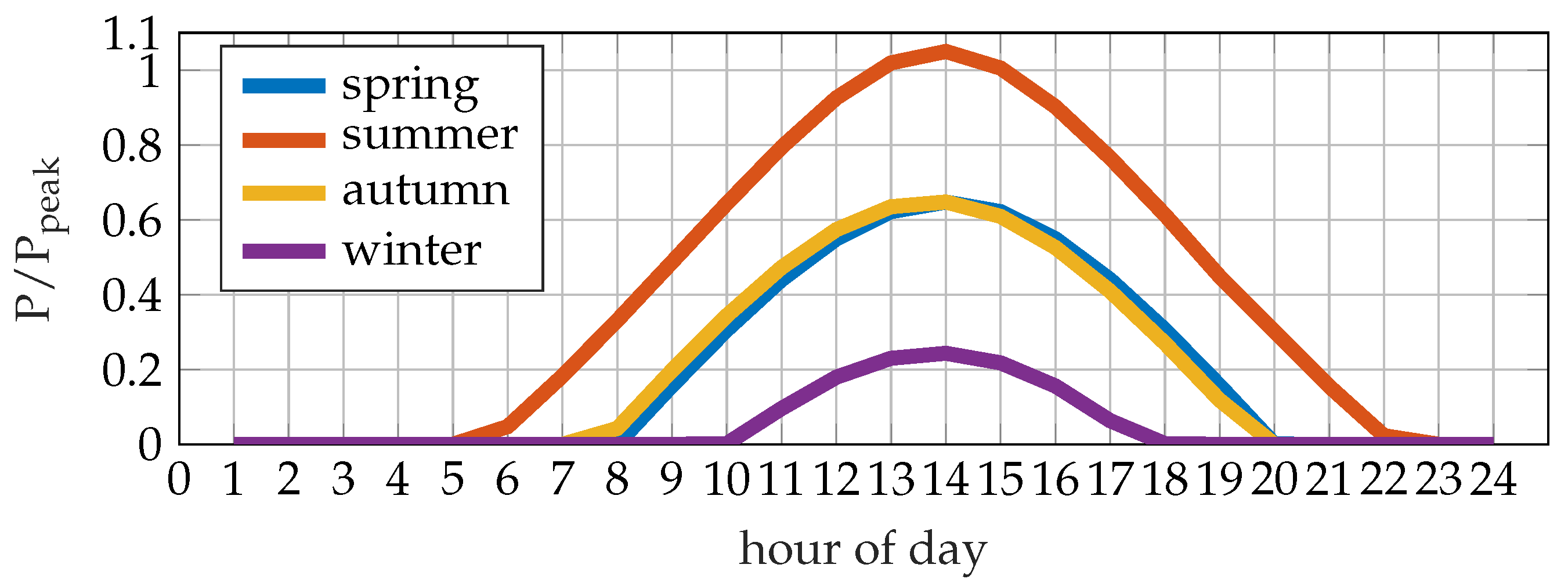
In the power system, in addition to the fully controllable energy sources, there are also RES, for which the electricity production profile depends on the weather conditions. In this paper, generation from PV sources is analysed. A simplified model based on a variable angle of azimuth for a selected geographical location during the first days of Spring, Summer, Autumn and Winter has been adopted as the daily electricity generation profile. An assumption is made that the highest power is generated in Summer when the sun is at its zenith (105% of installed peak power). At other times and on other days, the generated power varies proportionately to the change in the angle of azimuth. Figure 2 presents the generation profile obtained on the basis of the location of the city of Poznan, in Poland.

2.4. Energy Storage Model

Assuming that the charging or discharging process takes place with a constant power for the time $\Delta t$, the stored energy at the moment $t+\Delta t$ will be equal to [35,36]:

$$E_{BES}(t+\Delta t)=E_{BES}\left(t\right)+P_{BES}·\Delta t$$

(7)

whereby:

$$E_{BES}\in 〈0,E_{max}〉$$

(8)

$$P_{BES}=\left\{\begin{array}{l}{P}_E·{\eta }_{in}\mathrm{when}0\le P_E\le P_{max}\\ P_E/{\eta }_{out}\mathrm{when}-P_{max}\le P_E<0\end{array}\right.$$

(9)

$$\left|P_{BES}(t+\Delta t)-P_{BES}\left(t\right)\right|\le \Delta P_{max}$$

(10)

where: $E_{BES}$—energy stored in an energy storage, $P_{BES}$—storage charging (>0) or discharging (<0) power, $P_E$—electric power supplied or drawn from the power system to BESS, ${\eta }_{in},{\eta }_{out}$—efficiency of the charging and discharging process, respectively, $\Delta P_{max}$—maximum power variation $P_{BES}$ resulting from technological limitations, at $\Delta t$.

In accordance with relationship (7), in order to determine the currently stored energy, it is necessary to know its value before starting the charging process. The measure of filling the energy storage with energy is the State of Charge (SOC) described by the following relationship [35]:

$$SOC=\frac{E_{BES}}{E_{max}}\wedge SOC\in 〈0,1〉$$

(11)

During the charging process, BESS draws electricity from the power system and returns it during the discharging process. Therefore, Equation 1 can be written in a modified form for the charging process:

$$P_{Gi}=P_{Di}+\sum _{j=1}^N{V}_i{V}_j(G_{ij}cos\left({\theta }_{ij}\right)+B_{ij}sin\left({\theta }_{ij}\right))+\frac{P_{BES}}{{\eta }_{in}}$$

(12)

and discharging process:

$$P_{Gi}=P_{Di}+\sum _{j=1}^N{V}_i{V}_j(G_{ij}cos\left({\theta }_{ij}\right)+B_{ij}sin\left({\theta }_{ij}\right))+P_{BES}·{\eta }_{out}$$

(13)

An assumption has been made in our study that a lithium-ion energy storage is used. It may be discharged until $SOC=0.2$, and this is the state of charge of the energy storage at the beginning of the day. It has been assumed that the shortest discharge time of the energy storage from $SOC=1$ to $SOC=0.2$ is 1 h. Hence, the highest power $P_{max}$ which discharges the BESS may be determined on the basis of its capacity as:

$$P_{max}=0.8·E_{max}/1\mathrm{h}$$

(14)

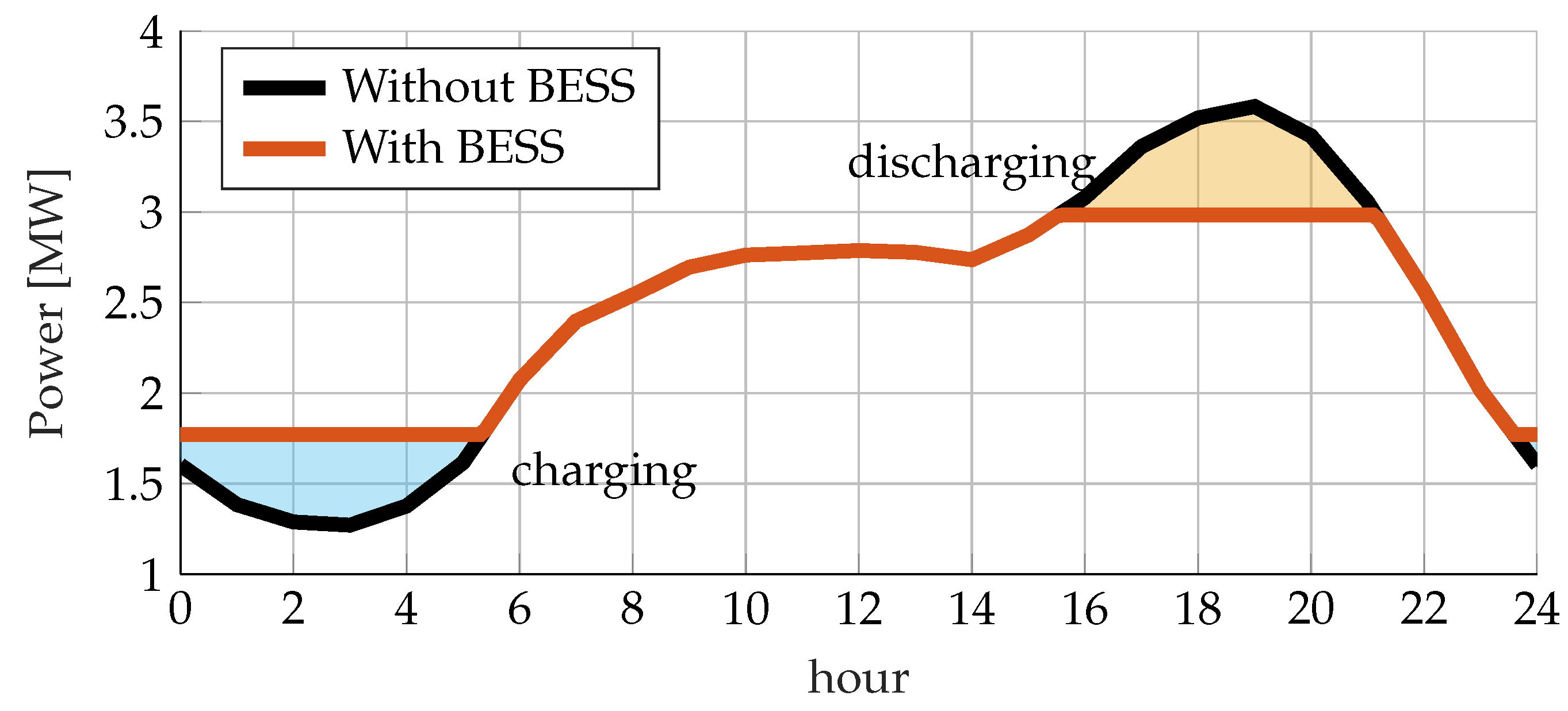
In the case under analysis, the energy storages are supposed to perform the task of reducing transmission losses. The highest daily losses occur during peak hours when the network load is the highest. In order to reduce them, an assumption has been made that storages operate using the Peak Shaving strategy. One of the assumptions for the control algorithm is that the energy returned to and drawn from the energy storage is the same after the full daily cycle. This way, the continued availability of the BESS is ensured.

Figure 3 presents the principle of operation of the peak shaving strategy. The partition levels at which the BESS charging and discharging processes take place are selected in such a way as to make full use of the capacity of the energy storage. Here, this is done using the known daily power waveform. In practice, predictive and optimisation methods [37,38], which are not covered by the scope of this paper, are used to determine the appropriate levels.

2.5. Multiobjective Problem Formulation

The optimisation problem presented in this article is the location of energy storages and the determination of their capacity in the branched distribution system with the connected conventional and PV sources. The storages which operate following the peak shaving strategy are supposed to reduce power losses in the analysed distribution network. Mathematically, the optimisation problem may be presented as a search for vector ${\mathbf{E}}_{\mathbf{max}}=\left\{E_{max,i}\right\}$ of the BESS capacity, which ensures the minimisation of losses in system lines (objective 1), determined by the following relationship:

$$f_1\left({\mathbf{E}}_{\mathbf{max}}\right)=Y·\frac{365}{4}\sum _{h=1}^{24}\left(P_{loss,h}^{\left({\mathcal{S}}_1\right)}+P_{loss,h}^{\left({\mathcal{S}}_2\right)}+P_{loss,h}^{\left({\mathcal{S}}_3\right)}+P_{loss,h}^{\left({\mathcal{S}}_4\right)}\right)$$

(15)

and the total capacity of the storage (objective 2):

$$f_2\left({\mathbf{E}}_{\mathbf{max}}\right)=\sum _i{E}_{max,i}$$

(16)

whereby:

$$0\le E_{max,i}\le E_{maxcap},i\in {\mathcal{B}}_{BESS}$$

(17)

where: Y—period of analysis, h—time of day, $P_{loss,h}^{\left({\mathcal{S}}_{1-4}\right)}$— power losses described by relationship (3) determined for the reference day of the respective season: ${\mathcal{S}}_1$,${\mathcal{S}}_2$,${\mathcal{S}}_3$,${\mathcal{S}}_4$,$E_{max,i}$—BESS capacity in the i-th system bus, ${\mathcal{B}}_{BESS}$—set of bus numbers where the possibility of the BESS installation is assumed.

3. Multiobjective Optimization Methods

3.1. Pareto and Box Domination

In the task of optimisation of a multi-objective problem, which comprises two or more objectives that contradict each other, as opposed to the single-objective case, there is no possibility of determining the absolute best solution. The improvement of results obtained for one assessment objective causes the values of others to deteriorate. Therefore, in a multi-objective optimisation problem with K objectives, so-called non-dominated solutions are sought. Solution ${\mathbf{x}}_1$ dominates over ${\mathbf{x}}_2$ (we mark it as ${\mathbf{x}}_1\succ {\mathbf{x}}_2)$) if [39]:

$${\mathbf{x}}_1\succ {\mathbf{x}}_2\iff \left(\left(\forall k\in K\Rightarrow f_k\left({\mathbf{x}}_1\right)⊵f_k\left({\mathbf{x}}_2\right)\right)\wedge \left(\exists k\in K\Rightarrow f_k\left({\mathbf{x}}_1\right)⊳f_k\left({\mathbf{x}}_2\right)\right)\right)$$

(18)

where: $f_k\left({\mathbf{x}}_1\right)⊵f_k\left({\mathbf{x}}_2\right)$—means that solution ${\mathbf{x}}_1$ is no worse than solution ${\mathbf{x}}_2$ for the k-th objective, and $f_k\left({\mathbf{x}}_1\right)⊳f_k\left({\mathbf{x}}_2\right)$—means that solution ${\mathbf{x}}_1$ is better than solution ${\mathbf{x}}_2$ for the k-th objective (lower for minimisation and higher for maximisation). The set of non-dominated solutions in the K dimensional objective space creates the so called Pareto front.

The authors used the evolutionary methods of multi-objective optimisation in the paper to search for the Pareto front. These methods simultaneously process a set of multiple solutions (so-called populations). Each solution is represented as the so-called individual, which has its own chromosome built of genes (encoded values of decision variables). Individuals in a population are subject to processes modelled on the theory of evolution: crossover, mutation and selection. The role of crossover is to mix the respective solutions (so-called parents) with each other and the result of this is the creation of completely new solutions (so-called offspring). Mutation is the process of random change in the value of selected genes of an individual. On the other hand, selection allows for the selection of the best individuals from the entire population based on their adaptation [40].

During its operation, the evolutionary method should be characterised by high convergence to the actual Pareto front (this is an important condition especially when the calculation of the value of criteria is time-consuming) and ensure the appropriate spread of points on the front (diversity of solutions). In many cases, the excessive number of non-dominated points means that the uniform distribution of points on the currently found front becomes the main goal of the optimisation algorithm. In such a situation, a local and not global front is found.

One of the methods which allow for an increase in the distribution of solutions for simultaneous maintenance of convergence to the global solution is the use of the $ϵ$-dominance described in [40]. It consists of the division of the objectives pace into smaller K-dimensional areas (in the case of the two-objective optimisation, these will be rectangles) to which the discovered $\mathbf{x}$ solutions are assigned. Each area has its own index $I\in {\mathbb{R}}^K$, whose coordinates increase in accordance with the values of objectives that correspond to them. If the ${\mathbf{x}}_1$ and ${\mathbf{x}}_2$ solutions lie in different areas, that is [40]:

$$\exists k\in K\Rightarrow I\left({\mathbf{x}}_1\right)\ne I_k\left({\mathbf{x}}_2\right)$$

(19)

then the condition of dominance of ${\mathbf{x}}_1$ over ${\mathbf{x}}_1$ can be presented as [40]:

$${\mathbf{x}}_1\succ {\mathbf{x}}_2\iff \left(\left(\forall k\in K\Rightarrow I_k\left({\mathbf{x}}_1\right)⊵I_k\left({\mathbf{x}}_2\right)\right)\wedge \left(\exists k\in K\Rightarrow I_k\left({\mathbf{x}}_1\right)⊳I_k\left({\mathbf{x}}_2\right)\right)\right)$$

(20)

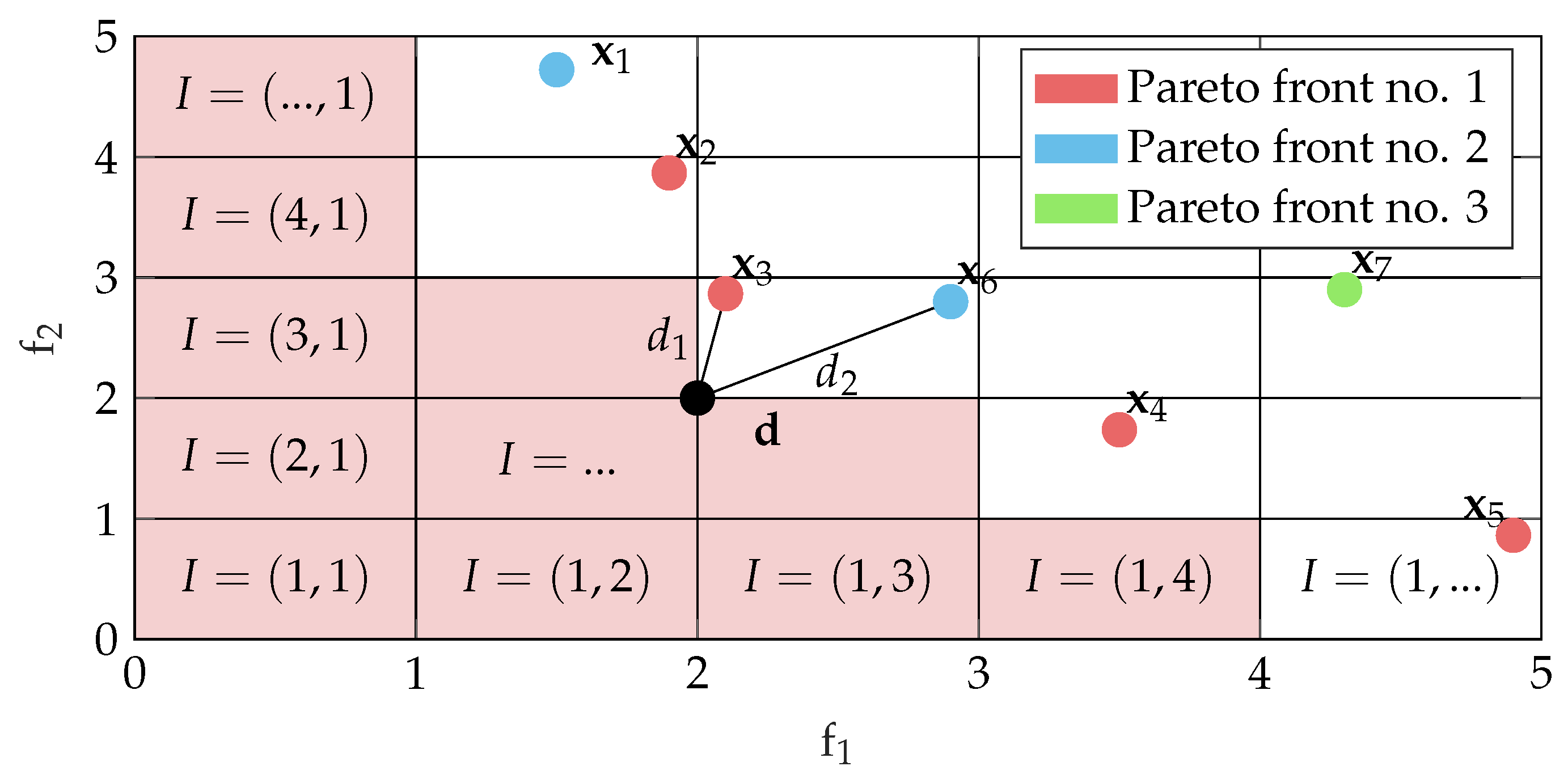
When both solutions lie in the same area (condition (19) is not fulfilled), the dominance is determined on the basis of the distance of both solutions from corner $\mathbf{d}$ which determines the best solution to be obtained in the given area. Hence [40]:

$${\mathbf{x}}_1\succ {\mathbf{x}}_2\iff ∥{\mathbf{x}}_1-\mathbf{d}∥<∥{\mathbf{x}}_2-\mathbf{d}∥$$

(21)

Figure 4 presents an example of analysis of dominance of a group of solutions to a bi-objective problem in accordance with the definition of the $ϵ$-box dominance.

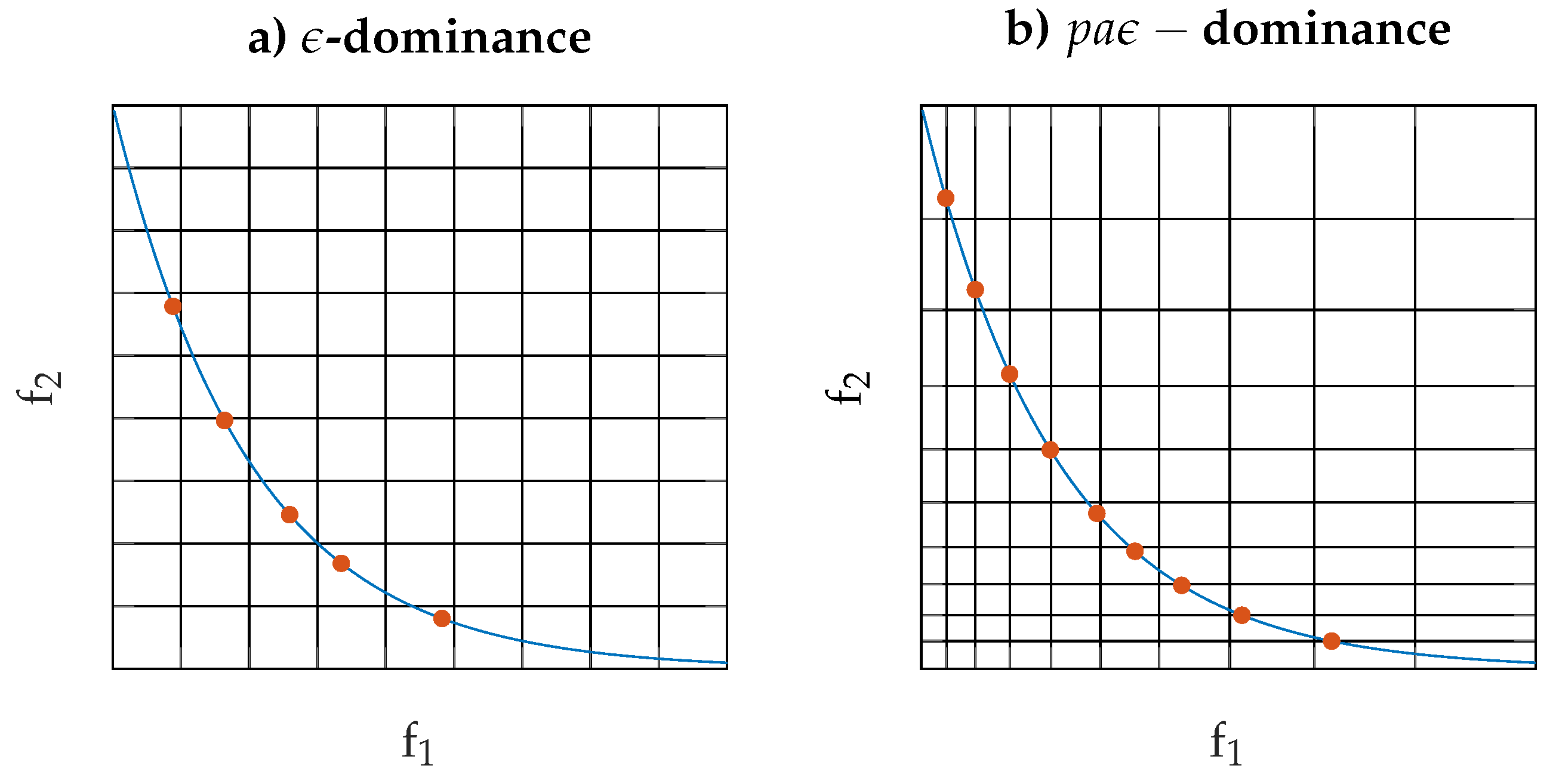
It was noticed in a paper by [41] that division into equal sub-spaces may entail the loss of extreme points. Additionally, the uniformity of the solutions found depends on the shape of the front (its convexity). Therefore, an adaptive division of the objective space ($paϵ$-dominance) was proposed, in which the division grid is condensed at the extremities of the currently found front and expanded in the middle range, based on an analysis of the convexity of the front.

Figure 5 presents the comparison of the grid created in accordance with the $ϵ$-dominance and $paϵ$-dominance. As can be seen, for the $paϵ$-dominance, the grid is condensed, therefore the non-dominated points are distributed more uniformly along the entire front and there are more of them at its extremities.

3.2. NSGA-II

NSGA-II was assumed as a reference evolutionary method. It is described in detail in [42]. The method is characterised by fast non-dominated sorting, a procedure for estimating solution congestion and operator of its comparison [43]. In each iteration, a temporary population $R_t$ is formed. It comprises: the N-element, population $P_t$, and the offspring population $Q_t$ of the same size, which is a result of the use of genetic operators. In accordance with the adopted definition of dominance, each individual is assigned the number of the front on which the individual is located. The first front is composed of non-dominated individuals in the overall population. The second front includes individuals dominated only by individuals from the first front and not dominated by the remaining part of the population, etc. All the individuals are then sorted in an ascending order based on the number of the front. A congestion distance is set for each individual. That distance determines how close a given individual is to the neighbouring individuals from the same front. Based on the number of the front and the congestion distance, the N individuals are selected from $R_t$ to form a new population $P_{t+1}$.

3.3. BRKGA

The BRKGA method presented in [44] is a modification of the RKGA method described in [45]. It was designed to solve multi-objective combinatorial problems. One of the characteristics of this method is the transformation of decision variables into the form of so-called random keys, with values from the $〈0,1〉$ range. In order to make the determination of the phenotype possible, it is thus necessary to additionally introduce an encoder and decoder, which allow for the transformation of values of decision variables into random keys and vice versa.

In the first phase, N of encoded individuals of population $P_t$ are divided into non-dominated individuals ${\overline{P}}_e$ and dominated individuals ${\overline{P}}_e$. Then, pairs of parents are drawn. First, individual a from $P_e$ is drawn. Then, one dominated individual b from $Pe$ is drawn to the pair. The pair of individuals a and b is subject to crossover according to the coin tossing method. For each of the k genes, a random number is drawn from the $〈0,1〉$ range (coin tossing), which determines whether a newly formed offspring will have the gene of individual a or b. Whereby, the likelihood of adopting the trait of parent a (${\rho }_a$) should be higher than in the case of individual b (${\rho }_b=1-{\rho }_a$). In the source paper, the proposed value ${\rho }_a=0.75$ is adopted.

Table 1. Example of a crossover of two parents a and b using the coin tossing method. Individuals have 4-gene chromosomes. After generating 4 random numbers (one per each gene), the obtained values are compared to ${\rho }_a$.

Item	Gene 1	Gene 2	Gene 3	Gene 4
Parent a	0.52	0.8	0.43	0.3
Parent b	0.74	0.34	0.54	0.26
Random	0.62	0.45	0.81	0.35
${\rho }_a=0.75$	<	<	>	<
Offspring	0.52	0.8	0.54	0.3

presents an example of a crossover of chromosomes with 4 genes.

In the selection process, an elitist strategy is used, which involves transferring a certain number of individuals from group $P_e$ to a new population. Then, the group is joined by the offspring obtained as a result of crossover. Finally, the new generation is supplemented by randomly generated individuals so that the size of the population is always constant.

3.4. MPSO

In the case of the PSO algorithm, instead of creating new offspring based on genetic operators, individuals belonging to the given population perform a random move in the space of the decision variables. The direction and length of movement are influenced by three components: inertia (the value of the previous step taken by the individual), the cognitive component (which depends on the best position the individual has been in so far) and the social component (which depends on the globally best solution). The MPSO, which is described in detail in the paper by [46], was used in the tests.

4. Test Case and Results

4.1. Cases Description

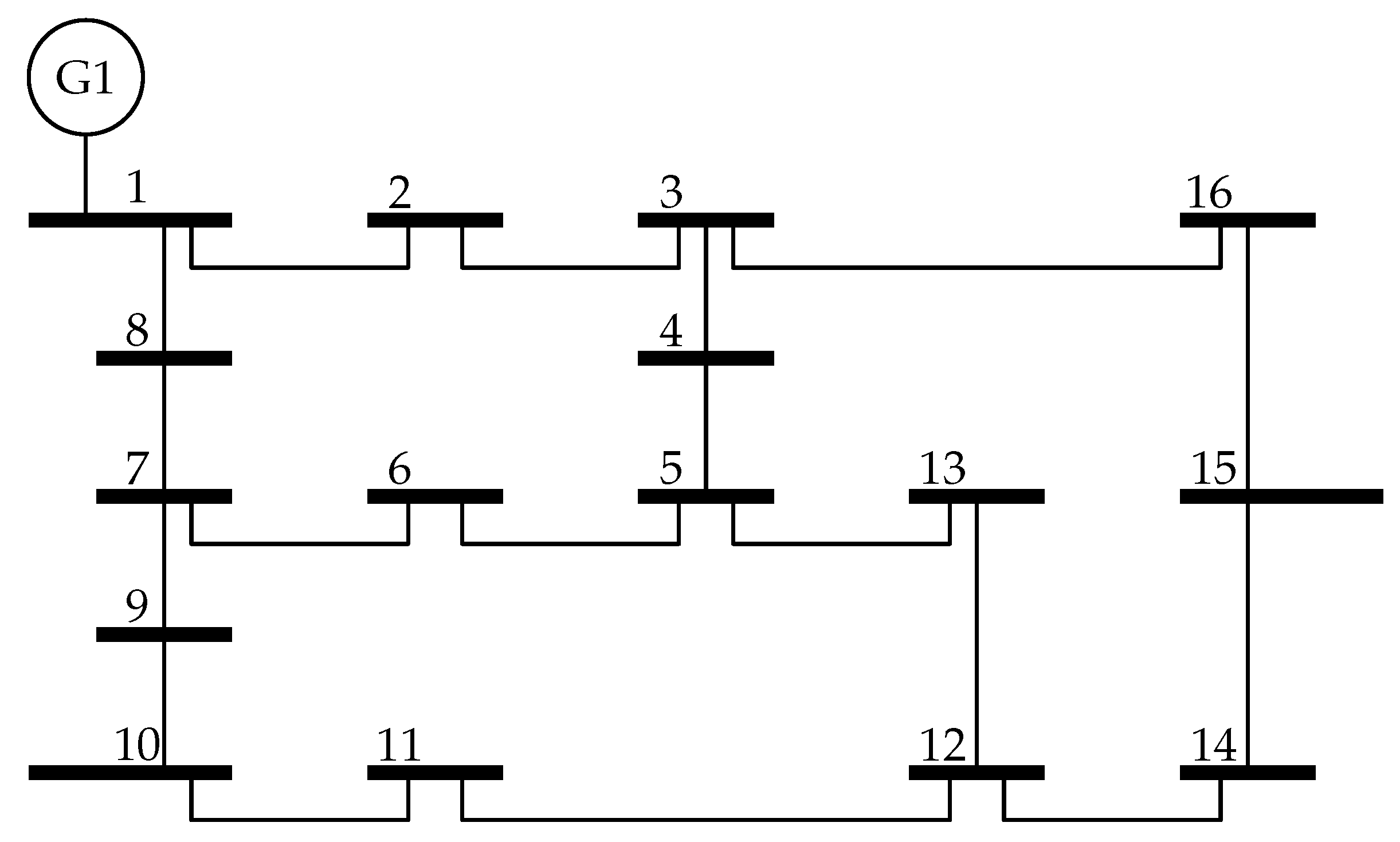
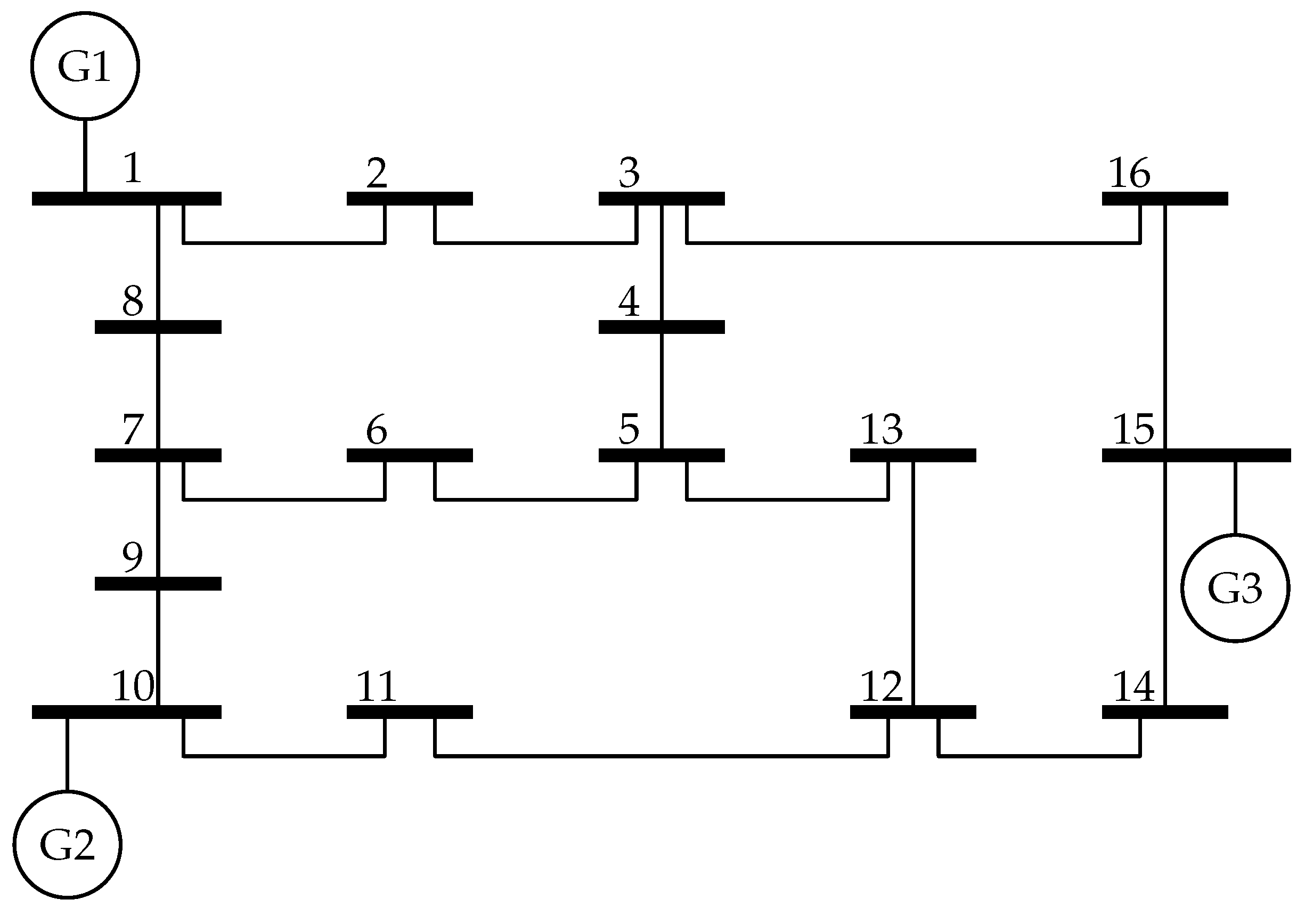
Tests involving the search for the locations of energy storages and their capacities was carried out on a 16-bus medium voltage distribution system in a mixed configuration. The vector of decision variables consist of 16 integers. Each variable corresponds to capacity of Energy Storage (with selected resolution of 100 kWh) installed in one of 16 system buses. The structure of the system is presented in Figure 6. The basic source of power supply is the conventional generator G1 connected to the network feeder with a maximum power of 1000 MW. This is the case of a classic reactive distribution system.

Table 2. List of load values for the respective system buses.

Bus No.	P [MW]	Q [MVar]	Bus No.	P [MW]	Q [MVar]
1	0	0	9	35	26.9
2	50	30.2	10	0	0
3	35	7.7	11	35	16.4
4	40	21.8	12	30	5.4
5	45	23.6	13	25	15
6	40	5.2	14	35	7.1
7	35	3.3	15	0	0
8	50	19.9	16	35	19.6
Overall				490	202.1

presents the load of system buses taken as annual average values. On their basis, reference load profiles were determined in accordance with the methodology described in Section 2.2.

The paper analyses four test cases for which energy storage locations and capacities were sought to reduce power losses in the distribution system lines. The cases differ in terms of the location of RES (PV) with a total power of 50 MW. Nodes 10 and 15 were selected as connection points for PV sources. They ensure a great distance between all the working generations. For the purposes of optimisation, an assumption was made that the maximum capacity of an energy storage in a single bus must not be higher than 100 MWh, and the capacity is determined with an accuracy of 100 kWh. Energy losses in system lines were determined with an assumption that the energy storage would operate for a period of 10 years. This is the standard period of use of energy storages that use lithium-ion cells.

4.1.1. System without RES—Test Case 1

In the base case, in which it was assumed that there are no directly connected renewable sources in the analysed system. The only generator is generator G1.

4.1.2. System with PV Generation at Bus 10—Test Case 2

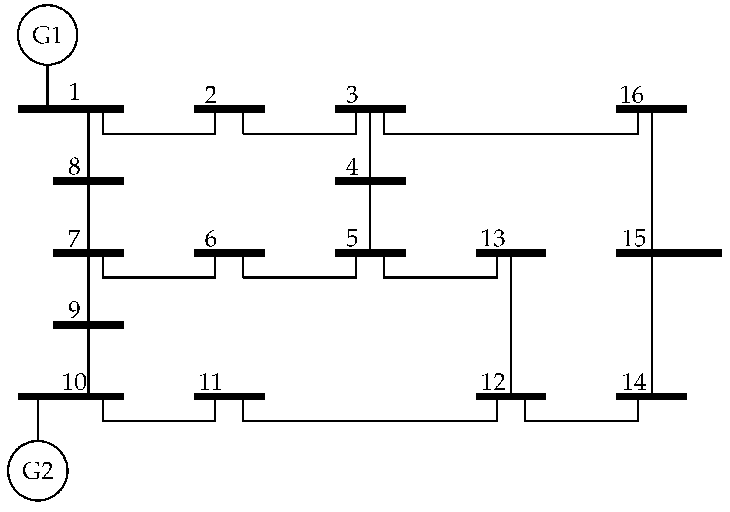
For the system described in Case 2, in addition to generator G1, a 50 MW PV generation was added in bus 10 as per Figure 7. The generation profile was created on the basis of information included in Section 2.3.

4.1.3. System with PV Generation at Bus 15—Test Case 3

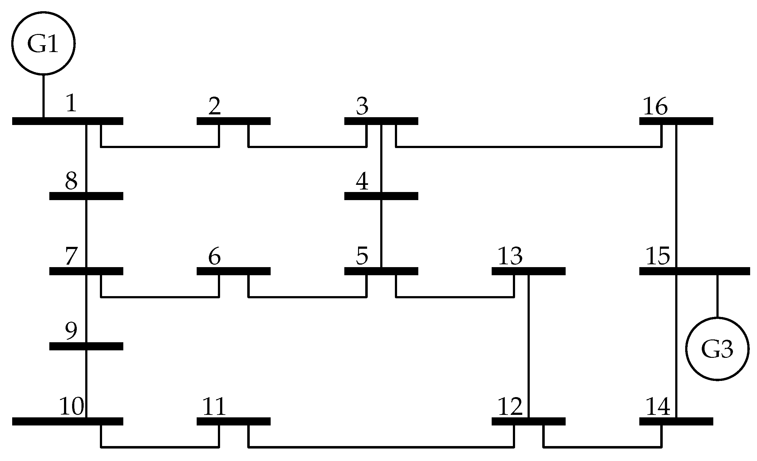
In another variant for the system from Case 1,a PV generation with a peak power of 50 MW was added in bus 15. Figure 8 presents the analysed case of the system.

4.1.4. System with Two PV Generations—Test Case 4

In the last analysed variant for the system from Case 1, two PV generators, in buses 10 and 15, were added. The peak power of both generators is 25 MW, and their total PV generator power is equal to the one used in Case 2 and Case 3. Figure 9 presents the analysed case of the system.

4.2. Results

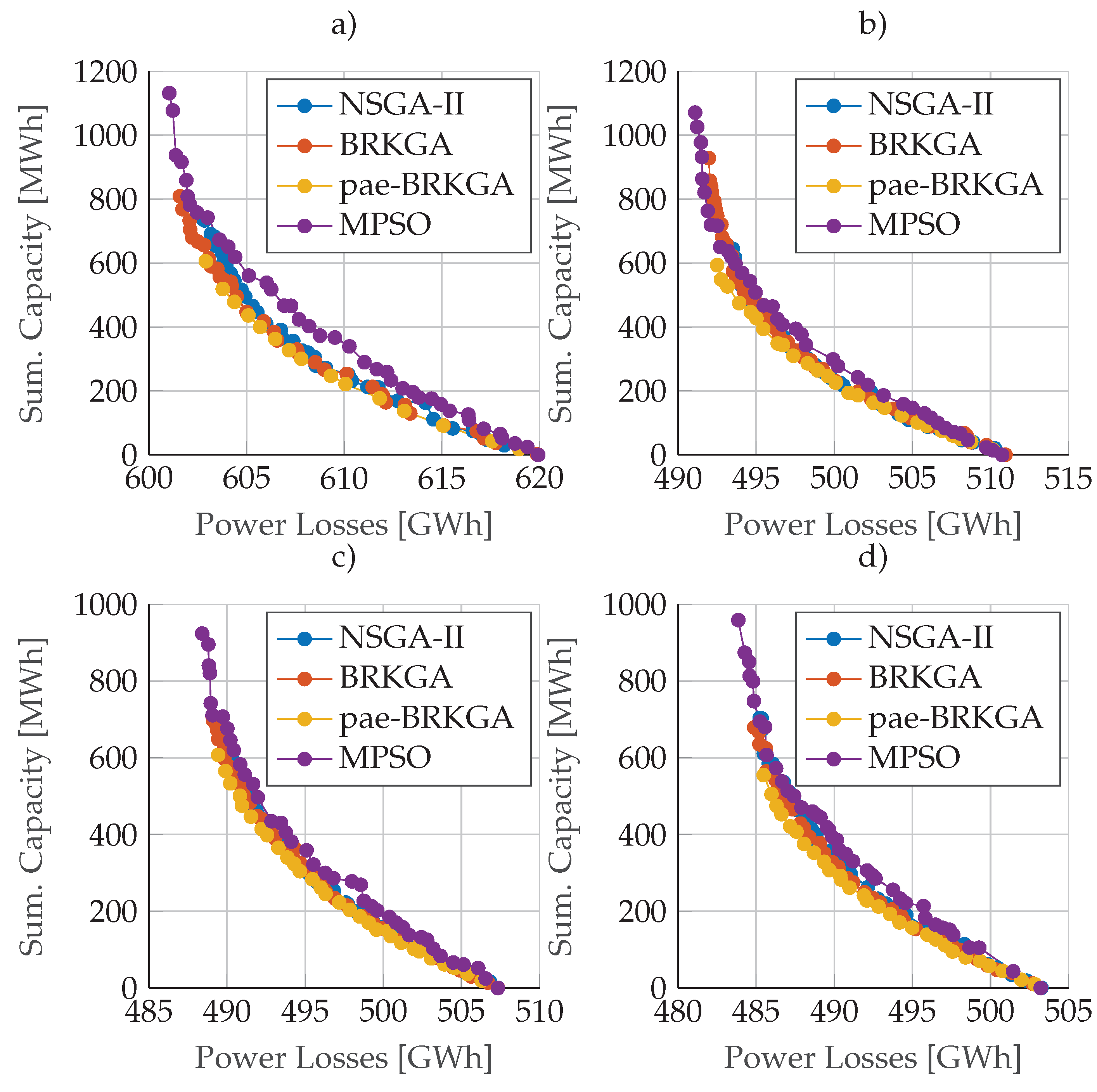
Figure 10 presents the Pareto fronts determined using the NSGA-II, MPSO and BRKGA methods. For the BRKGA method, also $paϵ$-dominance ($paϵ-$BRKGA) was used.

In order to determine the quality of the solutions obtained through the used optimisation methods, all the found non-dominated solutions were collected into single set $X:\mathrm{method}\mathrm{name},f_1,f_2$. Then, on the basis of the values of objectives $f_1$ and $f_2$ from X, all solutions not dominated by the other ones were selected (in accordance with Equation 18). For each method, the relative efficiency $\eta$ by the authors was determined:

$$\eta =\frac{N_{nond}}{N_{all}}·100\%$$

(22)

where: $N_{nond}$—number of non-dominated solutions determined by means of the analysed method, which were not dominated by the other solutions from set X, $N_{all}$—number of all solutions from set X, which were found by the analysed method. This way, the quality of solutions found with one method will be determined in relation to the others. If $\eta =100\%$, then this means that the whole front found by the method is not worse than the solutions found by a different method. The lower the efficiency, the lower the percentage of solutions of a given method is in the actual Pareto front (their quality is worse).

Table 3. Methods Efficiency for different test cases.

Case	Method Efficiency $\mathit{\eta }$ (Founded Solutions ${\mathit{N}}_{\mathbf{all}}$)
	NSGA-II	BRKGA	$\mathbf{pa}\mathit{ϵ}$-BRKGA	MPSO
Test Case 1	29% (38)	62% (37)	100% (17)	12% (41)
Test Case 2	53% (38)	37% (41)	96% (24)	32% (41)
Test Case 3	27% (41)	41% (41)	94% (35)	17%(41)
Test Case 4	8% (37)	34% (41)	79% (39)	20% (41)

lists the efficiency of the NSGA-II, BRKGA and $paϵ-$BRKGA methods, obtained in the respective test cases. In each test case, the efficiency of the $paϵ-$BRKGA method is higher than the efficiency of the BRKGA and NSGA-II methods, which means that the majority of solutions found by it is better than the solutions found by the other methods. In the case of the system without RES, the efficiency was 100%, which means that none of the solutions found by $paϵ-$BRKGA is dominated by the solutions of other methods. Attention must be paid to the fact that the inclusion of the RES in a single bus resulted in a slight deterioration in the efficiency of the methods. The lowest efficiency was obtained for test case 4.

A detailed analysis of the found proposals for the location of energy storages was performed for solutions provided by the $paϵ$-BRKGA method, which achieved the highest efficiency. Three solutions were selected in each case, for which the total installed BESS capacity is as close as possible to the following values: 100, 200 and 500 MWh. For each case, an indicator that defines the reduction in energy loss was determined as $\Delta E$:

$$\Delta E=f_{noBESS}-f_1\left({\mathbf{E}}_{max}\right)$$

(23)

where: $f_{noBESS}$—losses in the system without applying BESS ($f_{noBESS}=f_1\left(\mathbf{0}\right)$), ${\mathbf{E}}_{max}$—vector of energy storage capacity for the analysed task.

In order to determine the impact of an energy storage on the reduction of power losses, the index referred to as efficiency $\Psi$ of the BESS installation defined as:

$$\Psi =\frac{\Delta E}{f_2}$$

(24)

The list of the locations of energy storages and their capacities in the respective system buses, the total capacity (objective $f_2$), loss reduction ($\Delta E$) and efficiency of the BESS installation ($\Psi$) are presented in:

Table 4. Three solutions founded by $paϵ$-BRKGA with ca. 100 MWh, 200 MWh and 500 MWh of overall BESS capacity for Test Case 1.

Bus No.	ca. 100 MWh [MWh]	ca. 200 MWh [MWh]	ca. 500 MWh [MWh]
1	0.0	0.0	0.0
2	0.2	0.2	42.4
3	0.2	0.2	36.6
4	0.2	0.2	74.4
5	0.3	85.1	85.1
6	0.0	0.0	80.2
7	1.5	1.5	0.0
8	0.0	0.0	0.0
9	0.0	0.0	0.0
10	0.0	0.0	0.0
11	0.0	0.0	40.3
12	38.9	38.9	38.9
13	49.1	49.1	49.1
14	0.2	45.3	70.8
15	0.0	0.2	0.0
16	0.9	0.9	0.9
${\mathbf{f}}_{\mathbf{1}}$[MWh]	91.5	221.6	518.7
$\mathbf{\Delta }\mathbf{E}$[MWh]	5855.2	11,856.7	19,405.6
$\mathsf{\Psi }$[MWh/MWh]	64.0	53.5	37.4

for Case 1,

Table 5. Three solutions founded by $paϵ$-BRKGA with ca. 100 MWh, 200 MWh and 500 MWh of overall BESS capacity for Test Case 2.

Bus No.	ca. 100 MWh [MWh]	ca. 200 MWh [MWh]	ca. 500 MWh [MWh]
1	0.0	0.0	0.0
2	0.0	0.0	0.0
3	0.0	0.0	0.0
4	0.1	0.1	80.5
5	0.2	48.9	88.1
6	10.5	15.7	94.6
7	0.0	0.1	0.1
8	0.1	0.0	0.1
9	0.0	0.0	0.0
10	0.3	0.3	0.3
11	0.1	39.0	39.0
12	31.4	31.4	29.1
13	58.2	58.2	58.2
14	0.1	0.1	84.2
15	0.0	0.0	0.0
16	0.2	0.2	0.2
${\mathbf{f}}_{\mathbf{1}}$[MWh]	101.2	194.0	474.4
$\mathbf{\Delta }\mathbf{E}$[MWh]	6993.3	12,292.5	20,697.8
$\mathsf{\Psi }$[MWh/MWh]	69.1	63.4	43.6

for Case 2,

Table 6. Three solutions founded by $paϵ$-BRKGA with ca. 100 MWh, 200 MWh and 500 MWh of overall BESS capacity for Test Case 3.

Bus No.	ca. 100 MWh [MWh]	ca. 200 MWh [MWh]	ca. 500 MWh [MWh]
1	0.1	0.1	0.1
2	0.0	0.1	0.3
3	0.0	0.0	0.0
4	0.0	0.0	65.5
5	59.0	59.0	78.4
6	0.2	0.0	94.5
7	0.1	9.8	0.1
8	0.2	0.2	0.2
9	0.0	0.2	0.2
10	0.0	0.0	0.0
11	0.2	34.1	49.7
12	40.3	40.3	40.3
13	0.2	58.8	58.8
14	0.3	0.1	86.7
15	0.0	0.2	0.0
16	0.0	0.2	0.2
${\mathbf{f}}_{\mathbf{1}}$[MWh]	100.6	203.1	475.0
$\mathbf{\Delta }\mathbf{E}$[MWh]	6614.9	11,601.8	19,910.1
$\mathsf{\Psi }$[MWh/MWh]	65.8	57.1	41.9

for Case 3 and

Table 7. Three solutions founded by $paϵ$-BRKGA with ca. 100 MWh, 200 MWh and 500 MWh of overall BESS capacity for Test Case 4.

Bus No.	ca. 100 MWh [MWh]	ca. 200 MWh [MWh]	ca. 500 MWh [MWh]
1	0.0	0.0	0.0
2	0.1	0.1	0.1
3	0.0	0.0	36.7
4	0.1	0.2	72.0
5	0.0	87.3	87.3
6	0.1	0.1	66.0
7	0.1	0.1	22.0
8	0.1	0.1	40.9
9	0.0	0.1	0.0
10	0.1	0.1	0.0
11	33.0	42.9	42.9
12	0.1	0.1	45.6
13	45.9	45.9	45.9
14	15.3	15.3	15.3
15	0.0	0.1	0.0
16	0.1	0.2	0.0
${\mathbf{f}}_{\mathbf{1}}$[MWh]	95.0	192.6	474.7
$\mathbf{\Delta }\mathbf{E}$[MWh]	6800.1	11,772.0	20,497.6
$\mathsf{\Psi }$[MWh/MWh]	71.6	61.1	43.2

for Case 4. The green colour was used to mark energy storages with a capacity higher than 1 MWh. An analysis that was not presented in the article demonstrated that the omission of other energy storage increases power losses within a range between several per mille and approx. 4%, depending on the case under consideration.

In test case 1, when the predicted total capacity of the energy storage is approximately 10 MWh, the largest energy storages are located in buses 12 and 13. These are the buses that are most distant from the network feeder. For 200 MWh installations, large energy storages were additionally complemented by buses 5 (85 MWh) and 14 (45 MWh). These are the buses that are located in the direct vicinity of buses 12 and 13. Attention must be paid to the fact that the energy storage at bus 5 has double the capacity as the other large storages. This is a central bus common for all 3 meshes in the analysed grid. In the case of the third system (ca. 500 MWh), the capacity was increased at bus 14, and new energy storages were located at buses neighbouring with those previously mentioned (5, 12, 13 and 14).

In test cases 2 and 3, where uncontrollable RES were additionally included in the system, just as in test case 1, the solutions for 100 MWh and 200 MWh installations are located between buses 5, 12 and 13. For the installation with a total capacity of approx. 500 MWh, they are distributed on branches that are common for the two meshes of the circuit. In the case of RES connected to bus 10, capacities larger than for Test Case 3 are installed at buses 4 and 14 (they are further away from generator G2). Similarly, for Test Case 3, larger capacities are installed at buses 7 and 11.

In Test Case 4 with two RES included in the system, as a priority larger energy storages are installed at buses 11, 13 and 14. For installations of approximately 200 MWh, an additional BESS is installed at central bus 5, and for 500 MWh installations, the storages are located in the central part of the circuit.

For Test Case 1, on a scale of 10 years of BESS operation, energy losses can be reduced ($\Delta E$) by: approximately 6 GWh for 100 MWh BESS, approximately 12 GWh for 200 MWh BESS and approximately 20 GW for 500 MWh BESS.

In other analysed cases, attention must be paid to the fact that just the presence of RES in the system causes a reduction in energy losses. Owing to this, the energy loss reduction at such a level as in case 1 is possible at a lower total capacity of the energy storage. Hence, for cases 2 and 3, with a single RES supply point, the efficiency $\Psi$ is higher than in case 1. For case 4, where there are three supply points, distributed generation from the two RES means that the BESS located in the system can be recharged from a source that is closer, so losses during the off-peak BESS recharging process are reduced. Owing to this, the achieved values of $\Psi$ were, relatively, the highest in case 4.

5. Conclusions

The paper has demonstrated that evolutionary multi-objective optimisation methods are an effective tool in determining the location of BESS in the power system to minimise transmission losses. This has been demonstrated by way of solving a multi-objective and integer problem of BESS location in four variants of a mixed medium voltage distribution system - with classic and renewable PV generations.

As part of the study, three optimisation methods were compared - NSGA-II, BRKGA, MPSO. The procedure for determination of the relative efficiency of the $\eta$ method proposed by the authors allowed for the comparison of results obtained with their application. It has been proven that using the BRKGA method, designed to solve combinatorial problems, gives better results than the widely used and universal NSGA-II and MPSO methods. Additionally, it has been shown that the use of the modified definition of dominance in the Pareto sense, in the form of the so-called $paϵ$-dominance, increases the efficiency of the BRKGA method.

In order to compare the solutions obtained in Pareto fronts, the index $\Psi$ called the efficiency of the BESS installation was introduced. It is defined as the ratio of energy saved, owing to $\Delta E$ included in the BESS installation, to the total capacity of the storage. An increase in the capacity of BESS in the system leads to a decrease in efficiency defined in this way, which means that the larger the capacity of the storages included in the system, the less effect they have on reducing the energy losses. Therefore, optimal selection of the total capacity of energy storages and their location is necessary, depending on the structure of the system, including the presence of BESS in the system. By taking advantage of the optimisation results, it was determined that in each of the test cases solved, a set of buses with the softest potential for power loss reduction was identified. The omission (capacity zeroing) of energy storages in the remaining buses does not lead to a significant increase in transmission losses. Additionally, because of the smaller number of locations of the storages, the costs of BESS operation are limited.

In accordance with the current knowledge, the integration of RES in the form of PV sources into the system under investigation results in a reduction in total power losses when compared to an identical system with conventional generation only. The complementation of the system with energy storages identified by way of optimisation, installed at a certain distance from RES, leads to a further reduction in power transmission losses while maintaining a significantly higher efficiency $\Psi$ than in the case of the reactive distribution system. This means that the more distributed the generation is, the more effective and economically justifiable the use of BESS is.

The multi-objective optimisation method for the determination of the location of energy storages, which has been presented in the paper, is designed for mixed distribution systems. It is possible to use it in radial systems, however, significantly greater calculation resources will be used to determine a solution than in the case of methods dedicated to this type of system (described, e.g., in paper [29]). This state of affairs follows from the fact that the proposed method is based on the multiple determination of power flow. The time in which the result is obtained is greatly affected by the size of the system—in the case of systems containing hundreds or thousands of nodes, it is necessary to apply parallel computing. Analysis of the obtained results indicates that it is possible to determine the relevant nodes for BESS installations (with a high efficiency $\Psi$) and delineate the sequence of their installation. This method, however, does not take into account a full analysis based on the calculations of costs and benefits resulting from the use of the BESS installation.

Despite the significant costs of integrating energy storages into the power system, their installations should not only be viewed through the perspective of reductions in transmission losses. The integration of the energy storages allows for the postponement of or resignation from the upgrading/expansion of the system, a reduction in operating costs, and also often leads to improvements in the quality of the electricity in systems containing intermittent energy sources such as PV. Additionally, in periods of lower energy demand, the installed energy storages may be used for other system purposes such as power reserves or exchange controls on the Energy Market.

As part of further research, the authors of the article plan to include elements of economic analysis in the optimisation process, taking into account the predicted costs of network expansion, the extrapolation of energy prices and the unit costs of BESS throughout the period of operation of the installation. Additionally, the impact of other strategies for BESS control will be investigated, i.e., Voltage Support and the efficiency $\Psi$ of the installation. The authors are also planning to take into consideration an analysis of the impact of BESS on the reliability of the power network. The analysis presented in the paper can also be conducted on other energy storage technologies (e.g., Power 2 Gas).

References

- Wilms, Y.; Fedorovich, S.; Kachalov, N.A. Methods of Reducing Power Losses in Distribution Systems. MATEC Web Conf. 2017, 141, 01050. [Google Scholar] [CrossRef] [Green Version]
- Farahani, V.; Sadeghi, S.H.H.; Askarian Abyaneh, H.; Agah, S.M.M.; Mazlumi, K. Energy Loss Reduction by Conductor Replacement and Capacitor Placement in Distribution Systems. IEEE Trans. Power Syst. 2013, 28, 2077–2085. [Google Scholar] [CrossRef]
- Levitin, G.; Kalyuzhny, A.; Shenkman, A.; Chertkov, M. Optimal Capacitor Allocation in Distribution Systems Using a Genetic Algorithm and a Fast Energy Loss Computation Technique. IEEE Trans. Power Deliv. 2000, 15, 623–628. [Google Scholar] [CrossRef]
- Hooshmand, R.; Ataei, M. Optimal Capacitor Placement in Actual Configuration and Operational Conditions of Distribution System Using RCGA. J. Electr. Eng. 2007, 58, 189–199. [Google Scholar]
- Salis, G.J.; Safigianni, A.S. Long-Term Optimization of Radial Primary Distribution Networks by Conductor Replacements. Int. J. Electr. Power Energy Syst. 1999, 21, 349–355. [Google Scholar] [CrossRef]
- Ćalasan, M.; Konjić, T.; Kecojević, K.; Nikitović, L. Optimal Allocation of Static Var Compensators in Electric Power Systems. Energies 2020, 13, 3219. [Google Scholar] [CrossRef]
- Yuvaraj, T.; Ravi, K.; Devabalaji, K.R. DSTATCOM Allocation in Distribution Networks Considering Load Variations Using Bat Algorithm. Ain Shams Eng. J. 2017, 8, 391–403. [Google Scholar] [CrossRef] [Green Version]
- Helt, P.; Zduńczyk, P. Optymalizacja konfiguracji dla sieci rozdzielczych SN i nN. Zesz. Nauk. Wydz. Elektrotechniki Autom. Politech. Gdan. 2013, Nr 33, 107–110. [Google Scholar]
- Tandon, A.; Saxena, D. A Comparative Analysis of SPSO and BPSO for Power Loss Minimization in Distribution System Using Network Reconfiguration. In Proceedings of the 2014 Innovative Applications of Computational Intelligence on Power, Energy and Controls with Their Impact on Humanity (CIPECH), Ghaziabad, India, 28–29 November 2014; pp. 226–232. [Google Scholar] [CrossRef]
- Fisher, E.B.; O’Neill, R.P.; Ferris, M.C. Optimal Transmission Switching. IEEE Trans. Power Syst. 2008, 23, 1346–1355. [Google Scholar] [CrossRef] [Green Version]
- Salkuti, S.R. Multi-Objective-Based Optimal Transmission Switching and Demand Response for Managing Congestion in Hybrid Power Systems. Int. J. Green Energy 2020, 17, 457–466. [Google Scholar] [CrossRef]
- Tang, J.; Cartes, D.; Baldwin, T. Economic Dispatch with Piecewise Linear Incremental Function and Line Loss. In Proceedings of the 2003 IEEE Power Engineering Society General Meeting (IEEE Cat. No.03CH37491), Toronto, ON, Canada, 13–17 July 2003; Volume 2, pp. 944–947. [Google Scholar] [CrossRef]
- Zhu, J.; Xiong, X.; Lou, S.; Liu, M.; Yin, Z.; Sun, B.; Lin, C. Two Stage Approach for Economic Power Dispatch. In Proceedings of the 2008 IEEE Power and Energy Society General Meeting—Conversion and Delivery of Electrical Energy in the 21st Century, Pittsburgh, PA, USA, 20–24 July 2008; pp. 1–5. [Google Scholar] [CrossRef]
- Saka, M.; Tezcan, S.S.; Eke, I.; Taplamacioglu, M.C. Economic Load Dispatch Using Vortex Search Algorithm. In Proceedings of the 2017 4th International Conference on Electrical and Electronic Engineering (ICEEE), Ankara, Turkey, 8–10 April 2017; pp. 77–81. [Google Scholar] [CrossRef]
- Mikulski, S.; Tomczewski, A. Ocena metod wyznaczania współczynników rozkładu Weibulla w zagadnieniach energetyki wiatrowej. Poznan Univ. Technol. Acad. J. Electr. Eng. Wydaw. Politech. Pozn. 2016, 119–129. Available online: https://sin.put.poznan.pl/publications/details/n45873 (accessed on 26 October 2021).
- Abu-Mouti, F.S.; El-Hawary, M.E. Optimal Distributed Generation Allocation and Sizing in Distribution Systems via Artificial Bee Colony Algorithm. IEEE Trans. Power Deliv. 2011, 26, 2090–2101. [Google Scholar] [CrossRef]
- Prenc, R.; Škrlec, D.; Komen, V. Distributed Generation Allocation Based on Average Daily Load and Power Production Curves. Int. J. Electr. Power Energy Syst. 2013, 53, 612–622. [Google Scholar] [CrossRef]
- Kansal, S.; Sai, B.B.R.; Tyagi, B.; Kumar, V. Optimal Placement of Distributed Generation in Distribution Networks. Int. J. Eng. Sci. Technol. 2011, 3. [Google Scholar] [CrossRef]
- Kumar, S.; Sarita, K.; Vardhan, A.S.S.; Elavarasan, R.M.; Saket, R.K.; Das, N. Reliability Assessment of Wind-Solar PV Integrated Distribution System Using Electrical Loss Minimization Technique. Energies 2020, 13, 5631. [Google Scholar] [CrossRef]
- Chen, Y.C.; Jiang, X.; Dominguez-Garcia, A.D. Impact of Power Generation Uncertainty on Power System Static Performance. In Proceedings of the 2011 North American Power Symposium, Boston, MA, USA, 4–6 August 2011; pp. 1–5. [Google Scholar] [CrossRef]
- Andrychowicz, M. The Impact of Energy Storage along with the Allocation of RES on the Reduction of Energy Costs Using MILP. Energies 2021, 14, 3783. [Google Scholar] [CrossRef]
- Gu, C.; Zhang, Y.; Wang, J.; Li, Q. Joint Planning of Electrical Storage and Gas Storage in Power-Gas Distribution Network Considering High-Penetration Electric Vehicle and Gas Vehicle. Appl. Energy 2021, 301, 117447. [Google Scholar] [CrossRef]
- Wei, Z.; Moon, B.Y.; Joo, Y.H. Smooth Wind Power Fluctuation Based on Battery Energy Storage System for Wind Farm. J. Electr. Eng. Technol. 2014, 9, 2134–2141. [Google Scholar] [CrossRef] [Green Version]
- Liao, J.T.; Chuang, Y.S.; Yang, H.T.; Tsai, M.S. BESS-Sizing Optimization for Solar PV System Integration in Distribution Grid. IFAC-PapersOnLine 2018, 51, 85–90. [Google Scholar] [CrossRef]
- Shi, L.; Fa, L.; Zhu, H.; Shi, J.; Wu, F.; He, W.; Wang, C.; Lee, K.Y.; Lin, K. Photovoltaic Active Power Control Based on BESS Smoothing. IFAC-PapersOnLine 2019, 52, 443–448. [Google Scholar] [CrossRef]
- Figgener, J.; Stenzel, P.; Kairies, K.P.; Linßen, J.; Haberschusz, D.; Wessels, O.; Angenendt, G.; Robinius, M.; Stolten, D.; Sauer, D.U. The Development of Stationary Battery Storage Systems in Germany—A Market Review. J. Energy Storage 2020, 29, 101153. [Google Scholar] [CrossRef]
- Mora, C.A.; Montoya, O.D.; Trujillo, E.R. Mixed-Integer Programming Model for Transmission Network Expansion Planning with Battery Energy Storage Systems (BESS). Energies 2020, 13, 4386. [Google Scholar] [CrossRef]
- Rizwana, J.; Jeevitha, R.; Venkatesh, R.; Parthiban, K.S. Minimization of Fuel Cost in Solving the Power Economic Dispatch Problem Including Transmission Losses by Using Modified Particle Swarm Optimization. In Proceedings of the 2015 IEEE International Conference on Computational Intelligence and Computing Research (ICCIC), Madurai, India, 10–12 December 2015; pp. 1–4. [Google Scholar] [CrossRef]
- Kalkhambkar, V.; Kumar, R.; Bhakar, R. Energy Loss Minimization through Peak Shaving Using Energy Storage. Perspect. Sci. 2016, 8, 162–165. [Google Scholar] [CrossRef] [Green Version]
- Saini, P.; Gidwani, L. An Environmental Based Techno-Economic Assessment for Battery Energy Storage System Allocation in Distribution System Using New Node Voltage Deviation Sensitivity Approach. Int. J. Electr. Power Energy Syst. 2021, 128. [Google Scholar] [CrossRef]
- Sun, Y.; Wu, X.; Wang, J.; Hou, D.; Wang, S. Power Compensation of Network Losses in a Microgrid With BESS by Distributed Consensus Algorithm. IEEE Trans. Syst. Man Cybern.-Syst. 2021, 51, 2091–2100. [Google Scholar] [CrossRef]
- Van Ness, J.E. Iteration Methods for Digital Load Flow Studies. Trans. Am. Inst. Electr. Eng. Part III Power Appar. Syst. 1959, 78, 583–586. [Google Scholar] [CrossRef]
- Tinney, W.; Hart, C. Power Flow Solution by Newton’s Method. IEEE Trans. Power Appar. Syst. 1967, PAS-86, 1449–1460. [Google Scholar] [CrossRef]
- Sauter, P.S.; Braun, C.A.; Kluwe, M.; Hohmann, S. Comparison of the Holomorphic Embedding Load Flow Method with Established Power Flow Algorithms and a New Hybrid Approach. In Proceedings of the 2017 Ninth Annual IEEE Green Technologies Conference (GreenTech), Denver, CO, USA, 29–31 March 2017; pp. 203–210. [Google Scholar] [CrossRef]
- Yan, Z.; Zhang, X.P. General Energy Filters for Power Smoothing, Tracking and Processing Using Energy Storage. IEEE Access 2017, 5, 19373–19382. [Google Scholar] [CrossRef]
- Tomczewski, A. Optymalizacja Struktury Układu Turbina Wiatrowa—Kinetyczny Magazyn Energii. Przegląd Elektrotechniczny 2016, 1, 142–145. [Google Scholar] [CrossRef]
- Chapaloglou, S.; Nesiadis, A.; Iliadis, P.; Atsonios, K.; Nikolopoulos, N.; Grammelis, P.; Yiakopoulos, C.; Antoniadis, I.; Kakaras, E. Smart Energy Management Algorithm for Load Smoothing and Peak Shaving Based on Load Forecasting of an Island’s Power System. Appl. Energy 2019, 238, 627–642. [Google Scholar] [CrossRef]
- Hwang, J.S.; Rosyiana Fitri, I.; Kim, J.S.; Song, H. Optimal ESS Scheduling for Peak Shaving of Building Energy Using Accuracy-Enhanced Load Forecast. Energies 2020, 13, 5633. [Google Scholar] [CrossRef]
- Deb, K. Multi-Objective Optimization Using Evolutionary Algorithms, 1st ed.; Wiley-Interscience Series in Systems and Optimization; John Wiley & Sons: Chichester, NY, USA, 2001. [Google Scholar]
- Deb, K.; Mohan, M.; Mishra, S. Evaluating the E-Domination Based Multi-Objective Evolutionary Algorithm for a Quick Computation of Pareto-Optimal Solutions. Evol. Comput. 2005, 13, 501–525. [Google Scholar] [CrossRef] [PubMed]
- Hernández-Díaz, A.G.; Santana-Quintero, L.V.; Coello Coello, C.A.; Molina, J. Pareto-Adaptive e-Dominance. Evol. Comput. 2007, 15, 493–517. [Google Scholar] [CrossRef]
- Deb, K.; Pratap, A.; Agarwal, S.; Meyarivan, T. A Fast and Elitist Multiobjective Genetic Algorithm: NSGA-II. IEEE Trans. Evol. Comput. 2002, 6, 182–197. [Google Scholar] [CrossRef] [Green Version]
- Yusoff, Y.; Ngadiman, M.S.; Zain, A.M. Overview of NSGA-II for Optimizing Machining Process Parameters. Procedia Eng. 2011, 15, 3978–3983. [Google Scholar] [CrossRef] [Green Version]
- Gonçalves, J.F.; Resende, M.G.C. Biased Random-Key Genetic Algorithms for Combinatorial Optimization. J. Heuristics 2011, 17, 487–525. [Google Scholar] [CrossRef]
- Bean, J.C. Genetic Algorithms and Random Keys for Sequencing and Optimization. ORSA J. Comput. 1994, 6, 154–160. [Google Scholar] [CrossRef]
- Sierra, M.R.; Coello Coello, C.A. Improving PSO-Based Multi-Objective Optimization Using Crowding, Mutation and ∈-Dominance. In Evolutionary Multi-Criterion Optimization; Coello Coello, C.A., Hernández Aguirre, A., Zitzler, E., Eds.; Lecture Notes in Computer Science; Springer: Berlin/Heidelberg, Germany, 2005; pp. 505–519. [Google Scholar] [CrossRef]
Figure 1.
Daily load profile for Spring (), Summer (), Autumn () and Winter ().
Figure 2.
PV generation profile for the first day of Spring, Summer, Autumn and Winter.
Figure 3.
Example of application of the peak shaving strategy for BESS. The energy returned during the day by BESS (orange field) is equal to the drawn energy (blue field) and corresponds to the useful capacity of the energy storage.
Figure 4.
Example of assignment of a group of solutions of the bi-objective problem to corresponding Pareto fronts in accordance with the definition of -dominance. Points oraz lie in the same square. Therefore, the fact that is determined by their distance from point d () [40].
Figure 5.
Example of division of the objective space of a bi-objective problem, with the Pareto front marked with a blue line, into: (a) uniform areas in accordance with dominance; (b) areas with variable dimensions determined according to -dominance. The blue line marks the ideal Pareto front for a certain bi-objective problem. The red dots are points which belong to the front and are, at the same time, not dominated in accordance with the selected algorithm of division into areas [41].
Figure 6.
Diagram of the system used in tests. Node 1 is a slack bus.
Figure 7.
Diagram of the 16-bus system used in tests. Node 1 is a slack bus. Generator G2 represents a PV installation.
Figure 8.
Diagram of the 16-bus system used in tests. Node 1 is a slack bus. Generator G3 represents a PV installation.
Figure 9.
Diagram of the 16-bus system used in tests. Node 1 is a slack bus. Generators G2 and G3 represent a PV installation.
Figure 10.
Pareto Front determined by means of the NSGA-II, MPSO, BRKGA and BRKGA methods for: (a) Test Case 1; (b) Test Case 2; (c) Test Case 3; (d) Test Case 4.