Forecasting of Market Clearing Volume Using Wavelet Packet-Based Neural Networks with Tracking Signals

Abstract

In order to analyze the nature of electrical demand series in deregulated electricity markets, various forecasting tools have been used. All these forecasting models have been developed to improve the accuracy of the reliability of the model. Therefore, a Wavelet Packet Decomposition (WPD) was implemented to decompose the demand series into subseries. Each subseries has been forecasted individually with the help of the features of that series, and features were chosen on the basis of mutual correlation among all-time lags using an Auto Correlation Function (ACF). Thus, in this context, a new hybrid WPD-based Linear Neural Network with Tapped Delay (LNNTD) model, with a cyclic one-month moving window for a one-year market clearing volume (MCV) forecasting has been proposed. The proposed model has been effectively implemented in two years (2015–2016) and unconstrained MCV data collected from the Indian Energy Exchange (IEX) for 12 grid regions of India. The results presented by the proposed models are better in terms of accuracy, with a yearly average MAPE of 0.201%, MAE of 9.056 MWh, and coefficient of regression ($R^2$) of 0.9996. Further, forecasts of the proposed model have been validated using tracking signals (TS’s) in which the values of TS’s lie within a balanced limit between −492 to 6.83, and universality of the model has been carried out effectively using multiple steps-ahead forecasting up to the sixth step. It has been found out that hybrid models are powerful forecasting tools for demand forecasting.

1. Introduction

In the present day electricity supply markets, the utility of load forecasting tool is high as it helps in managing the demand leading to a transparent price of electricity to the consumers. Furthermore, it helps in the security, decision making, reliability, and stability of the transmission system. After a deep extensive literature study, there are, namely, three prospectives of load forecasting on the behalf of time span: short-, mid-, and long-term perspective. Each approach has a different view as per data complexity and input data parameters utilized in coordination with seasonal, as well as environmental, factors. It has also been observed that the varying level of accuracy has been achieved depending on the foresting approach used [1,2].

In parallel, the pricing mechanism is also an important issue in electricity markets. Electricity has been traded through the bidding mechanism via the power exchange in which generating companies (GENCOs) can submit generation bids corresponding to their bidding prices, and consumers do the same with respect to their load demand. The market is cleared at an equilibrium point where both generation and demand bids meet. The quantity of electricity demand at this equilibrium point is called market clearing volume (MCV) and the lowest price at that point is called the market clearing price (MCP). At the MCP, generation companies must be satisfied to sell their generation, and consumers must be satisfied to purchase their electricity demand corresponding to their respective bids. Hence, the proper bidding strategy is a critical issue for market players in order to maximize their profit in electricity markets. Generally, limited information is available about the market, therefore; both generators and consumers rely on load demand forecast information available for preparing their strategies corresponding to their bids [3,4].

In the last 20 years, many efforts have been made to develop models for MCV forecasting such as statistical, artificial intelligence, signal processing, and data mining-based standalone and hybrid models. Among these, artificial intelligence (AI)-based models are promising because of their ability to find hidden relationships between inputs and outputs of the system. These AI-based models are also the most common, accurate, and efficient ones for load-profile estimation and have been utilized in three different ways: one is an individual neural network (NN) and the other two are known as hybrid models (evolutionary and pre-processing-based) [1,5,6,7,8]. In forecasting, the main problem associated with the neural network (NN) is learning and data preprocessing. Therefore, most of the research available has been carried out by considering these factors. The parameters of NN are determined by gradient search algorithms associated with the problem of local minima and are also quite sensitive to the persistence of initial values that result in higher error rates (due to over and under training). Thus, for the initialization of parameters during the learning and training of NN, some other global search optimization techniques have been employed. In [9], a traditional Genetic Algorithm (GA) for optimization of the fuzzy rule base of the hybrid fuzzy NN is utilized; whereas, a modified GA with new genetic operations has also been proposed to optimize the fuzzy rules of Neural Fuzzy Network (NFN) for hourly-load forecasting [10]. The problem of over and under-forecasting during the learning process of the modified Radial Basis Function Neural Network (RBFNN) has been resolved using a GA-based optimization algorithm [11]. For improving the forecasting accuracy of NN, the Particle Swarm Optimization (PSO)-based algorithm has been employed instead of the Levenberg Marquardt (LM) algorithm [12]. By employing a four-step-ahead load forecast, the parameters of the Recurrent Support Vector Machine (RSVM) have been optimized using GA. Standard v-SVM suffers from high-frequency components; hence, a Gaussian loss function-based g-SVM has been proposed to approximate the load series with normal trend data and Embedded Chaotic PSO (ECPSO) has been used for parameters selection of g-SVM [13]. In [14], the PSO, based on Wang-Mendel (WM) for optimization of the fuzzy rule base of a load forecaster is demonstrated. To overcome the slow processing speed and over-training of SVM, Ant Colony Optimization (ACO) has been deployed for Wavelet Transform (WT) processed load sub-series [15].

Time series-based wavelet neural network was proposed in 2001, in which, training data was processed through the time-series input selection technique; WT normalized the input data and then, the final prediction was done using multi-layer perceptron neural networks with denormalization of the data series [16]. Reference [17] designed four single hidden layer FFNNs with WT for a 24 h load prediction. The authors in [18] proposed two separate three-layer perceptron networks for prediction of the next day load corresponding to low and high-frequency components decomposed by WT of a historically similar day load series vector. The hourly seasonal load series behavior has been characterized by different frequency components using WT, and final forecasting has been carried out using a PSO+NN model [13]. Reference [19] reported two hybrid models: the first is wavelet-based fuzzy neural networks (WFNN) and the second one is a fuzzy neural network based on Choquet Integral (FNCI) for peak and minimum load forecasting and achieved better results as compared with Adaptive Neuro-Fuzzy Inference System (ANFIS). To examine the behavior of the historical load patterns, reference [20] uses the regression model, and the prediction has been done by LM algorithm-based wavelet neural network. The authors in [21] utilized the WT+NN for primary forecasting and improving the accuracy of this model using a WT-based ANFIS approach.

Similarly, in order to handle the non-linear and non-stationary building heat load data, Gao (2020) et al. [22] proposed a novel ensemble prediction model which integrates the Complete Ensemble Empirical Mode Decomposition with Adaptive Noise (CEEMDAN) and support vector regression (SVR). The CEEMDAN algorithm automatically decomposes the heat load data patterns into an intrinsic modes function (IMF) signal as per the characteristics of patterns on multiple time scales. In the same year, Gao et al. [23] deployed the CEEMDAN for the features extraction of hourly solar irradiance forecasting. A stable average RMSE of 38.49 W/m${}^2$ has been achieved by using deep learning network-based models such as convolution neural network (CNN) and long short-term memory network (LSTM) on individual intrinsic time series [23]. Further, a hybrid CEEMDAN and LSTM-based model has also been utilized to improve the forecasting accuracy of stock market prices [24]. Similarly, CEEMDAN has also been utilized for the decomposition of wind speed data for improving the forecasting accuracy with NN’s [25].

Zhang et al. [26] introduced a variational mode decomposition (VMD) algorithm with an aim to improve the forecasting accuracy of wind speed, in which VMD was deployed to decompose the original wind series data into IMF’s, and then each subseries was forecasted using a GA-based NN. Similarly, the decomposed IMF’s of wind data has also been further denoised by using WT, and then final forecasting was performed by using back propagation (BP) and RBF-based NN’s [27]. For the forecasting of wind power, a pattern recognition-based hybrid method is proposed in which VMD is utilized for data processing, Gram-Schmidt Orthogonalization (GSO) is used for feature selection, and in the last step, the forecasting Extreme Learning Machine (ELM) was utilized for the training of each feature-based sub-series [28]. Similarly, VMD has been utilized for load forecasting with a long short-term memory network (LSTM) [29].

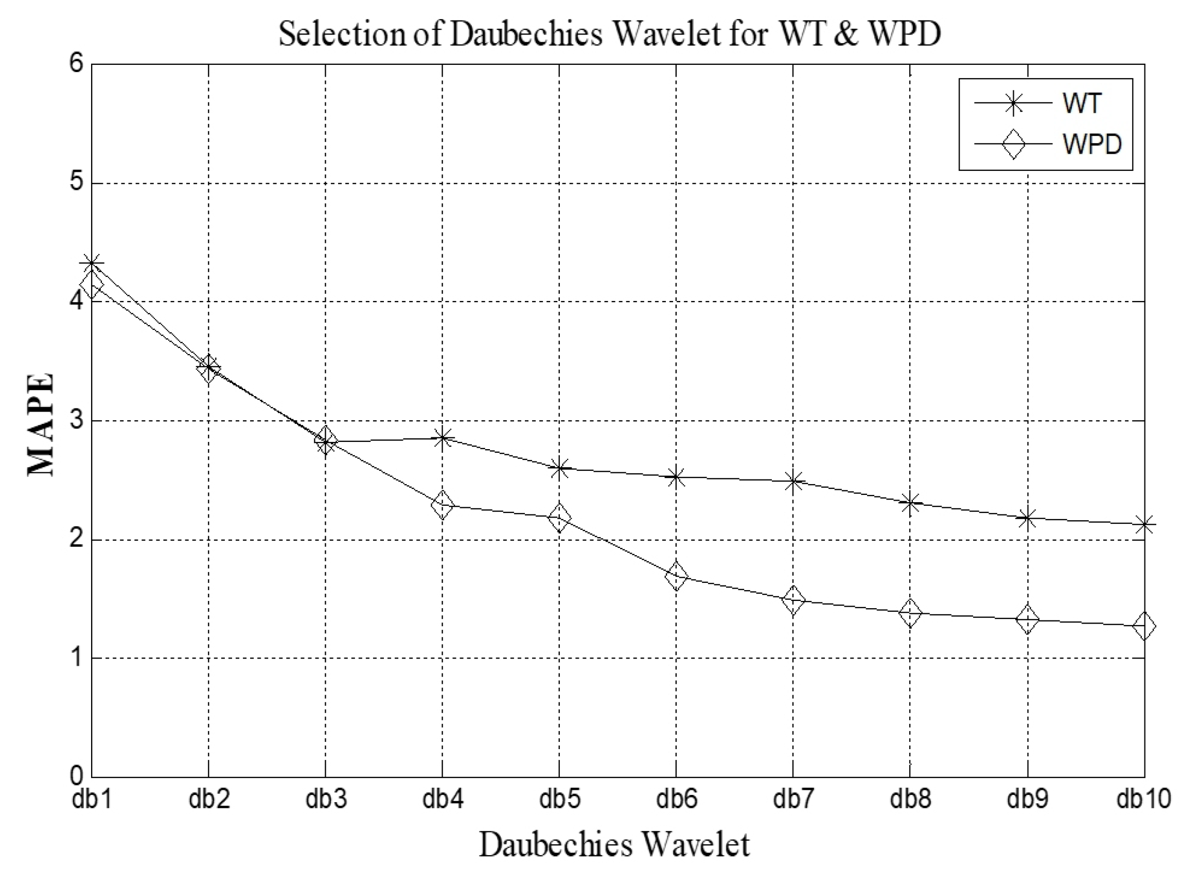
The conventional WT decomposes the signal into low frequency and high-frequency components. However, for better accuracy in the results, the low-frequency component of the signal is further decomposed into the low and high-frequency components using multi-resolution analysis theory. The decomposed series has been further processed through the Group Method of Data Handling (GMDH)-based algorithm for the forecasting of load data series [30]. In 2021, the same decomposition process was carried out for temperature data in which the mother wavelet was chosen on the basis of the energy-entropy ratio; for training and testing data, a different learning algorithm-based NN was proposed [31]. On the other hand, WPD decomposes the load profile between higher and lower frequency components again into lower and higher frequency components with neural networks, and achieved almost 20% more accurate results compared to traditional WT [32]. Advanced WT has been presented in which the entropy cost function is used to select the best wavelet basis for data decomposition, mutual information for feature selection, and neural networks for prediction of electricity load with a one and multi-step-ahead basis [33]. 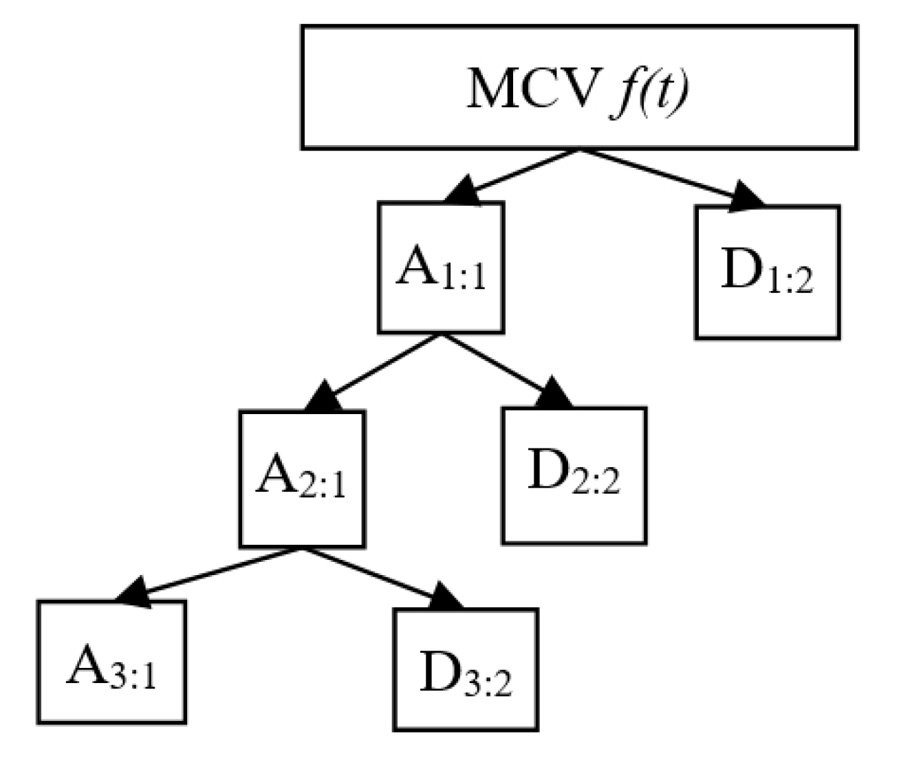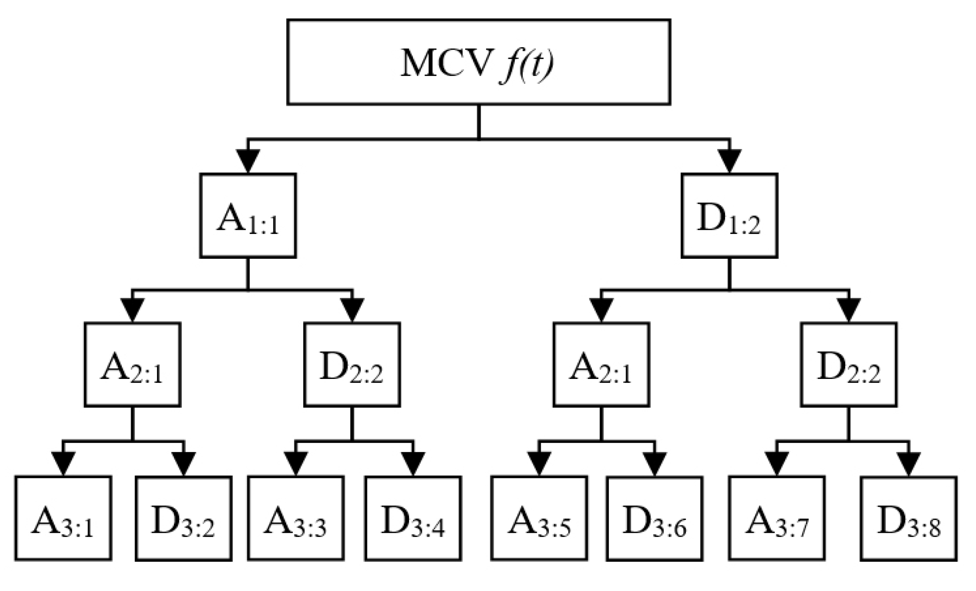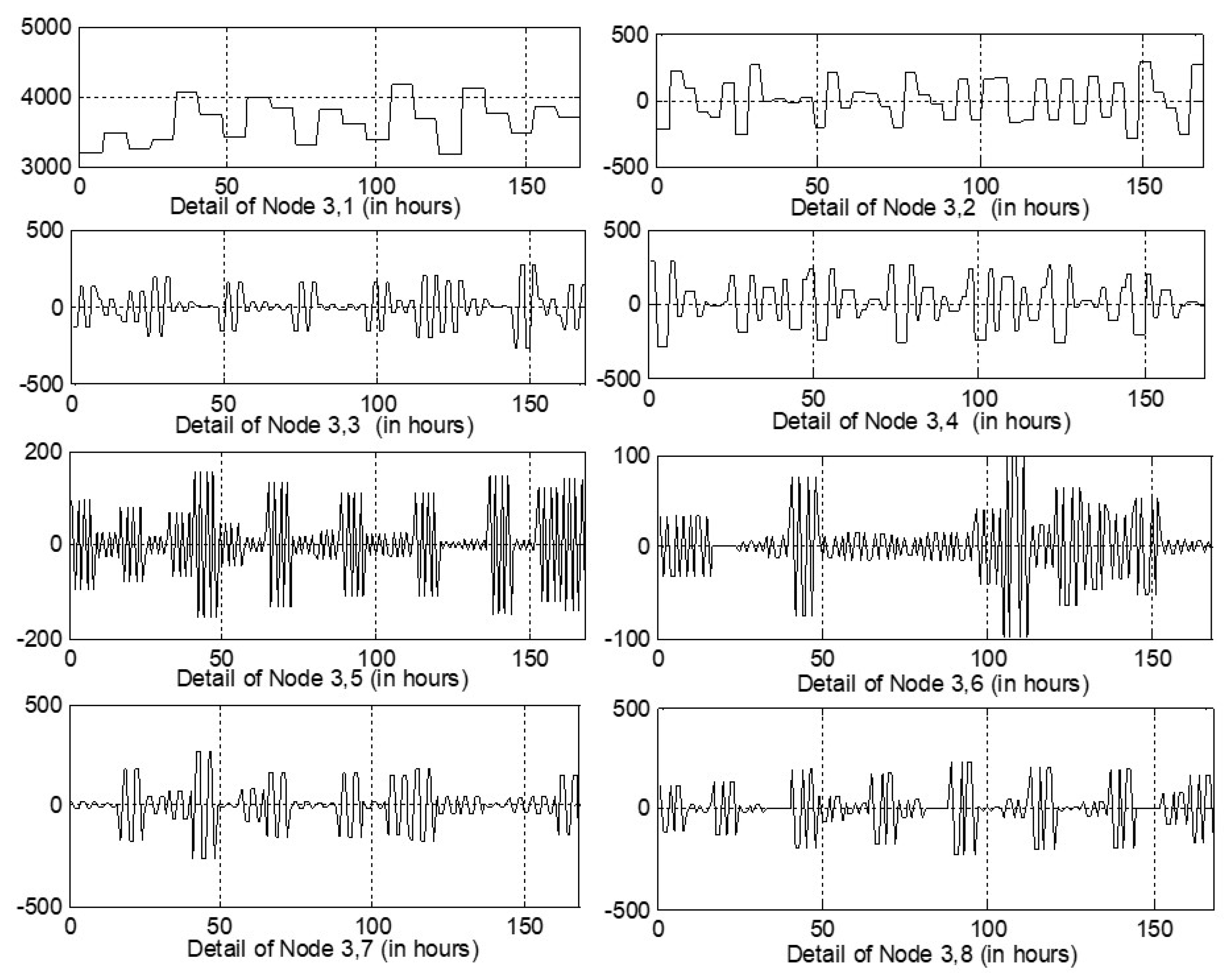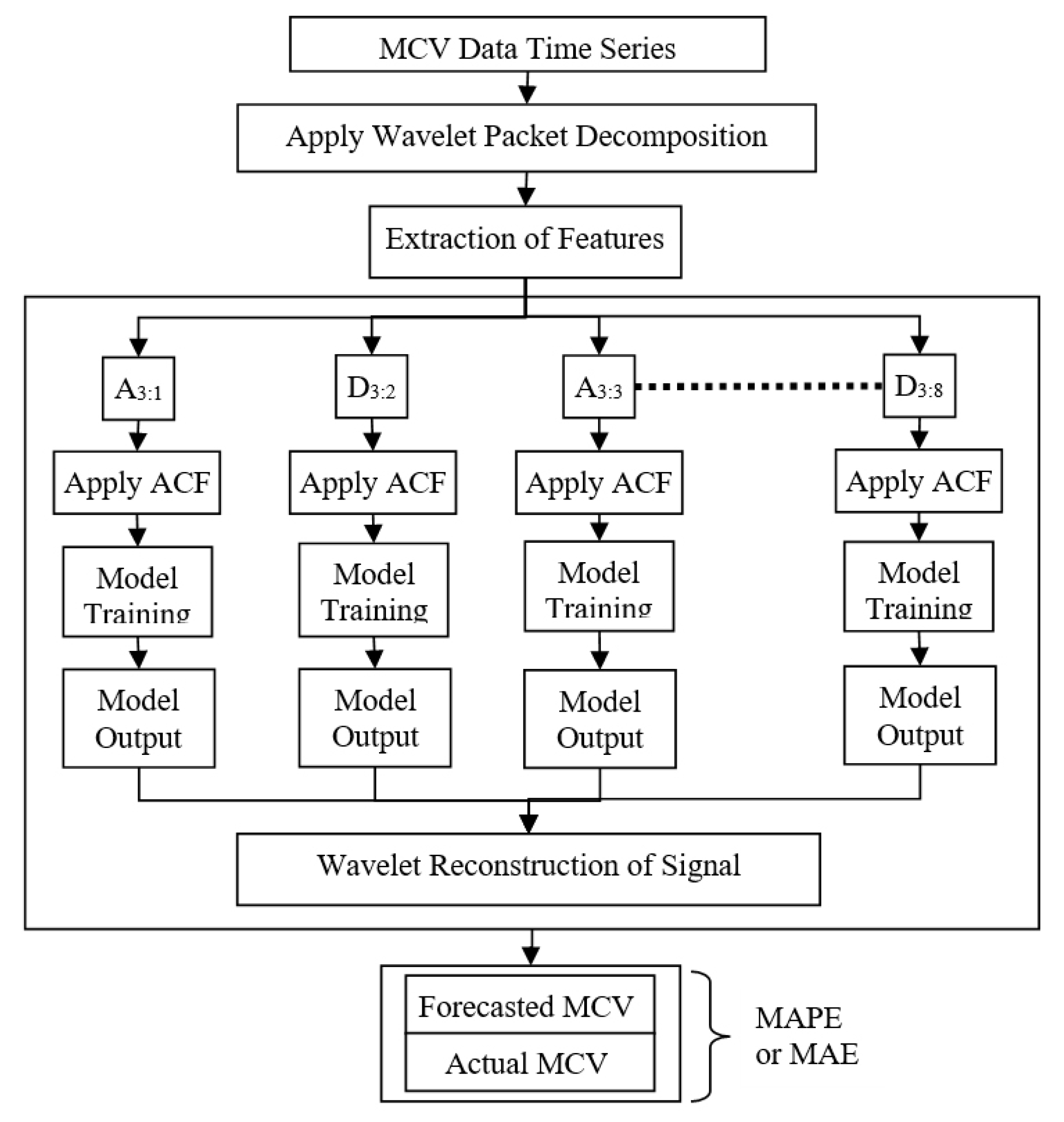In order to deal with the data noise of WPD, decomposed series correlation analysis has been deployed, and data with all the features has been trained through an improved weighted extreme learning machine [34]. In this paper, to extract the maximum features of the input signal, the data was decomposed using the proposed signal processing technique, i.e., WPD. Unlike WT, it decomposes approximate and detailed components at the same time to achieve the maximum resolution to the input data.

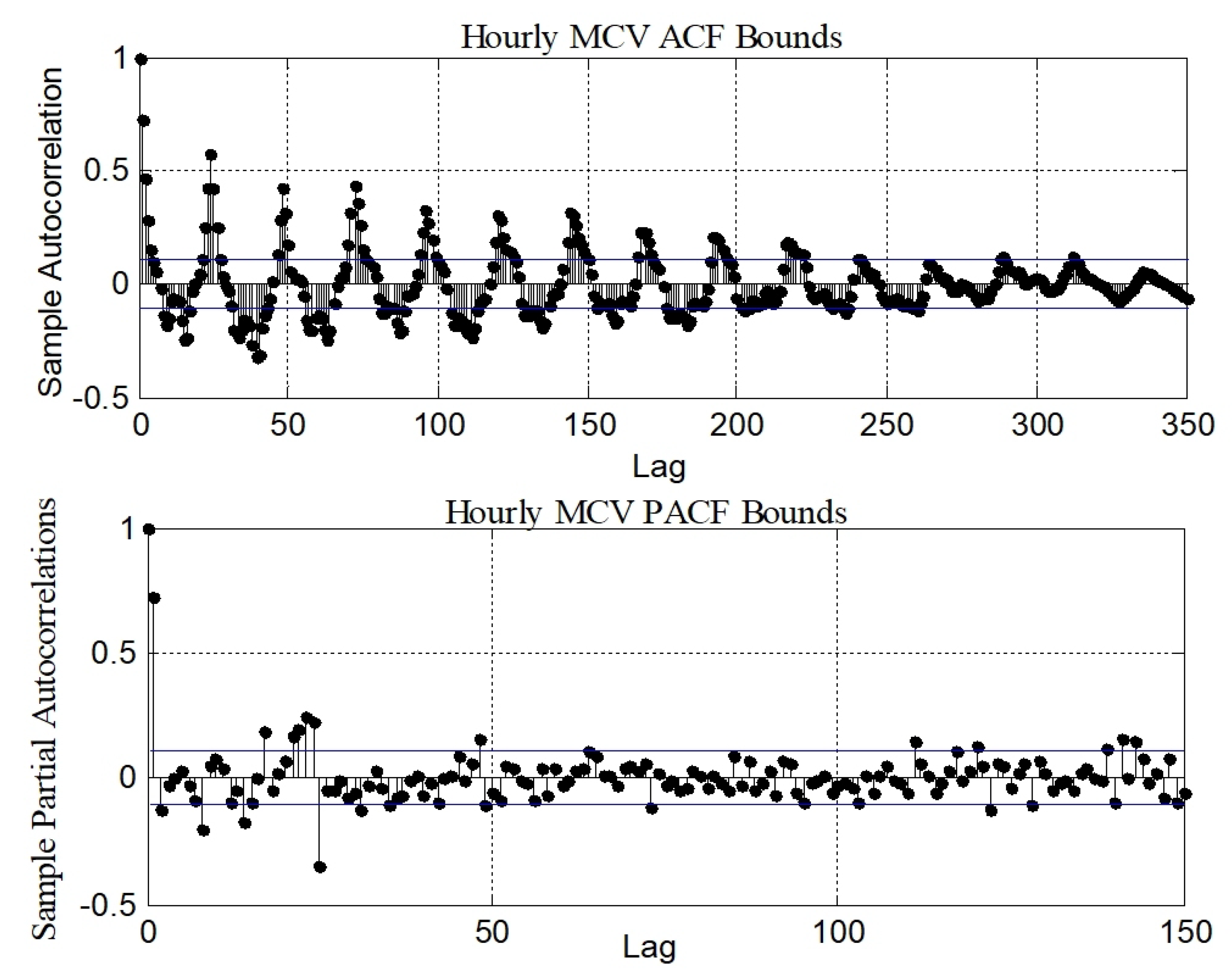
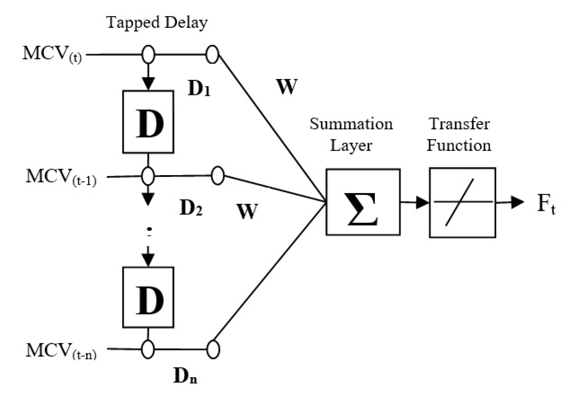
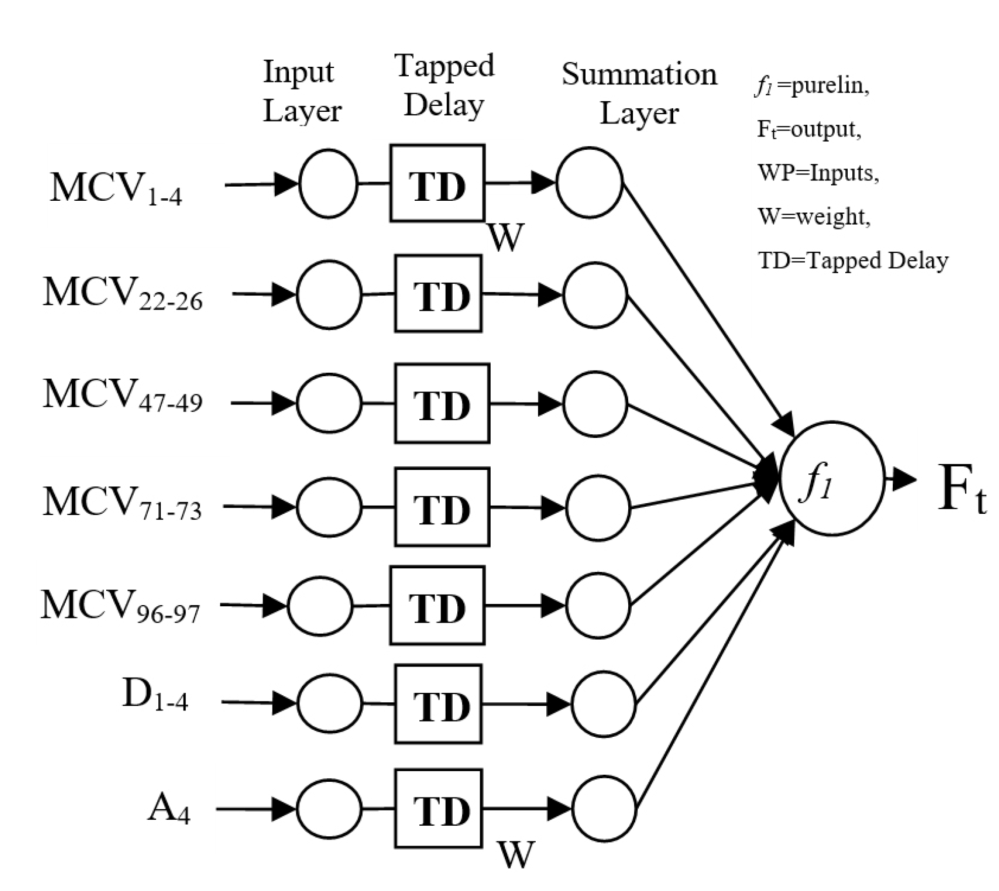
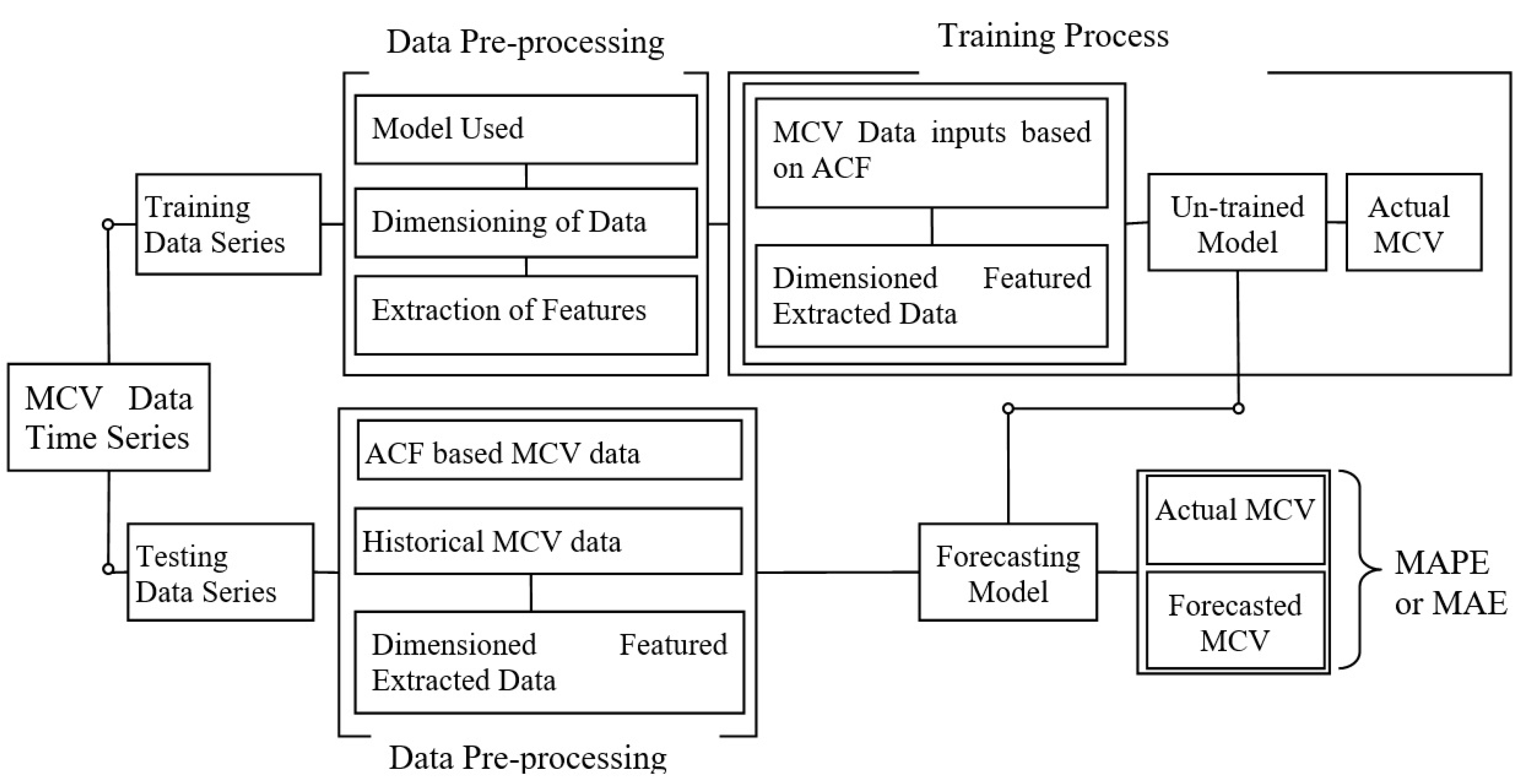
As per the existing literature, it has been observed that the pre-processing of data is still an open issue from the forecasting point of view. Therefore, in this, the authors proposed a time series (statistical)-based forecasting model in which WPD is used as an input data pre-processing tool for MCV forecasting. The results of the proposed model have been compared with stand-alone NN and conventional WT-based models for a single step ahead of point forecasting. The contribution is summarised as follows: First, a practical and transparent approach with the newly demonstrated LNNTD model has been implemented to forecast MCV; the input neurons of this have been selected using ACF. Second, the proposed MCV forecast framework has been implemented to forecast MCV for a period of one year with all seasonal estimation weeks. The concept of a moving window has been adapted with a cyclic test period of one month up to a one year forecast using the one-year training data set. In WPD-based models, two types of input selection criteria have been adopted; first, one combination of WPD-based decomposed series with ACF-based time lags (TL’s) have been used as input vectors (neurons) of the model, and a similar theory has also been used for conventional WT-based models. In later (proposed) models, each WPD-based series has been forecasted individually, and the TL’s for this have been selected on the basis of mutual correlation among all time-lags using ACF. Third, as per the existing literature, for the very first time, TS’s of the forecasts have been measured for the validation of results on a single step-ahead of the forecasted values. The multiple step-ahead forecasting is conducted using an iterative approach up to the sixth step to check whether the forecast is applicable or not. Next, Section 2 describes the strategy of the proposed model, the experimental work is presented in Section 3, the Discussion is in Section 4, and finally the paper is concluded in Section 5.

2. Strategy of Proposed Model

In this section, the authors have tried to take care of all the methodology associated with MCV forecasting, with an aim to improve the accuracy of forecasts. The proposed model utilized the features of WPD as a pre-processing tool for LNNTD. In this model, each preprocessed sub-series was forecasted individually, and the input features were chosen on the basis of mutual correlation among the TL’s using ACF. The performance of the proposed model was compared with standard benchmark stand-alone NN models such as Feed Forward Neural Networks (FFNN), GA-based NN (GANN), and Elman Recurrent Neural Networks (ERNN), along with conventional WT-based NN models. The structural parameters of all compared models are discussed in this section. An extensive study for the selection of wavelet selection has also been carried out on all accuracy indices. The details are described in the next subsections.

2.1. Input Selection

The demand curve of electricity has been associated with various uncertain factors that will be reflected in the MCV curve. These factors affect the training and weight adjustment of neural networks that create difficulties during the input selection of NN models. Therefore, there is a requirement for special treatment for input selection. The selection of input variables is one of the most important parts of NN-based forecasting models. The input vector (neurons) determines the input architecture of the NN model on which the accuracy of the model is highly dependent. In the present work, a correlation-based time series method has been utilized to select the input time lag data, and the proposed model has been effectively implemented on the two year (2015–2016) IEX unconstrained MCV data [35].

In the time series context, it is necessary to know the relationship that exists between the present-time MCV series, along with their past time-lag series. The ACF and partial autocorrelation function (PACF) have been used for input selection. ACF and PACF plots of a sample MCV series are shown in Figure 1. The higher value of ACF defines the correlation between successive lags, which is very strong and drops off very quickly over large time lags. The MCV curve forecast problem aims to find an estimate $MC{V}_{(t+k)}$ of the MCV curve the vector $MC{V}_{(t+n)}$ based on the previous n measurements: $MC{V}_{\left(t\right)}$, $MC{V}_{(t-1)}$, …, $W{P}_{(t-n)}$. The number of time lags are 17 as: $MC{V}_{(t-97)}$, $MC{V}_{(t-96)}$, $MC{V}_{(t-73)}$, $MC{V}_{(t-72)}$, $MC{V}_{(t-71)}$, $MC{V}_{(t-49)}$, $MC{V}_{(t-48)}$, $MC{V}_{(t-47)}$, $MC{V}_{(t-26)}$, $MC{V}_{(t-25})$, $MC{V}_{(t-24)}$, $MC{V}_{(t-23)}$, $MC{V}_{(t-22)}$, $MC{V}_{(t-4)}$, $MC{V}_{(t-3)}$, $MC{V}_{(t-2)}$, $MC{V}_{(t-1)}$.

2.2. Pre-Processing Using Wavelet Transform

In this step, two types of wavelet theories have been adopted for the preprocessing of data, first one is conventional Wavelet Transform (WT) and the second is Wavelet Packet-based Decomposition (WPD).

2.2.1. Conventional Wavelet Transform (WT)

For an MCV forecasting model, it is necessary to pre-process the input data because of uncertainty and nonlinearity. The MCV time-series signal collected from the site might be associated with some corrupted and irrelevant information. This corrupted time series needs to be improved using WT. It is a mathematical signal processing tool used to handle the continuous time-varying signal, and divide the original time series into subseries that forecasts better than the original. Based on the time series signal category, WT is of two types: continuous and discrete wavelet transforms.

For an input MCV signal, MCV(t), the continuous wavelet transform (CWT) is defined on the real axis from (-infinity to infinity) and is given as:

$$W(a,b)=a^{-\frac{1}{2}}{\int }_{-\infty }^{\infty }MCV\left(t\right)·{\psi }^{\ast }\left(\frac{t-b}{a}\right)dt$$

(1)

where: a is the scaling function of the mother wavelet function $W(a,b)$, b is the time-shifting translation variables, ${}^{\ast }$ denotes the complex conjugate, and $\psi \left(t\right)$ denotes the mother wavelet.

CWT is the continuous scaling and time-shifting of the mother wavelet to either the high-scaled sub-frequency component or low-scaled sub-frequency component. The high-scaled (low-pass filter) and low-scaled (high-pass filter) frequency components provide approximate and detailed information about the input MCV signal.

Whereas, in discrete wavelet transforms (DWT), discrete scaling $(a=2i)$ and time-shifting $(b=k^{2i})$ of the mother wavelet function $W(a,b)$ are done. Using DWT, the decomposition and reconstruction of the original MCV signal are followed by (2):

$$W(a,b)=\frac{1}{\sqrt{2^i}}{\int }_{-\infty }^{\infty }MCV\left(t\right)·{\psi }^{\ast }\left(\frac{t-2^{i}k}{2^i}\right)dt$$

(2)

DWT involves both high-pass and low-pass filters corresponding to decomposition and reconstruction of the original MCV data pattern [20,21]. The approximate $(A_1,A_2,\dots ,A_N)$ and detailed coefficient $(D_1,D_2,\dots ,D_N)$ of MCV data signal, $MCV\left(t\right)$, is given below in Figure 2 as per the multi level decomposition (3):

$$MCV\left(t\right)=D_1+D_2+D_3+...+D_N+A_1+A_2+A_3+...+A_N$$

(3)

2.2.2. Wavelet Packet Based Decomposition (WPD)

In WPD, the WT-based decomposed approximated signal components with low frequencies and the detailed signal components with high frequencies have been further decomposed. Therefore, by using WPD-based decomposition, more valuable information can be extracted from the original raw time series of MCV. The original time series of MCV has been decomposed into four sets of approximated and detailed signals: (A3:1, D3:2), (A3:3, D3:4), (A3:5, D3:6), (A3; 7, D3:8) up-to third level of decomposition as shown in Figure 3 and the waveform is shown in Figure 4. The Daubechies (db) wavelet has been shown to be one of the most capable of dealing with MCV data and the analysis for the selection of $db$ has been discussed in Section 2.5. These technique outputs are much more balanced compared to that of WT, and this can easily identify weak and singular component signals. If $\theta \left(t\right)$ is the scaling function, and $\psi \left(t\right)$ is the wavelet function, then both can be related, as [31,34]:

$$\left\{\begin{array}{c}\hfill \theta \left(t\right)=\sqrt{2}\sum _m{l}_{im}\theta (2t-m)\hfill \\ \hfill \psi \left(t\right)=\sqrt{2}\sum _m{h}_{im}\psi (2t-m)\hfill \end{array}\right.$$

(4)

In Equation (4), $l_{im}$ and $h_{im}$ denotes the low- and high-pass frequency coefficients of the signal, respectively. The full wavelet packet $\left\{{\delta }_n\left(t\right)\right\}(n\in Z_{+})$ is on the basis of ${\delta }_o\left(t\right)=\theta \left(t\right)$, which can be derived as:

$$\left\{\begin{array}{c}\hfill {\delta }_{2n}\left(t\right)=\sqrt{2}\sum _m{h}_m{V}_n(2t-m)\hfill \\ \hfill {\delta }_{2n+1}\left(t\right)=\sqrt{2}\sum _m{g}_m{V}_n(2t-m)\hfill \end{array}\right.$$

(5)

In the above Equation (5), $h_m$ and $g_m$ are the wavelet function coefficients, v is the wavelet packet (WP), n denotes the decomposition level in which b is the node position at that level where convolution of the wavelet and scaling filter with WP of the previous level can be used to generate the wavelet packet coefficient at a specific level. This process is repeated until the desired depth of the binary tree is reached.

2.3. Linear Neural Network with Time Delay

The Linear Neural Network (LNN) is a three-layer NN in which the transfer function used is linear rather than hard-limiting. In LNN, there is a delay between the input and summation layer as shown in Figure 5.

The input MCV data pattern is fed to the input layer and passed via the n delays of the Finite Impulse Response (FIR) filter to the summation layer. The output signal that comes out from the summation layer is passed through the linear transfer function to the output layer. It combines the features of the Multi-Layer Perceptron (MLP) structure with a delay layer between the input and summation layers [36,37,38,39]. The output of the network has been evaluated using Equation (6). The network has been trained using the standard Back Propagation algorithm (BP).

$$F_t=purelin(w_p+b)=\sum _{i=1}^R{w}_{1,i}MCV(k-1+1)+b$$

(6)

where $F_t$ is the output response of the network, w is the weight matrix, $MCV(k-1+1)$ is the $(k-1)$ time delay in the MCV signal, b is the bias, and the activation function used is pure linear $\left(purelin\right)$.

The basic structures of both NN and WT-based NN with the proposed model have been given in

Table 1. Structure of all models used.

Model	Learning Algorithms	Input Neurons	Transfer Function	Momentum Constant	Learning Rate
FFNN	LM	17	tansig, purelin	0.06	0.001
ERNN	LM	17	tansig, purelin	0.06	0.001
GANN	GA	17	tansig, purelin	0.06	0.001
LNNTD	BP	17	purelin	0.06	0.001
WT+LNNTD	BP	$17+5$	purelin	0.06	0.001
WPD+LNNTD	BP	$17+8$	purelin	0.06	0.001
Proposed	BP	-	purelin	0.06	0.001

. The NN model input architecture consists of time-domain variables only; whereas, conventional WT-based models are fed the time domain as well as the wavelet domain variables (Figure 6). The structure of the proposed WPD-based model is also the same as that of other models, except for that of input neurons, which have been detailed in

Table 2. Time lags (features) for wavelet component forecasts.

Wavelet Component	Selected Time Lags for Forecasting Target Series (T)
D30	TL_10, TL_9, TL_8, TL_7, T_6, TL_5, TL_4, TL_3, TL_2, TL_1
D31	TL_19, TL_18, TL_17, T_16, TL_15, TL_14, TL_13, TL_12, TL_11,
	TL_10, TL_9, TL_8, TL_7, T_6, TL_5, TL_4, TL_3, TL_2, TL_1
D32	TL_25, TL_12, TL_11, TL_10, TL_9, TL_8, TL_7, T_6, TL_5, TL_4,
	TL_3, TL_2, TL_1
D33	TL_28, TL_25, TL_21, TL_10, TL_9, TL_8, TL_7, T_6, TL_5, TL_4,
	TL_3, TL_2, TL_1
D34	TL_13, TL_12, TL_11, TL_10, TL_9, TL_8, TL_7, T_6, TL_5, TL_4,
	TL_3, TL_2, TL_1
D35	TL_7, T_6, TL_5, TL_4, TL_3, TL_2, TL_1
D36	TL_8, TL_7, T_6, TL_5, TL_4, TL_3, TL_2, TL_1
D37	TL_9, TL_8, TL_7, T_6, TL_5, TL_4, TL_3, TL_2, TL_1

. The concept of a moving window has been adopted for training and testing of the models, as detailed in Figure 7. To get wavelet sub-series, $db10$ has been used for the multi-scale analysis of MCV.

The forecasting steps are similar for all models, except in cases discussed below:

• Step 1: From raw MCV data, an input time series vector has been formed, on the basis of ACF 17, time-lag data was chosen as the input variable for standalone NN models.
• Step 2: edcomposition of the original MCV time series into approximated (A1–A6) and detailed (D1–D6) subseries using $db10$.
• Step 3: The fourth level approximated and detailed MCV subseries with a 17 MCV time lag has been selected as an input variable for conventional WT-based models. The structure of the LNNTD model is shown in Figure 6 and the schematic flow diagram for the conventional WT-based MCV forecasting model is shown in Figure 8.
• Step 4: For the WPD-based model, a third-level decomposition is used [35,36,37,38,39] in which eight different high- and low-frequency component-based series are obtained. Two types of input selection criteria are adopted first, eight WPD-based decomposed series are used with 17 ACF-based time-lag series similar to that of the conventional WT-based model. In the second (proposed model), each WPD-based series has been forecasted individually, the schematic flow diagram is shown in Figure 9 and the TL’s are selected on the basis of ACF which are presented in Table 2.
• Step 5: For the forecasting, one-year MCV data was trained and tested for the next month, a similar process is continuously repeated up to the next 12 months, with a one-month moving window as shown in Figure 6. The epochs and performance goals have been chosen to be equal to 10,000 and 0.001, respectively.

2.4. Accuracy Metrics

For the accuracy of estimated MCV results, the trained NN forecast output has been compared with the actual indicated MCV values. The comparison has been made with two measures, Mean Absolute Percentage Error (MAPE) and Mean Absolute Error (MAE). The MAPE can be defined as follows:

$$MAPE=\frac{1}{n}\sum _{n=1}^t\left|\frac{(MC{V}_t-F_t)}{MC{V}_t}\right|$$

(7)

The MAE is given by:

$$MAPE=\frac{1}{n}\sum _{t=1}^n\left|(MC{V}_t-F_t)\right|$$

(8)

where $MC{V}_t$ is the actual indicated MCV value, $F_t$ is the estimated MCV value for the tth hour and n is the number of hours considered for forecasting.

2.5. Effect of Pre-Processing on the Performance of the Model

2.5.1. Effect of Conventional WT

Consequently, the application of WT makes the input MCV data patterns more suitable and efficient for accurate forecasting by improving the hidden characteristics of the original MCV data signal. The NN models train themselves in a better way with input sub-frequency data components compared to actual MCV data, which results in better forecasts. For proper selection of decomposition levels, a complete experimental analysis has been done on the basis of their error rate. Based on the ascending order of WT decomposition, the results are drawn in

Table 3. WT analysis for the selection of decomposition.

Decomposition Level	Decomposed Signals	WT	Decomposed Signals	WPD
	db10	MAPE	db10	MAPE
Level 1	A1, D1	3.22	A1:1, D1:2	3.115
Level 2	A2, D1, D2	2.49	A2:1, D2:2, A2:3, D2:4	1.882
Level 3	A3, D1, D2,	2.22	A3:1, D3:2, A3:3, D3:4,	1.258
	D3		A3:5, D3:6, A3:7, D3:8
Level 4	A4, D1, D2,	2.12	A4:1, D4:2, A4:3, D4:4, A4:5,	1.314
	D3, D4		D4:6, A4:7, D4:8, A4:9, D4:10,
			A4:11, D4:12, A4:13, D4:14,
			A4:16, D4:16
Level 5	A5, D1, D2,	2.13	A5:1, D5:2, A5:3, D5:4, A5:5,	6.43
	D3, D4, D5		D5:6, A5:7, D5:8, A5:9, D5:10,
			A5:11, D5:12, A5:13, D5:14, A5:16,
			D5:16, A5:17, D5:18, A5:19, D5:20,
			A5:21, D5:22, A5:23, D5:24, A5:25,
			D5:26, A5:27, D5:28, A5:29, D5:30,
			A5:31, D5:32
Level 6	A6, D1, D2,	2.17	-	-
	D3, D4, D5, D6

and a similar procedure has also been adopted for the selection of Daubechies wavelet as shown in Figure 10. Thus, on the basis of experimental analysis, it is found that the fourth level decompositions using $db10$ provides the best-suited forecasts.

2.5.2. Effect of WPD

On the basis of the existing literature, the third level decomposition using WPD is found to be more suitable [30,31,32,33]. However, for proper selection of decomposition level, a complete experiment has also been conducted to verify the results on the basis of their error rate. Based on the ascending order of WPD decomposition up to the fifth level, the results are shown in Table 3 and a similar procedure has also been adopted for the selection of Daubechies wavelet as shown in Figure 10. From fourth level WPD results it is observed that the error is almost close to the third level but in the fifth level of decomposition, the error is increased suddenly because, in this level, the input variables are almost double to that of the fourth level input variables. Similarly, in the sixth level decomposition, the numbers of input variables are almost double that of the fifth level, they are very difficult to handle and the error rate will also abruptly rise. Thus, on the basis of experimental analyses, it is observed that third-level decomposition using $db10$ provides the best-suited forecasts.

3. Simulation Results

The hourly IEX unconstrained MCV data has been utilized for the evaluation of the performance measurement of presented load forecasting models. The data includes the historical load for a two year period from 2015 and 2016. The authors have not cut out any part of the time-series such as anomalous days, special events, or data that might be flawed. The performance of the stand-alone NN model has been compared with WT-based NN models along with the proposed model. The forecasting performance of all models has been carried out on the basis of accuracy and $R^2$ analysis using MATLAB version R2020b.

3.1. Accuracy Analysis

The performance on the basis of accuracy has been carried out on a monthly and seasonal week basis using MAPE and MAE accuracy indices. The MAPE test results for the year 2016 have been presented in

Table 4. Monthly MCV forecasting accuracy (MAPE 2016).

2016	FFNN	ERNN	GANN	LNNTD	WT+LNNTD	WPD+LNNTD	Proposed
January	2.794	3.686	2.783	2.763	1.641	1.047	0.164
February	2.431	3.197	2.474	2.410	1.563	1.005	0.175
March	3.613	3.969	3.597	3.569	1.848	1.214	0.220
April	3.769	4.069	3.582	3.438	1.624	1.132	0.205
May	3.646	4.555	3.559	3.572	1.788	1.152	0.198
June	2.853	3.383	2.906	2.862	1.528	1.019	0.174
July	2.961	3.047	2.856	2.789	1.331	0.854	0.170
August	3.299	3.571	3.206	3.143	1.635	1.003	0.198
September	3.843	4.634	3.919	3.782	1.658	1.034	0.192
October	4.381	5.014	3.962	3.953	1.793	1.120	0.204
November	4.207	5.469	4.352	4.140	2.410	1.741	0.285
December	3.501	4.392	3.561	3.391	2.219	1.622	0.226
A.V.	3.441	4.082	3.396	3.318	1.753	1.162	0.201

on a monthly average basis. The average MAPE achieved by the ERNN Model is 4.082% (January 2016 to December 2016) which is higher than other NN models; whereas, the value of MAPE for the same period by FFNN, GANN, and LNNTD is 3.441%, 3.396%, and 3.317%, respectively. The monthly average performance on the MAE scale (January 2016 to December 2016) achieved by FFNN, ERNN, GANN, and LNNTD is 161.540 MWh, 190.760 MWh, 159.692 MWh, and 154.954 MWh, respectively, as given in

Table 5. Monthly MCV forecasting accuracy (MAE 2016).

2016	FFNN	ERNN	GANN	LNNTD	WT+LNNTD	WPD+LNNTD	Proposed
January	115.253	151.121	115.221	113.850	67.0143	43.039	6.758
February	103.007	138.273	105.280	102.680	65.7499	42.895	7.398
March	161.492	176.189	161.020	158.840	82.0146	53.843	9.805
April	198.377	214.583	188.657	178.610	83.9282	58.263	10.523
May	149.702	185.845	146.430	146.830	74.4242	47.911	8.0387
June	130.586	153.594	132.857	130.780	68.9155	45.504	7.704
July	146.409	150.990	141.618	137.820	65.9655	41.784	8.249
August	160.145	173.035	156.889	152.300	78.7189	47.937	9.366
September	195.639	235.798	199.298	191.290	84.2253	52.282	9.811
October	219.531	253.934	199.514	197.180	89.0009	54.529	9.973
November	205.628	263.373	214.261	201.730	114.344	81.572	13.454
December	152.716	192.387	155.27	147.560	93.9196	67.216	7.596
A.V.	161.540	190.760	159.693	154.950	80.6851	53.065	9.056

. The performances in terms of MAPE for all stand-alone NN models are almost similar; but, the performance of LNNTD has been found to be better as compared to other stand-alone NN models. Due to this, LNNTD has been used exclusively with pre-processing techniques adopted for the present work. From

Table 6. Indian seasonal time period.

Season	Period	Testing Period
Winter	December–March	week 1
Summer	April–May	week 1
Rainy	June–September	week 1
Dry	October–November	week 1

, the average MAPE performance (January 2016 to December 2016) of WT+LNNTD, WPD+LNNTD and proposed model is 1.753%, 1.162%, and 0.201%, respectively. From

Table 7. Seasonal MAPE MCV estimation accuracy.

Models	Week 1	Week 2	Week 3	Week 4	A.V.
FFNN	2.5142	3.6082	3.415	4.096	3.408
ERNN	3.0571	3.9597	3.966	5.407	4.097
GANN	2.5091	3.7614	3.39	4.127	3.447
LNNTD	2.5345	3.7416	3.393	3.964	3.408
WT+LNNTD	1.5189	1.5274	1.636	1.657	1.585
WPD+LNNTD	1.8174	0.9913	1.0189	1.1304	1.2395
Proposed	0.3008	0.1886	0.1973	0.2134	0.225

, the average MAEs reported by the WT+LNNTD, WPD+LNNTD, and proposed model are 80.6851 MWh, 53.065 MWh, and 9.056 MWh respectively.

It is observed that the performance of all stand-alone NN models is almost the same; but, when WT is deployed for input pre-processing; then, there is improvement in results to a large extent. Therefore, the improved results confirm the utility of WT for input pre-processing. These are the observations obtained from an accuracy point of view:

• The performance in terms of accuracy of LNNTD is the best among all NN models.
• WT-based NN model accuracy is higher compared to the NN models.
• The accuracy level of the proposed model is found to be better amongst all others.
• In spite of that, FFNN is one of the toughest benchmarks to beat.

In order to check the quality of the forecasts, four seasonal weeks presented in Table 6 [40] has also been taken into consideration. The forecasted results in terms of MAPE and MAE have been given in Table 7 and

Table 8. Seasonal MAE MCV estimation accuracy.

Models	Week 1	Week 2	Week 3	Week 4	A.V.
FFNN	100.747	177.882	161.195	241.018	170.211
ERNN	121.359	195.231	185.157	323.919	206.417
GANN	100.576	185.298	159.586	244.208	172.417
LNNTD	101.137	184.009	159.882	231.445	169.118
WT+LNNTD	58.957	75.0393	74.9522	96.5705	76.3797
WPD+LNNTD	70.9611	50.0129	48.34038	63.3021	58.1541
Proposed	12.0576	9.45813	9.246981	11.9904	10.6883

, respectively. The proposed model also performed better than others with an average MAPE of 0.225% and MAE of 10.688 MWh and the percentage of improvement is discussed in the Discussion section. To check the viability of the forecasting tools used, the seasonal week’s actual and forecasted MCV with the error curve has been presented in the given Figure 11, Figure 12, Figure 13 and Figure 14. These curves have been considered because all seasons have different demand curve variations.

3.2. Coefficient of Regression $R^2$ Analysis

The $R^2$ has been utilized to articulate the slope of the forecasted MCV against the actual value of MCV as described in

Table 9. Overall forecasting coefficient of regression $R^2$.

Models	FFNN	ERNN	GANN	LNNTD	WT+LNNTD	WPD+LNNTD	Proposed
January	0.959	0.97	0.968	0.923	0.977	0.990	0.9997
February	0.917	0.855	0.912	0.916	0.970	0.987	0.9996
March	0.873	0.851	0.873	0.875	0.972	0.987	0.9995
April	0.859	0.833	0.866	0.868	0.973	0.986	0.9996
May	0.873	0.811	0.876	0.876	0.971	0.988	0.9996
June	0.916	0.891	0.912	0.913	0.980	0.991	0.9997
July	0.908	0.898	0.912	0.915	0.982	0.993	0.9997
August	0.925	0.913	0.926	0.928	0.983	0.994	0.9997
September	0.851	0.803	0.843	0.853	0.975	0.990	0.9996
October	0.654	0.875	0.916	0.919	0.984	0.994	0.9998
November	0.912	0.865	0.901	0.913	0.977	0.988	0.9996
December	0.933	0.904	0.927	0.937	0.979	0.989	0.9997
A.V.	0.882	0.872	0.903	0.903	0.977	0.990	0.9996

. The average value of $R^2$ determined for the year 2016 by FFNN is 0.882, which is almost similar to that of all NN models. Furthermore, LNNTD also outperformed in our study, with a value of 0.9034. However, the value of $R^2$, determined by the WT-based model is better than NN models, which are close to unity (by proposed 0.9996). When forecasting accuracy is poor, then $R^2$ moves away from unity; when accuracy is better then it moves close to unity.

4. Disscusion

In this section, the proposed model performance has been validated on the basis of the calculation of forecast tracking signals, and the universality of the model has been carried out using multiple-step ahead forecasts up to six steps. Further, in order to investigate the forecasting performance, the percentage of improvement in accuracy has also been taken into consideration.

4.1. Validation of the Model Using Tracking Signals (TS’s)

In 1962, Brown has introduced TS’s with an objective to provide automatic quality control for the forecasting system [41]. The purpose is to find whether the forecast is absolute or misbehaving on the data set. Generally, it is applied to a system that covers thousands of data points and where the data set is highly influenced by unsuspected seasonal variations. From the forecasting point of view, it is necessary to predict such situations within a quick succession of time so that a more appropriate and accurate model may be introduced. It is defined as the sum of the forecasting errors divided by the mean absolute deviation [42,43]. TS’s are very helpful to find out whether our forecasting model is balanced or moving in one direction, i.e., over-forecasted or under-forecasted. For balanced forecasts, its values should be close to zero and move in both directions, positive as well as negative. The positive value of TS suggests that the model output is less than the actual value (under forecast); whereas, a negative value of TS conveys that model output is higher than the actual value (over forecast). When a forecast is consistent in one direction, either positive or negative, then it is referred to as biased forecasting. Here, the meaning of biasness is the continuous deviation of forecasts from the mean in one direction. So, it is a very helpful tool for us in improving or adapting the forecasting model in real-time situations [43,44].

$$TrackingError=\frac{SumofError}{MeanAbsoluteDeviation\left(MAD\right)ofError}$$

(9)

$$SumofError=PreciousSumofErrors+LatestError$$

(10)

$$MAD=\frac{SumofAbsoluteError}{NumbersofObservations}$$

(11)

Table 10. Overall forecasting tracking signal (TS).

Models	FFNN	ERNN	GANN	LNNTD	WT+LNNTD	WPD+LNNTD	Proposed
January	−34.78	68.77	−23.3	7.92	−4.12	−15.11	0.57
February	−18.06	65.92	−4.36	44.24	8.11	−4.27	2.46
March	88.32	60.51	99.98	80.86	99.48	−2.01	2.62
April	257.81	278.8	261.26	127.48	41.55	−28.49	4.84
May	−97.35	−83.9	−68.25	−31.01	39.91	−5.29	−1.00
June	50.512	50.8	75.72	43.48	12.52	−0.37	2.50
July	104.03	57.02	87.04	83.65	37.69	−16.34	3.05
August	−4.562	24.56	65.50	70.48	83.89	−4.40	4.11
September	49.949	−32.7	43.63	72.82	133.80	−15.19	6.83
October	−27	196.3	86.81	13.39	13.36	−20.07	−0.24
November	43.307	−30.9	55.79	35.45	3.65	−5.75	0.90
December	−120.5	−3.39	−116.8	−38.15	2.16	4.05	−4.92

contains the value of overall TS’s for stand-alone, pre-processing-based and proposed models. As far as the under and over forecasting is concerned that all models have both positive as well as negative values of TS except for one or two models. In the case of stand-alone models, the range of tracking signals is very far away from zero, but has both positive as well as negative values of tracking signals. Their range is high because their performance in terms of accuracy was also poor. On the other hand, the preprocessing-based models have a lower range of TS’s and they are found to be the best with the maximum value of the tracking signal 6.839 for the month of September and a lower value of tracking signal is −4.9257 for the month of December. Hence, the proposed model has more accurate and balanced forecasts among the others because of the positive and negative values.

In spite of the accurate forecast, the TS’s may be out of range because of over- and under-forecasting, and it can be seen from the comparison of the tracking signal and error signals. As per the MAPE and MAE table, the accuracy of WPD is higher with average MAPE and MAE of 1.162% and 53.065 MWh, respectively. On the other hand, the majority of tracking signals for WPD-based model lies in the negative direction with the value of −28.4919 and the maximum value of the tracking signal in positive is 4.056883 for the month of December. Whereas, the majority of tracking signals for WT+LNNTD-based model lies in positive with a maximum value of 133.80 and the only value of tracking signal lies in negative is for January with −4.126882. Therefore, the forecasts are not balanced. Hence, the value of the TS’s depends not only on the accuracy, but also on under- and over-forecasted values of the model used.

4.2. Multiple Steps-Ahead Forecasting

The performance of the proposed model has also been evaluated for more than one, to check the universality of forecasts. In this case, the forecasting is done for more than one hour or day in advance. For multiple-step-ahead forecasting, a single model was trained multiple times depending on the number of steps, and only the target set was changed, corresponding to the number of steps. The target matrix was increased with respect to each step in advance, as given below in Equations (12) and (13). If the large forecasting horizon is considered, the error that occurs at the first step will be multiplied with each step; therefore, the accuracy of the model will be lower. The results in the given

Table 11. Multiple steps-ahead forecasting.

Models	Metrics	Step 1	Step 2	Step 3	Step 4	Step 5	Step 6
FFNN	MAPE	2.78	3.99	4.80	6.57	8.68	9.89
FFNN	MAE	114.97	165.64	196.21	270.32	354.35	404.99
ERNN	MAPE	3.28	4.281	5.18	7.02	8.85	10.03
ERNN	MAE	134.52	174.57	211.98	291.23	365.59	414.12
GANN	MAPE	2.85	3.83	4.66	6.62	8.67	10.01
GANN	MAE	117.44	157.51	191.88	272.66	353.79	410.55
LNNTD	MAPE	2.76	3.87	4.62	6.35	8.31	9.57
LNNTD	MAE	113.84	159.05	189.68	260.87	341.33	393.74
WTLNNTD	MAPE	1.62	2.69	3.31	4.77	5.50	6.10
WTLNNTD	MAE	66.19	110.32	137.06	196.34	226.94	249.91
WPD+LNNTD	MAPE	1.04	2.32	3.04	4.27	5.17	5.81
WPD+LNNTD	MAE	43.03	95.11	125.95	175.76	213.25	238.35
Proposed	MAPE	0.19	0.37	0.59	1.07	1.34	1.57
Proposed	MAE	7.07	15.22	24.23	44.02	54.76	63.29

showed the superiority of the proposed model for six-step-ahead forecasting. The proposed model has achieved a MAPE of 1.57% and a MAE of 63.29 MWh for the sixth step-ahead forecasting in contrast to other models.

$$FirstStep=\left[\begin{array}{cccc}MC{V}_{11}& MC{V}_{12}& ---& MC{V}_{1n}\\ MC{V}_{21}& MC{V}_{22}& ---& MC{V}_{2n}\\ & & & \\ MC{V}_{n1}& MC{V}_{n2}& ---& MC{V}_{nn}\end{array}\right]\left[\begin{array}{c}{T}_1\\ T_2\\ \\ T_n\end{array}\right]$$

(12)

$$n\mathrm{th}Step=\left[\begin{array}{cccc}MC{V}_{11}& MC{V}_{12}& ---& MC{V}_{1n}\\ MC{V}_{21}& MC{V}_{22}& ---& MC{V}_{2n}\\ & & & \\ MC{V}_{n1}& MC{V}_{n2}& ---& MC{V}_{nn}\end{array}\right]\left[\begin{array}{c}{T}_k\\ T_{k+1}\\ \\ T_{K+n}\end{array}\right]$$

(13)

4.3. Percentage of Improvement in Accuracy

The percentage of improvement in accuracy is also one of the criteria for investigating the forecasting performance of a model more comprehensively. Both seasonally, as well as yearly, average MAPE and MAE, have been considered for comparison points of view.

Table 12. Percentage of improvement in MAPE (${\gamma }_{MAPE}$) by the proposed model.

Seasons	FFNN	ERNN	GANN	LNNTD	WT+LNNTD	WPD+LNNTD
Yearly	94.15	95.07	94.08	93.94	88.53	82.70
Winter	88.03	90.16	88.01	88.13	80.19	83.44
Summer	94.77	95.23	94.98	94.95	87.65	80.97
Rainy	94.22	95.02	94.17	94.18	87.94	80.63
Dry	94.79	96.05	94.82	94.61	87.12	81.12

shows the percentage in the improvement of MAPE by the proposed model, with respect to each model utilized in this work, is calculated by the following:

$${\gamma }_{MAPE}=\frac{Y_p-Y_r}{Y_r}\times 100$$

(14)

$${\gamma }_{MAE}=\frac{Y_p-Y_r}{Y_r}\times 100$$

(15)

In the above Equations (14) and (15), $Y_p$ represents the forecasted results of the proposed model and on the other hand, $Y_r$ represents the forecasted results of other models used in this work for performance comparison. Table 12 and

Table 13. Percentage of improvement in MAE (${\gamma }_{MAE}$) by the proposed model.

Seasons	FFNN	ERNN	GANN	LNNTD	WT+LNNTD	WPD+LNNTD
Yearly	94.39	95.25	94.32	94.15	88.77	82.93
Winter	88.03	90.06	88.01	88.07	79.54	83.00
Summer	94.68	95.15	94.89	94.85	87.39	81.08
Rainy	94.26	95.00	94.20	94.21	87.66	80.87
Dry	95.02	96.29	95.09	94.81	87.58	81.05

confirm the superiority of the proposed model which improves the error percentage to a significant level, and for the interpretation of results both MAPE and MAE have been considered. Compared to other models (both stand-alone NN and WT-based models), the yearly average forecast, is increased in the range from 82.702 to 94.15882.9 in the proposed model MAPE, and MAE is increased in the range from 82.93414 to 94.39396. Similarly, the percentage of improvement of results on the basis of MAPE and MAE has been increased for the case of seasonal forecast in the range from 80.635 to 96.053 and 80.87127 to 96.29833, respectively.

5. Conclusions

For appropriate electricity management, taking part in the electricity market bidding and for proper implementation of policies, an accurate load estimation tool is quite important. Electrical engineers and policymakers are working to satisfy various frequency load demand cycles. However, in developing countries, it is very difficult to match the demand and load curve leading to difficulty in designing accurate forecasting tools. Therefore, it has been worth analyzing yearly MCV forecasting performance, in terms of accuracy and the $R^2$ value. It has been observed that the average forecasted MAPE and MAE results obtained by the proposed model are 0.201% and 9.056 MWh, respectively, which is far better than the other respective models. The comprehensive experimental analysis on the tracking signals of the forecast, multiple steps-ahead forecasting, and the percentage of improvement of accuracy indicate the superiority of the proposed model. The observed values of tracking signals, forecast at multiple steps, and the percentage of improvement of accuracy proved the superiority of the proposed model. Furthermore, the results in terms of accuracy can be improved by the more efficient handling of input data through pre-processing and post-processing soft computing-based tools.

References

1. Hippert, H.S.; Pedreira, C.E.; Souza, R.C. Neural networks for short-term load forecasting: A review and evaluation. IEEE Trans. Power Syst. 2001, 16, 44–55. [Google Scholar] [CrossRef]
2. Felice, M.D.; Yao, X. Short-term load forecasting with neural network ensembles: A comparative study. IEEE Comput. Intell. Mag. 2011, 6, 47–56. [Google Scholar] [CrossRef]
3. Vaghefi, A.; Jafari, M.A.; Bisse, E.; Lu, Y.; Brouwer, J. Modeling and forecasting of cooling and electricity load demand. Appl. Energy 2014, 136, 186–196. [Google Scholar] [CrossRef] [Green Version]
4. Saroha, S.; Verma, R. Cross-border Power Trading Model for South Asian Regional Power Pool. Electr. Power Energy Syst. 2013, 44, 146–152. [Google Scholar] [CrossRef]
5. Hahn, H.; Meyer-Nieberg, S.; Pickl, S. Electric load forecasting methods: Tools for decision making. Eur. J. Oper. Res. 2009, 199, 902–907. [Google Scholar] [CrossRef]
6. Aggarwal, S.K.; Saini, L.M.; Kumar, A. Electricity price forecasting in deregulated markets: A review and evaluation. Int. J. Electr. Power Energy Syst. 2009, 31, 13–22. [Google Scholar] [CrossRef]
7. Saroha, S.; Aggarwal, S.K. A Review and Evaluation of Current Wind Power Prediction Technologies. WSEAS Trans. Power Syst. 2015, 10, 1–12. Available online: http://www.wseas.org/multimedia/journals/power/2015/a025716-278.pdf (accessed on 10 May 2021).
8. Babu, K.V.N.; Edla, D.R. New Algebraic Activation Function for Multi-Layered Feed Forward Neural Networks. IETE J. Res. 2017, 63, 71–79. [Google Scholar] [CrossRef]
9. Khotanzad, A.; Zhou, E.; Elragal, H. A neuro-fuzzy approach to short-term load forecasting in a price-sensitive environment. IEEE Trans. Power Syst. 2002, 17, 1273–1282. [Google Scholar] [CrossRef]
10. Ling, S.H.; Leung, F.H.F.; Lam, H.K.; Tam, P.K.S. Short-Term Electric Load Forecasting Based on a Neural Fuzzy Network. IEEE Trans. Ind. Electron. 2003, 50, 1305–1316. [Google Scholar] [CrossRef]
11. Kebriaei, H.; Araabi, B.N.; Rahimi-Kian, A. Short-term load forecasting with a new nonsymmetric penalty function. IEEE Trans. Power Syst. 2011, 26, 1817–1825. [Google Scholar] [CrossRef]
12. Bashir, Z.A.; El-Hawary, M.E. Applying wavelets to short-term load forecasting using PSO-based neural networks. IEEE Trans. Power Syst. 2009, 24, 20–27. [Google Scholar] [CrossRef]
13. Wu, Q. A hybrid forecasting model based on Gaussian support vector machine and chaotic particle swarm optimization. Expert Syst. Appl. 2010, 37, 2388–2394. [Google Scholar] [CrossRef]
14. Yang, X.; Yuan, J.; Yuan, J.; Mao, H. An improved WM method based on PSO for electric load forecasting. Expert Syst. Appl. 2010, 37, 8036–8041. [Google Scholar] [CrossRef]
15. Niu, D.; Wang, Y.; Wu, D.D. Power load forecasting using support vector machine and ant colony optimization. Expert Syst. Appl. 2010, 37, 2531–2539. [Google Scholar] [CrossRef]
16. Zhang, B.L.; Dong:, Z.Y. An adaptive neural wavelet model for short term load forecasting. Electr. Power Syst. Res. 2001, 59, 121–129. [Google Scholar] [CrossRef]
17. Reis, A.J.R.; da Silva, A.P.A. Feature extraction via multiresolution analysis for short-term load forecasting. IEEE Trans. Power Syst. 2005, 20, 189–198. [Google Scholar] [CrossRef]
18. Chen, Y.; Luh, P.B.; Guan, C.; Zhao, Y.; Michel, L.D.; Coolbeth, M.A.; Friedland, P.B.; Rourke, S.J. Short-term load forecasting: Similar day-based wavelet neural networks. IEEE Trans. Power Syst. 2010, 25, 322–330. [Google Scholar] [CrossRef]
19. Hanmandlu, M.; Chauhan, B.K. Load forecasting using hybrid models. IEEE Trans. Power Syst. 2011, 26, 20–29. [Google Scholar] [CrossRef]
20. Santana, Á.L.; Conde, G.B.; Rego, L.P.; Rocha, C.A.; Cardoso, D.L.; Costa, J.C.; Bezerra, U.H.; Francês, C.R. PREDICT—Decision support system for load forecasting and inference: A new undertaking for Brazilian power suppliers. Int. J. Electr. Power Energy Syst. 2012, 38, 33–45. [Google Scholar] [CrossRef]
21. Amina, M.; Kodogiannis, V.S.; Petrounias, I.; Tomtsis, D. A hybrid intelligent approach for the prediction of electricity consumption. Int. J. Electr. Power Energy Syst. 2012, 43, 99–108. [Google Scholar] [CrossRef]
22. Gao, X.; Qi, C.; Xue, G.; Song, J.; Zhang, Y.; Yu, S. Forecasting the Heat Load of Residential Buildings with Heat Metering Based on CEEMDAN-SVR. Energies 2020, 13, 6079. [Google Scholar] [CrossRef]
23. Gao, B.; Huang, X.; Shi, J.; Tai, Y.; Zhang, J. Hourly forecasting of solar irradiance based on CEEMDAN and multi-strategy CNN-LSTM neural networks. Renew. Energy 2020, 162, 1665–1683. [Google Scholar] [CrossRef]
24. Cao, J.; Li, Z.; Li, J. Financial time series forecasting model based on CEEMDAN and LSTM. Phys. A Stat. Mech. Its Appl. 2019, 519, 127–139. [Google Scholar] [CrossRef]
25. Zhang, W.; Qu, Z.; Zhang, K.; Mao, W.; Ma, Y.; Fan, X. A combined model based on CEEMDAN and modified flower pollination algorithm for wind speed forecasting. Energy Convers. Manag. 2017, 136, 439–451. [Google Scholar] [CrossRef]
26. Zhang, Y.; Pan, G.; Chen, B.; Han, J.; Zhao, Y.; Zhang, C. Short-term wind speed prediction model based on GA-ANN improved by VMD. Renew. Energy 2020, 156, 1373–1388. [Google Scholar] [CrossRef]
27. Zhang, Y.; Chen, B.; Pan, G.; Zhao, Y. A novel hybrid model based on VMD-WT and PCA-BP-RBF neural network for short-term wind speed forecasting. Energy Convers. Manag. 2019, 195, 180–197. [Google Scholar] [CrossRef]
28. Abdoos, A.A. A new intelligent method based on the combination of VMD and ELM for short-term wind power forecasting. Neurocomputing 2016, 203, 111–120. [Google Scholar] [CrossRef]
29. Kim, S.H.; Lee, G.; Kwon, G.Y.; Kim, D.I.; Shin, Y.J. Deep learning based on multi-decomposition for short-term load forecasting. Energies 2018, 11, 3433. [Google Scholar] [CrossRef] [Green Version]
30. Koo, B.G.; Lee, H.S.; Park, J. Short-term electric load forecasting based on wavelet transform and GMDH. J. Electr. Eng. Technol. 2015, 10, 832–837. [Google Scholar] [CrossRef] [Green Version]
31. Kováč, S.; Conok, G.M.; Halenár, I.; Važan, P. Comparison of Heat Demand Prediction Using Wavelet Analysis and Neural Network for a District Heating Network. Energies 2021, 14, 1545. [Google Scholar] [CrossRef]
32. El-Hendawi, M.; Wang, Z. An ensemble method of full wavelet packet transform and neural network for short term electrical load forecasting. Electr. Power Syst. Res. 2020, 182, 106265. [Google Scholar] [CrossRef]
33. Rana, M.; Koprinska, I. Forecasting electricity load with advanced wavelet neural networks. Neurocomputing 2016, 182, 118–132. [Google Scholar] [CrossRef]
34. Kong, Z.; Xia, Z.; Cui, Y.; Lv, H. Probabilistic forecasting of short-term electric load demand: An integration scheme based on correlation analysis and improved weighted extreme learning machine. Appl. Sci. 2019, 9, 4215. [Google Scholar] [CrossRef] [Green Version]
35. Indian Energy Exchange Ltd. Area Volume. Available online: https://www.iexindia.com/marketdata/areavolume.aspx (accessed on 20 May 2020).
36. Saroha, S.; Aggarwal, S.K. Multi step ahead forecasting of wind power by different class of neural networks. In Proceedings of the 2014 Recent Advances in Engineering and Computational Sciences (RAECS), Chandigarh, India, 6–8 March 2014. [Google Scholar] [CrossRef]
37. Linear Networks with Delays: Linear Filters (Neural Network Toolbox). Available online: http://matlab.izmiran.ru/help/toolbox/nnet/linfilt8.html (accessed on 20 May 2020).
38. Sfetsos, A.; Siriopoulos, C. Time series forecasting of averaged data with efficient use of information. IEEE Trans. Syst. Man Cybern. Part A Syst. Hum. 2005, 35, 738–745. [Google Scholar] [CrossRef]
39. Vries, B.D.; Principe, J.C. A Theory for Neural Networks with Time Delays. In Proceedings of the Advances in Neural Information Processing Systems 3 (NIPS 1990), Denver, CO, USA, 26–29 November 1990; Available online: https://papers.nips.cc/paper/356-a-theory-for-neural-networks-with-time-delays (accessed on 20 May 2020).
40. Saini, L.M.; Soni, M.K. Artificial neural network-based peak load forecasting using conjugate gradient methods. IEEE Trans. Power Syst. 2002, 17, 907–912. [Google Scholar] [CrossRef]
41. Trigg, D.W. Monitoring a Forecasting System. Oper. Res. Q. 1964, 15, 271. [Google Scholar] [CrossRef]
42. McClain, J.O. Dominant tracking signals. Int. J. Forecast. 1988, 4, 563–572. [Google Scholar] [CrossRef]
43. Trigg, D.W.; Leach, A.G. Exponential Smoothing with an Adaptive Response Rate. Oper. Res. Q. 1967, 18, 53. [Google Scholar] [CrossRef]
44. Yager, R.R.; Alajlan, N. A note on mean absolute deviation. Inf. Sci. 2014, 279, 632–641. [Google Scholar] [CrossRef]
Figure 1. IEX hourly MCV ACF and PACF.
Energies 14 06065 g001
Figure 2. WT-based decomposition MCV time series.
Energies 14 06065 g002
Figure 3. Wavelet packet-based decomposition of MCV time series.
Energies 14 06065 g003
Figure 4. WPD-based decomposed series of MCV.
Energies 14 06065 g004
Figure 5. Basic structure of linear neural network with tapped delay.
Energies 14 06065 g005
Figure 6. Structure of conventional WT-based LNNTD for MCV forecasting.
Energies 14 06065 g006
Figure 7. Concept of moving window forecasting.
Energies 14 06065 g007
Figure 8. Schematic diagram of MCV forecasting model.
Energies 14 06065 g008
Figure 9. Schematic diagram of proposed model used.
Energies 14 06065 g009
Figure 10. Daubechies wavelet selection for WT and WPD.
Energies 14 06065 g010
Figure 11. Actual and predicted weekly MCV during winter season.
Energies 14 06065 g011
Figure 12. Actual and predicted weekly MCV during summer season.
Energies 14 06065 g012
Figure 13. Actual and predicted weekly MCV during rainy season.
Energies 14 06065 g013
Figure 14. Actual and predicted weekly MCV during dry season.
Energies 14 06065 g014