An Online Security Prediction and Control Framework for Modern Power Grids

Abstract

The proliferation of renewable energy sources distributed generation (RES-DG) into the grid results in time-varying inertia constant. To ensure the security of the grid under varying inertia, techniques for fast security assessment are required. In addition, considering the high penetration of RES-DG units into the modern grids, security prediction using varying grid features is crucial. The computation burden concerns of conventional time-domain security assessment techniques make it unsuitable for real-time security prediction. This paper, therefore, proposes a fast security monitoring model that includes security prediction and load shedding for security control. The attributes considered in this paper include the load level, inertia constant, fault location, and power dispatched from the renewable energy sources generator. An incremental Naïve Bayes algorithm is applied on the training dataset developed from the responses of the grid to transient stability simulations. An additive Gaussian process regression (GPR) model is proposed to estimate the load shedding required for the predicted insecure states. Finally, an algorithm based on the nodes’ security margin is proposed to determine the optimal node (s) for the load shedding. The average security prediction and load shedding estimation model training times are 1.2 s and 3 s, respectively. The result shows that the proposed model can predict the security of the grid, estimate the amount of load shed required, and determine the specific node for load shedding operation.

1. Introduction

The emerging grid is defined as the future power system with a clean, affordable, sustainable energy generation and delivery system. The emerging grid is also characterized by high efficiency and reliability achievable through the accompanying components such as renewable energy sources distributed generators (RES-DG) units. There has been a concerted effort to enhance the emerging grid to accommodate high penetration levels of RES-DG units as the power grid moves to a carbon-less grid. To deliver a reliable, resilient, and secure grid, the power grid requires intelligence to sense, assess, and predict the security state of the grid [1]. The rapid transition towards a more active and intelligent grid will help to achieve high RES-DG penetration, improved security, and reliability. As the emerging grid evolves to accommodate the increasing integration of RES-DG units and energy storage systems (ESS), it is essential to ensure its security through security analysis and prediction.

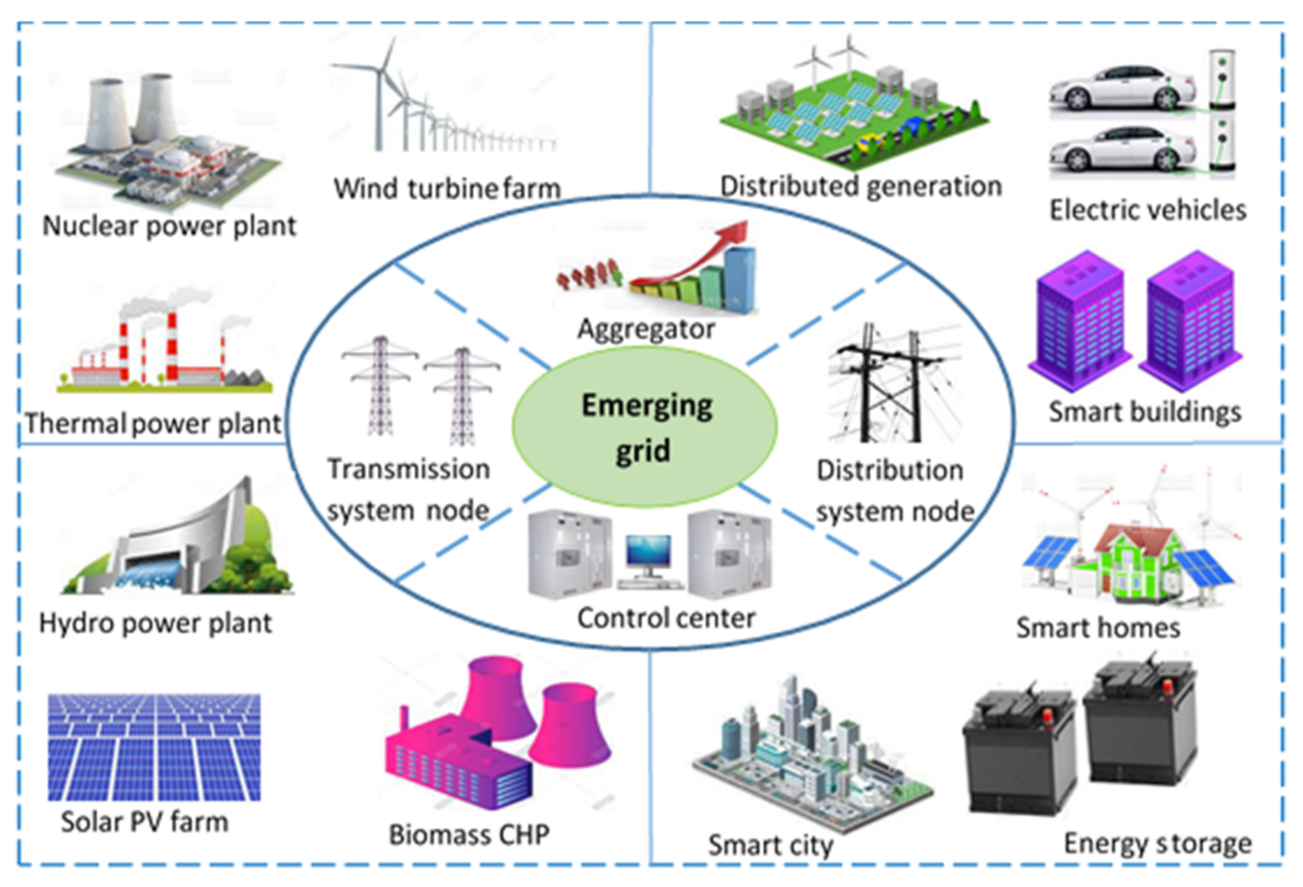
Figure 1 shows the emerging power grid with several components related to the generation, control, and utilization of energy. These components may be categorized into smart generation, smart transmission, smart distribution, and smart communication systems [2]. The smart generation is strongly linked to decarbonization and digitalization since the grid will contain a mix of large and small RES-based generation units. The smart generation also includes the microgrid model where active customer (prosumers) generates power through the distributed generation together with storage systems and transfers the surplus power generated to the grid [3]. The smart distribution system is based on the adoption of advanced distribution management technologies that will help optimize distribution network operations and increase network resiliency. The use of smart meters is also critical for energy usage monitoring and management. Smart distribution is the most recent notion, and it entails putting in place managerial measures. Smart distribution’s most recent concept is the use of managerial strategies to develop resources on the demand side by influencing load demand. The goal of smart communication systems is to eliminate information asymmetry and hence improve supply reliability. Power line communication technology, which allows bi-directional communication over existing power lines, is a key technology to achieve this goal [4].

System security has been defined by system regulators and operators for decades as the ability of a grid to withstand sudden changes in load and disturbances such as short circuits or unexpected network elements losses due to natural causes. Under this definition, the grid’s security can be evaluated under static security through voltage and thermal limits and under dynamic/transient security through voltage, angular, frequency stability studies [5]. The assessment of grids’ security under the impact of disturbances and unexpected network elements losses using these limits and stability studies may be regarded as a conventional security assessment. However, in modern grids with several Internet of Things (IoT) devices and wide area network controls, the focus of security assessments has been expanded to include cybersecurity assessment of the cyber-physical grid. The assessment of the cyber-physical grid security includes estimating the impacts of feasible cyber-physical attacks, evaluating the grid’s dependency on its cyber infrastructure, and assessing the ability of the grid to tolerate potential failures due to the cyberinfrastructure [6]. Comprehensive security assessment for the modern grid will be performed under the conventional security and cybersecurity assessments. However, the security state of the grid due to the impact of either the traditional disturbances or cyberattacks remains classifiable into the secure, insecure, and asecure states as given by Dy Liacco [7].

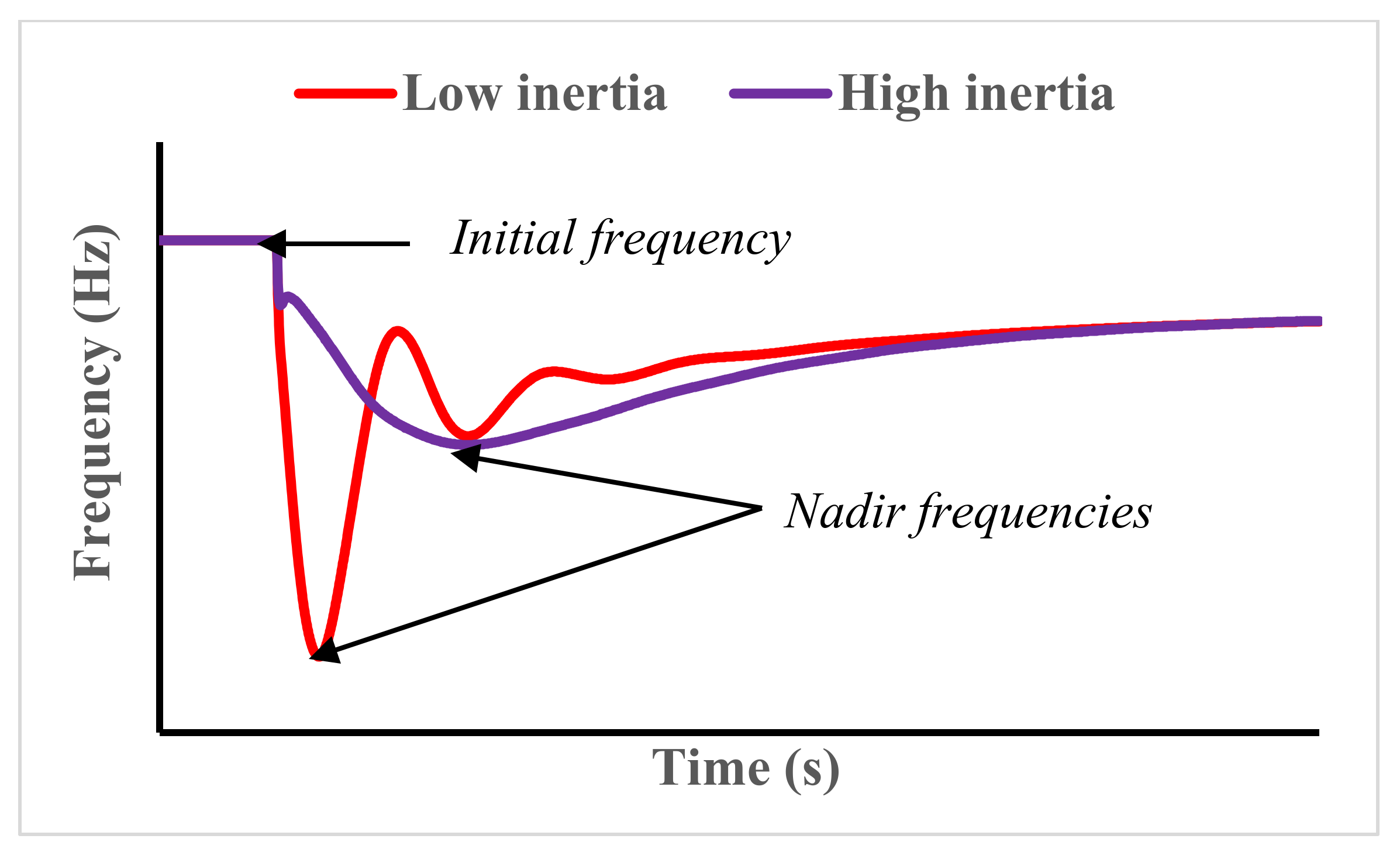
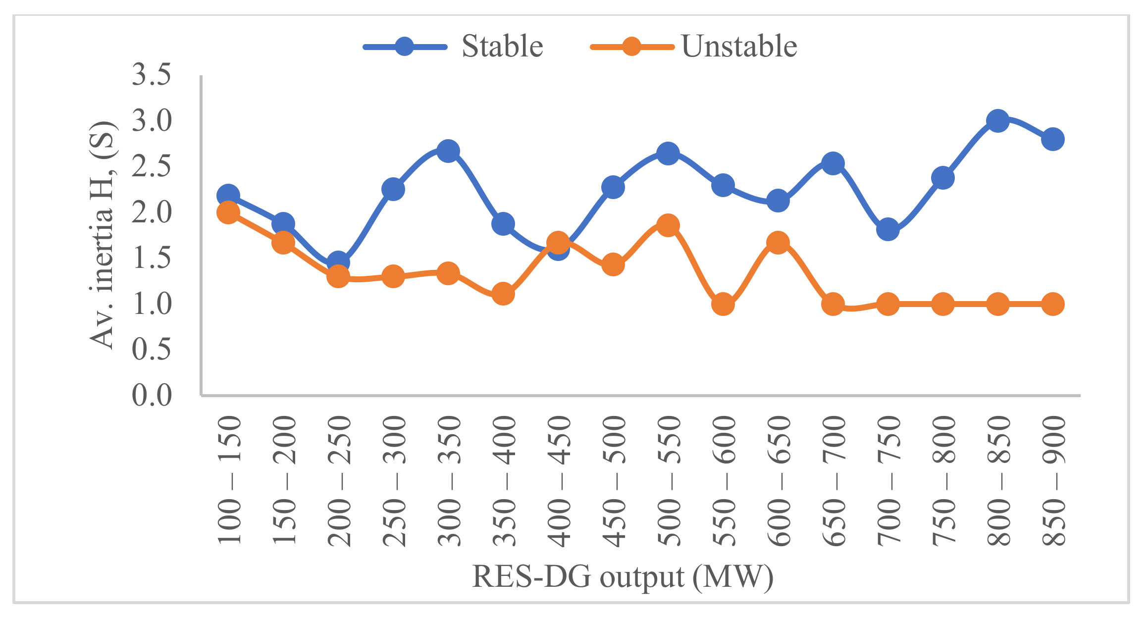
As more renewable energy sources distributed generation (RES-DG) units are added to the grid, the existing synchronous generators are disconnected and decommissioned. Since the RES-DG units do not provide any significant mechanical inertia to the grid, the grid’s resultant inertia constant is therefore notably reduced under high penetration of RES-DG units [8]. At reduced inertia, the steady-state operation of the grid may be secure since the disturbance is usually small and gradual. However, during fault conditions and large changes in load, the security of the grid may not be guaranteed. The insecure state is consequential to the grid not having sufficient inertial energy to withstand the perturbation during the period of the fault or large change in load. In addition to the inertia constant challenge, the reliability of the grid at high penetration levels of RES-DG units may be compromised due to the variability and intermittency of the power generation from the RES-DG units [9].

The deployment of data acquisition devices within the grid enables the generation of enormous data related to the state of the grid. Recent research focused on the application of machine learning techniques to identify patterns within the generated data to predict the security of the grid. Machine learning techniques are basically of two types, batch, and incremental learning techniques. In a real life application environment, machine learning is implemented as a repetitive process. A trained model is obtained using an appropriate algorithm on a preprocessed training dataset. If model performance is satisfactory, predictions of the class of new instances from the test dataset can then be obtained using the trained model [10]. The old (training) and the new (testing) datasets may then be combined to generate a new and larger dataset. Under the batch machine learning process, the predictive model needs to be retrained using the new and larger dataset. The performance of the latest model does not depend on the former model [11].

With the rapid deployment of data acquisition devices, the modern power grid will continue to generate a large amount of data in short time intervals. The models developed from the batch training modes are often discarded when a new model is obtained. There are several challenges associated with developing a batch machine learning model from a large dataset considering the continual increase in the dataset volume. To begin with, the time required in retraining a model from the combination of the old and new datasets is increased. The training time is proportional to the volume of the data. Consequently, the time lost between model retraining and deployment impacts the model user experience. In addition, the challenge of large memory requirements for the storage of the data for future applications will also be considered. The incremental learning process provides a solution to these challenges [12]. With batch training algorithms, the obtained classification model is seamlessly updated with new instances. The capability to effortlessly update the incremental machine learning models makes them more suitable for real life and online applications [13].

Many security prediction and control strategies have been proposed for the grid with and without considerations of the penetration of RES-DG units. One of the recent strategies is the application of a suitable machine learning algorithm to the existing dataset containing the historical security information of the grid. These machine learning-based prediction techniques were implemented in [14,15,16,17]. These techniques have shown their effectiveness to predict the security of the grid in case of transient security [14], frequency deviation [17], and distance to insecurity [18], without considering the penetration of any type of distributed generation into the grid. The techniques were based on only one system variable (voltage [14,15,16,18], frequency [17]). Considering the grid with high penetration of RES-DG, the proposed techniques may not be applicable under changing inertia and system loading. Batch machine learning-based techniques were proposed in [19,20]. Batch models may not be effective for real-time security prediction considering the time required to retrain the model when new data is available. For real-time security prediction capability, an incremental model that requires less amount of data for initial training is more effective.

Many existing models and techniques for security control in recent literature are based on restorative actions aimed to restore the system from the unstable to the normal state. Cases of implementation of primary and secondary frequency controls have been are presented in [21,22,23,24]. Models based on virtual power plant (VPP) application were proposed in [25,26]; synthetic inertia techniques were developed in [27,28]; and fast frequency response (FFR) control methods using backup generators were proposed in [29,30]. The VPP and FFR controls require complex algorithms, which are made more difficult by the significant penetration of RES-DG in the grid.

Considering the existing methods for under-frequency control due to the substantial variance in generation and load, demand-side contribution with load shedding has been effective to ensure quick system recovery grids frequency [31,32]. To estimate the load shedding required for frequency recovery, conventional analytical and optimization techniques [33,34,35], adaptive techniques [36,37], and meta-heuristic techniques [38,39] have been proposed. Although the existing methods can estimate and predict, to a reasonable degree of accuracy, the amount of load shed required to ensure the security of the grid through frequency control, the determination of the optimal load shedding nodes was not discussed. Also, most of the existing techniques are developed based on the relation of the grid’s power imbalance, the rate of change of frequency (ROCOF), and the frequency nadir. Therefore, the applicability of the techniques to a grid under varying attributes is highly doubtful. Furthermore, as synthetic inertia techniques for supporting conventional inertia in low inertia grids become more popular [40], it is necessary to anticipate the security of the grid for a specific level of inertia.

Table 1. Literature review summary.

References	Main Objective	Approach	Main Security Predictor (s)
[16]	Short-term voltage stability online prediction	Online	Voltage magnitude
[14]	Transient stability prediction	Offline	Rotor angle
[19]	Framework for transient stability prediction	Offline	Rotor angle
[41]	Prediction of the transient Stability Boundary	Offline	Voltage magnitude and rotor angle
[42]	Static security assessment	Offline	Voltage magnitude
[43]	Security assessment for multiple contingencies	Offline	Voltage magnitude
[7]	Power systems security assessment	Offline	Voltage magnitude
[15]	voltage stability prediction	Online	Voltage magnitude
[44]	Online static security Assessment	Online	Voltage magnitude and angle
[45]	Online transient stability prediction	Online	Voltage magnitude and rotor angle

shows a summary of existing techniques in recent literature for the security assessment and prediction of a power grid.

Security predictors in existing frameworks and techniques have largely been determined by changes in system load and generation. These determinants are effective for conventional grids with insignificant penetration of non-synchronous generators. However, to achieve effective security prediction for the modern and emerging grid, there is a need to extend the predictor determinants to include varying parameters critical to the grids with high penetration of non-synchronous generators. Consequently, it is important to develop a method to achieve fast security prediction and control that takes into consideration changes in inertia, generation levels from renewable energy systems, and network contingencies. Hence, the contributions of this paper include:

• demonstrating the feasibility of security prediction using a time-varying system’s deterministic and probabilistic attributes,
• developing a model using an incremental Naïve-Bayes algorithm for online security prediction for the emerging grid,
• proposing a gaussian process regression load shed estimation method to ensure the security of the predicted insecure network operation instances and,
• proposing a voltage security index ranking technique for optimal load shed node(s) selection.

This paper is focused on the emerging grid with variable penetration levels of RES-DG units that will result in varying inertia constants of the grid. The proposed model is based on an incremental Naïve Bayes classification algorithm for security prediction based on the rotor angle response obtained from the transient stability assessment of the network to a three-phase short circuit fault. The attributes considered for the classification are inertia constants, the system loadings, the RES-DG power generation, and the fault location within the grid. An additive Gaussian process regression (GPR) model using the Pearson Universal kernel (PUK) is developed to estimate the amount of load shed required to ensure the security of the insecure predicted network instances. In conclusion, the suitable node (s) for the load shedding is determined using a ranking algorithm based on the node loads and voltage security margins.

The rest of this paper is organized as follows. Section 2 discusses the impact of high penetration of RES-DG units on the power grid as well as the security modeling and assessment of the integrated transmission and distribution network considering time-changing inertia. Online machine learning with the proposed incremental classification algorithm and intelligent security control are presented in Section 3. 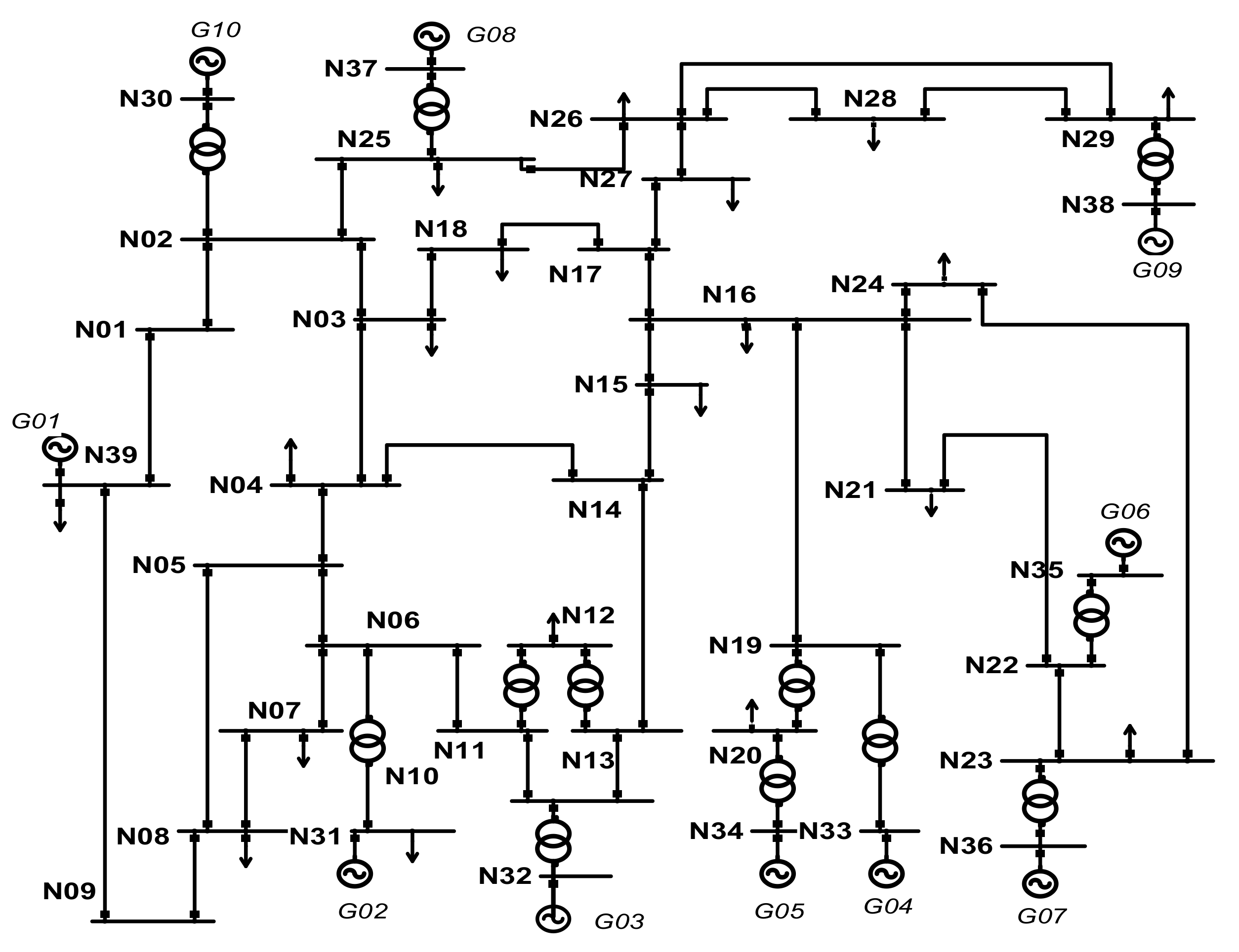Section 4 contains the results and discussions obtained from testing the proposed techniques on the IEEE 39 bus network, while the conclusions are presented in Section 5.

2. System Security and Inertia Constant Modelling

2.1. RES-DG Units and Time Changing Inertia

More fossil fuel-based synchronous generators will be made redundant as the penetration of RES-DG units increases. The RES-DG units are connected to the grid through electronic converters, therefore, they do not supply mechanical inertia to the grid. The frequency of the power grid is controlled by the inertia supplied by synchronous generators within the grid. At low penetration of RES-DG into the grid, the frequency response may not be significantly impacted. However, as the RES penetration level increases, frequency stability and power oscillations within the grid under disturbances becomes a challenge. Attempts have been made to estimate the instantaneous RES-DG penetration level beyond which the grid frequency may fall below the security range after a disturbance.

Traditionally, the inertial response from the synchronous generator is an inherent characteristic, and it is not treated as an ancillary service. However, with the increase in penetration of RES-DG, the grid operators in several power systems have identified inertia as an ancillary service [46]. From the grid operator’s perspective, the grid can be categorized as a high and low inertia grid depending on the penetration level of RES-DG. A grid with low penetration of RES-DG is referred to as a high inertia grid, and a grid with a high penetration of RES-DG is described as a low inertia grid. Figure 2 shows the frequency responses of the grid under high and low inertia values. Under low inertia values, the Nadir frequency and the rate of change of frequency (ROCOF) are both increased. Also, more oscillations are experienced by grids with low inertia values before attaining stability.

Considering the rapid proliferation of RES-DG units into the grid, it is therefore important to be able to predict the security of the grid under changing inertia values. The equivalent inertia constant ($H_{eq}$) for a grid at a particular time can be derived as shown in Equations (1) and (2).

$$H_i=\frac{E_k}{S_{r,i}}$$

(1)

$$H_{eq}=\frac{{{\displaystyle \sum }}_{i=1}^N{H}_i\times S_{r,i}}{S_B}$$

(2)

where $H_i$ is the inertia of the $i-th$ synchronous generator, $S_{r,i}$ is the rated apparent power of the $i-th$ synchronous generator, $E_k$ is the total rotational kinetic energy stored in the grid, $S_B$ is the base power of the grid, and $N$ is the total number of synchronous generators connected to the grid.

2.2. Power System Security Modeling and Assessment

System security is defined as the ability of the system operating point to remain within the secured zone in which any of the constraints are not violated under dynamic and transient conditions [47]. According to IEEE standard 1547.1-2015 [48], the operation of RES-DG units within a grid should not result in the insecurity of the grid. Consequently, at high penetrations of RES-DG, the grid should be able to remain in a secure state during and after the occurrence of contingencies. Any constraints violations leading to insecurity during and after the occurrence of a contingency should be confined to an area within the grid. The constraints under which the security can be assessed are developed based on the system variables of concern. As shown in Figure 3, variables a, b, c, and d represent the node voltage, rotor angle, frequency, and current limits for the $i-th$ operating point for the system under a contingency. The $i-th$ operating point is represented by the dots along the trajectory of each variable at a specific time. The operating points represented by the different coloured dots move from the secure state (green colour) to the insecure state (red colour). Depending on several factors, including the type of contingency, a network may have operational points in different security states at the same time. However, it is common to have the system variable operating points existing in the same security state.

As stated earlier, the security state of a network may be assessed using several network variables including the post contingency voltage and frequency values as well as the rotor angle response of the synchronous machines. During contingencies, the values of network variables are allowed to deviate over a specified security limit. However, to achieve a new security state, the grid’s frequency and voltage must return to the initial values while the rotor angle settles at a new stability point. The security of the grid largely depends on the dynamic parameters of the generators, transmission system, and load. The general steps to security assessment include contingency screening, contingency ranking, and security assessment using appropriate indices.

2.3. System Modeling for Transient Stability Assessment

A disturbance within a grid caused by a fault or sudden change in load leads to the exchange of stored kinetic energy between the system’s synchronous generators. The result is a change in the speed of each generator. Since the change is different for each generator, the generators swing relative to each other and relative to the reference generator in the grid causing the flow of synchronizing power among the generators. Faults within a section of the grid create large disturbances within the boundaries of such grid section. The fault may be due to but not limited to equipment malfunction, human errors, natural disasters, and attacks. The effects of the disturbances may spread across the whole grid if quick action is not taken. It is, therefore, the responsibility of the grid operators to ensure the reliability of the power supply considering the possibility of disturbances.

The general model used to ensure reliability is to anticipate and assess the fault conditions through transient security studies, and implement appropriate methods to limit the impact of the disturbances. The model of the power grid is based on the synchronized operation of several generators connected in parallel within the grid. If the synchronization criteria are met, generators can be readily added and removed, depending on the situation of the grid. To elaborate, the degree of security of the grid depends on the size of the generators, the locations of the generators within the grid, the transfer capacity of the transmission network, the load distribution, and the type of disturbance.

The relative swinging of the synchronous generators to each other and the reference generator is due to the non-uniformity in sizes and other dynamic parameters such as the inertia constant. Synchronism is lost when the swing of one or more synchronous generator(s) is beyond control; hence, the generator is said to be out of step. To avoid grid collapse, the out-of-step generator must be swiftly disconnected from the grid through the protection devices. The ability of the system to remain in synchronism after the occurrence of a fault is assessed under transient security studies. Considering the dynamic model of the synchronous machines, the grid can be represented by differential-algebraic equation models in (3) to (5) using the $d-q axis$ model [49].

$$T_{doi}^{\prime }\frac{d{E}_{qi}^{\prime }}{dt}=-E_{qi}^{\prime }-\left(X_{di}-X_{di}^{\prime }\right)I_{di}+E_{fdi}$$

(3)

$$T_{qoi}^{\prime }\frac{d{E}_{di}^{\prime }}{dt}=-E_{di}^{\prime }+\left(X_{qi}-X_{qi}^{\prime }\right)I_{qi}$$

(4)

$$T_{avi}\frac{d{E}_{fdi}}{dt}=-E_{fdi}+K_A\left(V_{ref}-V\right)$$

(5)

where $T_{di}^{\prime }$ and $T_{qi}^{\prime }$ are the open-circuit time constants in the d and q axis, respectively; $E_{di}^{\prime }$ and $E_{qi}^{\prime }$ are the d-axis and q-axis transient voltages; $X_{di}$ and $X_{qi}$ are the $d$ and $q$ synchronous reactances; $X_{di}^{\prime }$ and $X_{qi}^{\prime }$ are the d and q transient reactances; $E_{fdi}$ is the excitation system voltage; $I_{di}$ and $I_{qi}$ are the $d$ and $q$ armature current, respectively; $T_{avi}$ is the voltage regulator time constant; $K_A$ is the voltage regulator gain; $V_{ref}$ is the reference voltage; and $V$ is the generator terminal voltage. If ${\omega }_i$ is the $i-th$ synchronous generator rotor angular speed, ${\omega }_s$ is the synchronous angular speed of the grid, $P_m$ is the synchronous generator mechanical power, and $P_e$ is the synchronous generator electrical power, then the rotational dynamics of the synchronous generators’ rotor is given by Equations (6) and (7).

$$\frac{d{\delta }_i}{dt}={\omega }_i-{\omega }_s$$

(6)

$$\frac{2H_i}{{\omega }_s}\frac{d{\omega }_i}{dt}=P_m-P_e-D_i\left({\omega }_i-{\omega }_s\right)$$

(7)

where ${\delta }_i$ is the rotor angle of the $i-th$ synchronous generator. If $R_{ai}$ is the armature resistance, then the synchronous generator stator can be modeled using the algebraic Equations given by (8) and (9).

$$E_{qi}^{\prime }-V_{i}cos\left({\delta }_i-{\theta }_i\right)-R_{si}{I}_{qi}-X_{di}^{\prime }{I}_{di}=0$$

(8)

$$E_{di}^{\prime }-V_{i}sin\left({\delta }_i-{\theta }_i\right)-R_{si}{I}_{di}-X_{qi}^{\prime }{I}_{qi}=0$$

(9)

3. Online Security Prediction

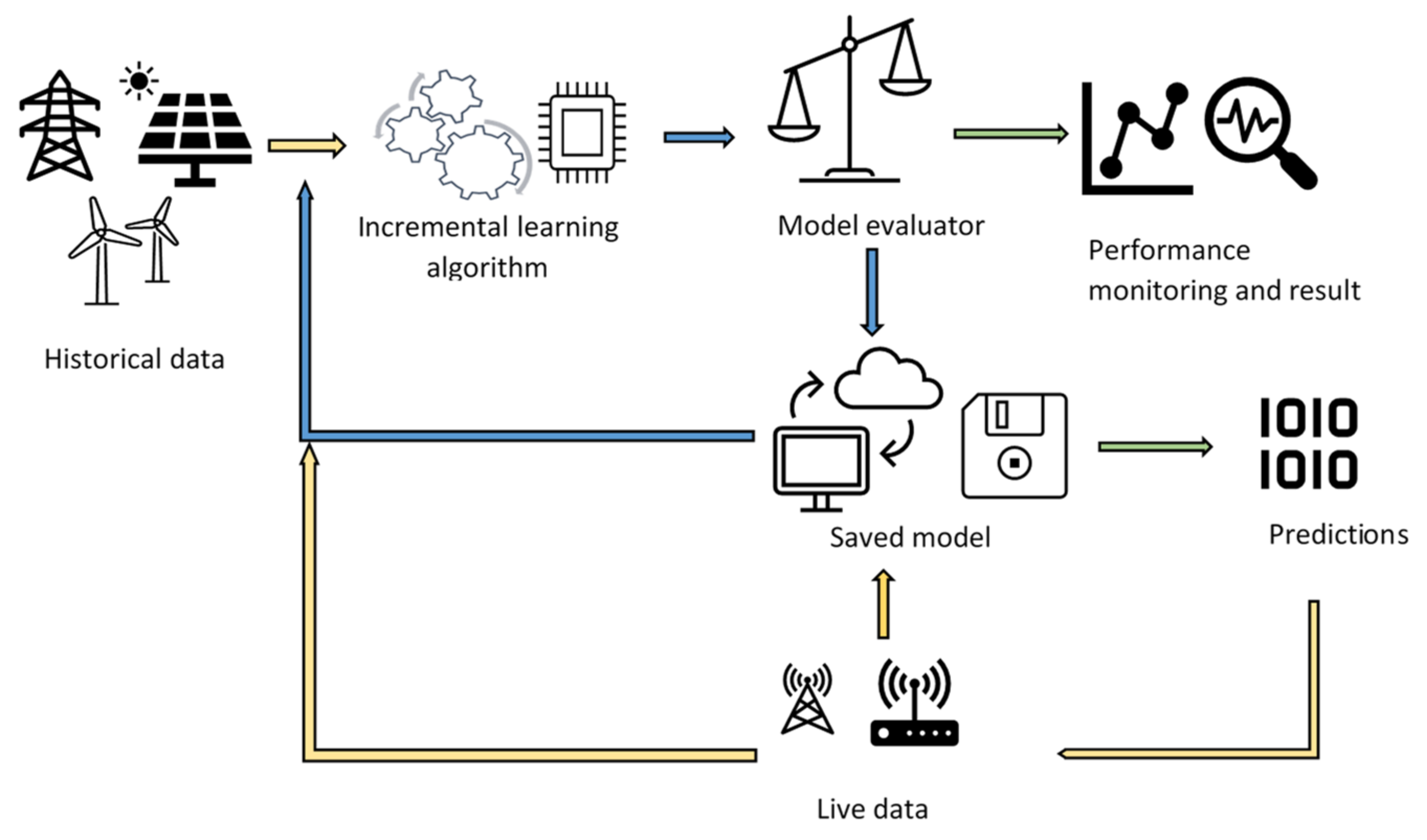
This section describes the steps involved in the development and deployment of an online machine learning model. As shown in Figure 4, historical training data is obtained through recorded real-life operations and responses to significant events such as three-phase short circuit fault. Historical training data can also be represented by the responses of the network to several transient stability simulation scenarios using an appropriate simulation tool. The training dataset is then preprocessed to determine attribute suitability and impact on security (class of dataset) through filtering and/or correlation. A suitable machine learning algorithm is selected and then applied to the training dataset. The suitability of an algorithm for a classification model depends on several factors that include the data types, storage availability, and type of training (batch or incremental). The step-by-step operation of an online prediction model is shown in Figure 4. Since the model in the paper is intended for online security prediction, this paper focuses on the incremental Naïve Bayes classification algorithm.

The performance of the incremental model is evaluated at each training step. In a classification problem, a model with high accuracy ($\alpha$) and low misclassification rate ($\beta$) is desirable. If $N_c$ is the total correctly classified instances in the stream of the dataset, $N$ is the total instances in the stream of the dataset, $N_m$ is the number of misclassification in the $k-th$ and $Nk$ is the total number of instances in the $k-th$ class [45], then the accuracy and misclassification of a model can be evaluated using Equations (10) and (11).

$$\% \alpha =\frac{N_c}{N}\times 100$$

(10)

$$\% \beta =\frac{N_m}{Nk}\times 100$$

(11)

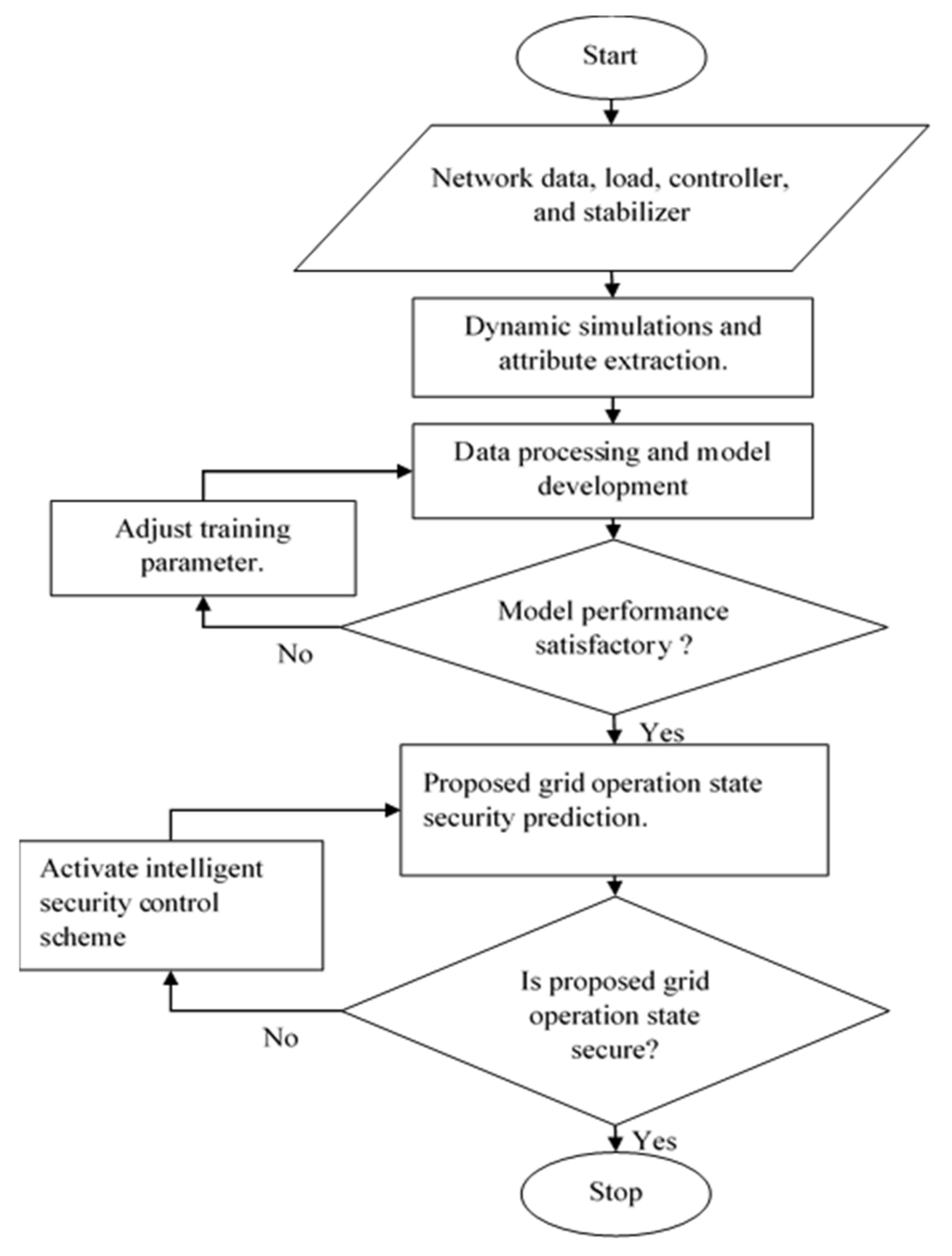
The approach proposed in this paper involves transient security assessment under varying system parameters and grid operation points. The methodology proposed in the section above is focused on the prediction of the security of the grid for a given grid operating point. The knowledge of the security state of the grid using past and present data is required to determine techniques to ensure the security of the grid. The steps for the online security prediction and control technique proposed in this paper are described in the flowchart in Figure 5. The integrated transmission and distribution network is modelled with a suitable automatic voltage regulator, power system stabilizer, and governor control for transient stability assessment with the necessary controllers for the RES-DG units. Transient stability assessment is performed on the grid to determine its response to three-phase bolted fault. The transient security assessment is performed several times using varying network parameters and grid operation points to obtain instances for the training dataset. The variable network parameters and grid operation points are regarded as the attributes of the training dataset and include the equivalent inertia constant, the load level, the aggregated RES-DG units output, and the fault distance. To optimize the model’s accuracy and performance, the incremental Naïve-Bayes based-model training is carried out using the continual learning approach. With continual learning, the model can autonomously relearn from a stream of data and adapt automatically as new data is available to improve accuracy and performance.

The continually trained model is saved after the best obtainable accuracy is obtained. The obtained Naïve Bayes security prediction model is ready for deployment at any stage of the training between each data streams. If the security state prediction of the model to a proposed system operating state (live data) is correct, the predicted security state with the system operating state is afterward considered as historical data and used to improve the performance of the model. For the predicted insecure states, a regression-based model is proposed to estimate the amount of load shed required to ensure the security of the grid. Also, an algorithm to determine the optimal node for load shedding is proposed.

3.1. Online Machine Learning Model Development

Online security prediction is the response to system operation state given the knowledge of the true security state of previous operation states and, possibly, the availability of additional information. Online prediction models imitate the ability of humans to give responses and make rational decisions in an intelligent and programmed manner using basic everyday attributes. An online prediction model is used to predict the outcome of successive instances. In this paper, a binary classification model to predict whether the grid is secured or not using specific grid attributes is proposed. After the proposed grid event (instance), the true security response is received as feedback from the grid. Using this feedback, the difference in the precision of the prediction and the true security state can be measured. Based on the precision difference, the model is updated to improve predictive performance for future predictions. If $w$ is the classification model and $N$ is the number of training rounds for the model, then the steps for the development of an online binary classification model can be summarized as below [50]:

• Initialize the prediction function, $F_1$,
• Receive new instance: $x_t\in R$; where $t=1, 2, 3\dots T$,
• Predict class $y_t=F_t{X}_t,$ for $x_t$,
• Obtain true class label: $y_t{}^{*}\in \left\{secure, not secure\right\}$,
• Measure the loss suffered: $l_t\left(F_t\right)$,
• Update model from $w_t$ to $w_{t+1}$.

The number of classification mistakes made by online learning algorithm can be measured using Equation (12). The performance of an online algorithm is measured by the cumulative loss it suffers during the run of the $T$ sequences. The objective of the online learning task is to minimize the regret function of the model’s predictions against the best-saved model before the present prediction task as defined in Equation (13). Assuming that the true responses are generated by an unknown but fixed hypothetical factor $g$ such that $y_t=g(x_f)$ for all $t\in T$ the cumulative loss of $g$ over an entire sequence is zero and is independent of $T$. The loss function in this paper is formulated as an online convex optimization (OCO) problem with respect to $w$ and is defined as Equation (14)

$$M_T={\displaystyle \sum }_{t=1}^T\left(y_t{}^{*}\ne y_t\right)$$

(12)

$$R_T={\displaystyle \sum }_{t=1}^T{l}_t\left(w_t\right)-\underset{F}{\min }{\displaystyle \sum }_{t=1}^T{l}_t\left(w\right)$$

(13)

$$f_{c-t}=l\left(g_w,\left(x_t,y_t\right)\right)$$

(14)

where w is the classification model, and $l_t$ is the loss suffered by the optimal model. It is important to note that $w_t$ can only be known after the examination of all the instances and their class labels.

3.1.1. Incremental Naïve Bayes model

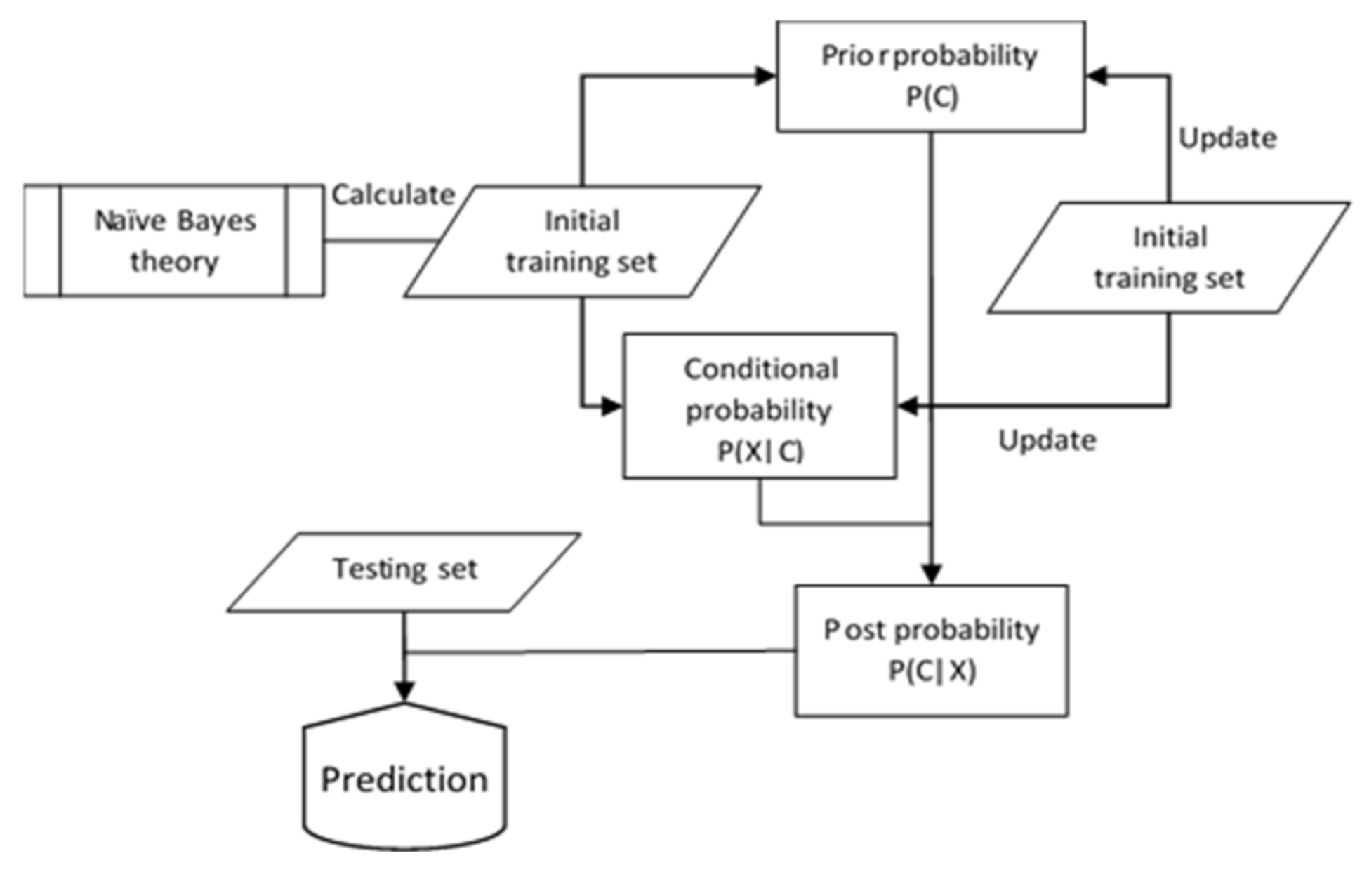
The incremental Naïve Bayes algorithm is used to realize the online classification model in this paper. The basic idea of the incremental Naive Bayes algorithm is to calculate a posterior probability based on the prior probability and new data [51]. The ability of the incremental Naive Bayes classification algorithm to support online learning is due to its leverage on and exploitation of prior information of the datasets. The structure for the incremental Naïve Bayes algorithm is shown in Figure 6. The posterior probability is estimated from the prior probability and existing data. The predicted posterior probability will then become the new prior probability for the next learning batch [52,53]. Subsequently, the incremental learning algorithm saves the updated prior probability as knowledge. To achieve unification of knowledge when new data is received, incremental learning algorithms estimate a new knowledge for the new data based on the old knowledge. The classification accuracy and precision are improved by adjusting the prior probability.

The post probability $P(C|X)$ is the probability of an instance belonging to class $C$. The conditional probability $P(X|C)$ is the likelihood of a specific class occurring, based on the occurrence of a previous instance. The class prior probability $P\left(C\right)$ is the estimate of the probability that a randomly sampled instance from a dataset will yield a given class notwithstanding the attributes of the instance. If $X=\left[A_1, A_2,\dots , A_n\right]$ is a sample dataset with $n$ attributes, then the post probability from the traditional Naïve Bayes principle can be evaluated using Equation (15).

$$P\left(C|X\right)=\frac{P(X|C)P\left(C\right)}{P\left(X\right)}$$

(15)

If $C_1, C_2,\dots , C_m$ denotes the $m$ different possible classes, then for each dataset $X$, the post probability $P(C_j|X)$ is evaluated using the prior probability $P\left(C=C_j\right)$ and conditional probability $P(X|C_j)$ as given in Equation (16).

$$\frac{P(X|C_i)P\left(C_i\right)}{P\left(X\right)}>\frac{P(X|C_j)P\left(C_j\right)}{P\left(X\right)}$$

(16)

where $P\left(C_i|X\right)>P\left(C_j|X\right)\dots \dots 1\le i\ne j\le m$.

From Figure 6, it is shown that the process of updating the incremental learning of the Naïve Bayes classifier is a recursive Bayesian estimation of parameters. Its advantage is that information in initial training data is preserved in the form of parameters. During the incremental learning process, the initial training data can be discarded to conserve memory since the information contained in the initial training set has been stored in the form of two key statistic parameters: the class prior probability and the conditional probability. Suppose $X^{*}$ is the new testing dataset and $X^{*}={\left[A_1, A_2,\dots , A_n\right]}^{*} \in M$ are the new instances for updating the prior and conditional probabilities, then the model for updating the class prior probability is given in Equation (17).

$${\phi }_j=\left\{\begin{array}{l}\frac{\tau }{\tau +1}{\phi }_j+\frac{1}{1+\tau } when C_d=C_j\\ \frac{\tau }{\tau +1}{\phi }_j when C_d\ne C_j\end{array}\right.$$

(17)

where $C_d{}^{*}$ is the class label, ${\phi }_j=P\left(C=C_j\right)$ is the class prior probability of class label $C_j$, $\tau =n+m$, $n$ is the number of instances in the initial training set $N$ and $m$ is the number of instances in the new training dataset $M$.

The performance of incremental Naïve Bayes models is assessed using specified metrics, similar to the traditional Naïve Bayes models. Generality, accuracy, learning rate, classification costs, and storage requirements are some of the common metrics. This paper, however, focuses on the accuracy evaluation metrics that can be expressed using the precision ($Pre$), recall ($Rec$), and F measure ($Fm$) as shown in Equations (18)–(20). The precision of the model is the proportion of the predicted security state from the dataset that is correct, the recall is the proportion of the dataset that is correctly classified. Occasionally, the precision or recall may not truly represent the properties of a model. Consequently, the F-Measure is employed to combine the recall and precision into a single metric that effectively captures the performance of the model as given in Equation (21) [54].

$$ACC \left(\%\right)=\frac{TN+TP}{\left(TN+FN+FP+TP\right)}$$

(18)

$$Pre \left(\%\right)=\frac{TP}{\left(FP+TP\right)}$$

(19)

$$Rec \left(\%\right)=\frac{TP}{\left(FN+TP\right)}$$

(20)

$$Fm \left(\%\right)=\frac{2Pre \times Rec}{Pre+Rec}$$

(21)

where TP (true positive) is the number of correct predictions that an instance is relevant, TN is the number of correct predictions that an instance is irrelevant, FP (false positive) is the number of incorrect predictions that an instance is relevant, and FN (false negative) is the number of incorrect predictions that an instance is irrelevant.

3.1.2. Implementation for Real-Time Security Prediction

The dimensionality and types of attributes of the dataset determine the feasibility of real-time applicability. Using the incremental learning technique, highly dimensional large training datasets are reduced into small dataset batches. In this case for power system real network application, security predictions are made for a single instance as obtained from field devices such as PMU, therefore, the prediction time is diminutive. The situation that may be regarded as a challenge is the speed at which the saved incremental classifier can be retrieved from the different storage means.

There are several artificial intelligence application development tools for implementing incremental learning approaches. However, only a few tools support online applications. Weka software is one of the few tools that provides an online machine learning application development environment [51]. In particularly demanding real-world applications like security state prediction for the grid operators, the Weka environment can be used to produce real-time predictions. On Weka, many classifiers can be trained and implemented using the incremental mode. However, training classifiers on large datasets can be challenging even after reduction into smaller batches, particularly using the Weka explorer interface.

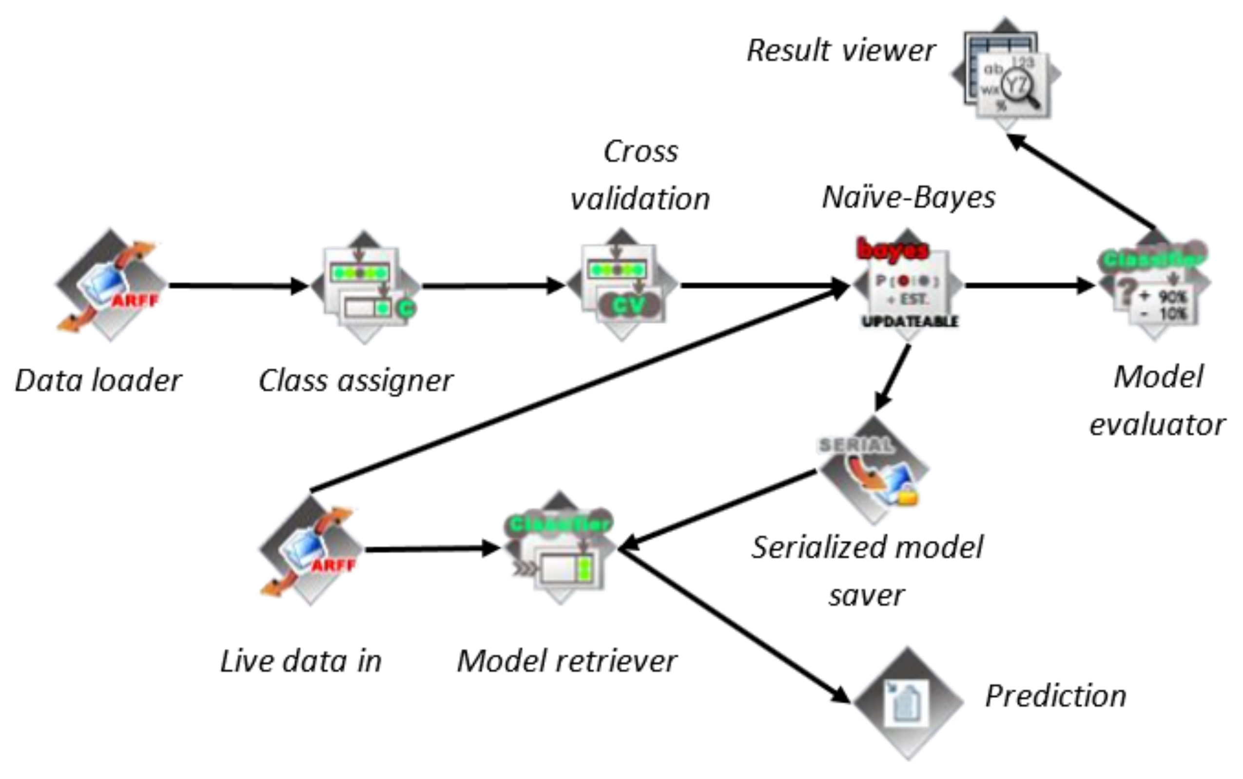
In the Weka explorer interface, due to the visualization and other functionalities, the computer’s memory may be overloaded, which may significantly impact the training and prediction times. An alternative to the graphical user interface is the Knowledge Flow interface. The knowledge flow layout showing the important steps and elements for the proposed set-up is shown in Figure 7. The knowledge flow interface makes it possible to process large datasets that would have significantly impacted the computer’s processing speed. By loading and processing each instance in a dataset separately, updateable classifiers may be trained incrementally. After each successful training, the serialized model saver saves the most recent model, which is then retrieved by the model retriever to make future security state predictions using live data.

3.2. Intelligent Security Control System

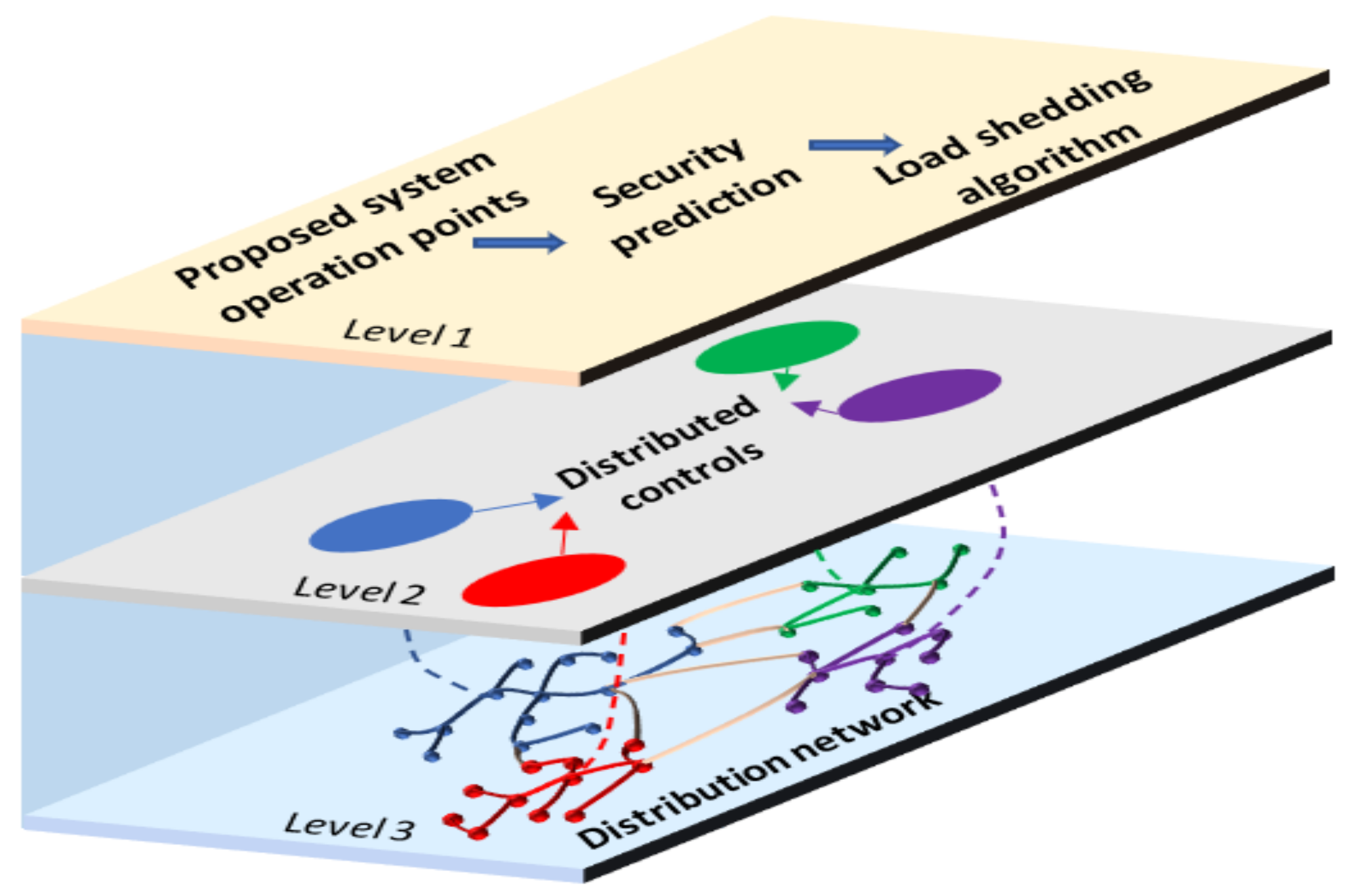
An intelligent security control (ISC) system based on load shedding is proposed to ensure the security of the grid for predicted insecure states. The ISC system determines the secured load level for an insecure state, estimates the required load shed value, and determines the best node within the network for load shedding action. The ISC system model is developed from a dataset of proposed grid operating points with a new load and simulated response from the offline transient security studies. A load shed value for an insecure proposed grid operation point is estimated to ensure grid security by constantly monitoring the output of the security prediction model. The proposed ISC system is implemented on the physical distribution network through the distributed controls enabled by communication devices as shown in the modern grid structure in Figure 8. The proposed security prediction and ISC model exists on the first layer of the integrated grid structure. Layer 2 comprises distributed control systems for different zones of the distribution network. Commands from the ISC are implemented to activate the necessary switches in sections of the distribution network on layer 3 of the integrated transmission and distribution network structure.

The development of the model for the ISC is achieved in two stages. In the first stage, the estimation of the amount of load shed to ensure the security for the predicted insecure state of the network is carried out. To estimate the load shed amount, an additive Gaussian process regression algorithm is applied to train the developed dataset. In the second stage, the optimal node for load shedding action is determined using a ranking algorithm based on the network node’s security margin.

3.2.1. Gaussian Process-Based Load Shed Value Estimation

This section describes the proposed algorithm to estimate the amount of load shed required to ensure the security of the grid for all predicted insecure states. A new dataset containing the new loads’ values for every insecure instance from the initial dataset is developed. An additive Gaussian process regression (GPR) prediction algorithm is proposed to predict the secured load level for insecure predictions from Section 3.1. GPR is a nonparametric Bayesian approach with several benefits. A few of the benefits include the capability to work well on small datasets and the ability to provide uncertainty measurements on the predictions. A GPR is a generalization of the Gaussian probability distribution. It is a stochastic process in which a multivariate normal distribution exists for every finite collection of random variables. In other words, a normal distribution is assumed for any finite combination of variables.

Since the proposed load shedding model is described by more than one attribute $(x_1,x_2,\dots ,x_N)$ with high correlation to each other, the distribution of the attribute can be represented by a multivariate Gaussian distribution model defined in Equation (22).

$$\aleph \left(x|\mu ,\sum \right)=\frac{1}{2{\pi }^{N/2}{\sum }^{1/2}}exp\left[-\frac{1}{2}{\left(x-\mu \right)}^T{\sum }^{-1}\left(x-\mu \right)\right]$$

(22)

where $N$ is the dimension of the dataset, $x$ is the variable, $\mu$ is the mean vector, and $\sum$ is the $N\times N$ covariance matrix. Since it is possible to have a probability distribution function for all possible predictions in GPR, the means of the predictions, as well as the prediction variances, can be calculated. The multivariate regression prediction can be modelled as given in Equation (23).

$$P\left(f|X\right)=\aleph \left(f|\mu ,K\right)$$

(23)

where $X$ is the vector of attributes denoted by $X=\left[x_1, x_2,\dots , x_N\right]$, $f=\left[f\left(x_1\right), f\left(x_2\right),\dots , f\left(x_N\right)\right]$, $\mathrm{\mu }=\left[\tau \left(x_1\right), \tau \left(x_2\right),\dots , \tau \left(x_N\right)\right]$ and $K_{ij}=k\left(x_i,x_j\right)$, $\tau$ represents the mean function, and $K$ represents a positive kernel function. A kernel function is commonly used in GPR to represent the behavior of the dataset. The Pearson Universal Kernel (PUK) function expressed in Equation (24) is chosen due to its ability to adapt to various other functions [55]. The conditional densities and posterior for prediction are given by Equations (25) and (26), respectively. The GPR performance indices $\alpha$ and $\beta$ are given in Equations (27) and (28).

$$K\left(a,a_0\right)=\frac{1}{{\left[1+{\left(\frac{\sqrt[2]{{\left|a-a_0\right|}^2\sqrt{2^{\left(\raisebox{1ex}{$1$}\!\left/ \!\raisebox{-1ex}{$\omega $}\right.\right)}-1}}}{\sigma }\right)}^2\right]}^{\omega }}$$

(24)

$$\left[\begin{array}{c}p\left(x_1\right)=\aleph \left(x_1|{\mu }_1,{\sum }_{11}\right)\\ p\left(x_2\right)=\aleph \left(x_2|{\mu }_2,{\sum }_{22}\right)\\ p\left(x_3\right)=\aleph \left(x_3|{\mu }_3,{\sum }_{33}\right)\end{array}\right]$$

(25)

$$p\left(x_1|x_2\right)=\aleph (x_1|{\mu }_{1|2}, {\sum }_{1|2})$$

(26)

$$\alpha =IC{M}_{lv}\times \overrightarrow{TV}$$

(27)

$$\beta =IC{M}_{hv}\times \overrightarrow{TV}$$

(28)

where ${\mu }_{1|2}={\mu }_1+\sum \sum _{12}^{-1}\left(x_2-{\mu }_2\right)$, $a_0$ is the center of the peak of the kernel function, $a$ represents an independent variable, $\omega$ is used to control the Pearson width, $\sigma$ is the tailing factor of the function peak, $\overrightarrow{TV}$ is the vector of the target values, and $IC{M}_{lv}$ and $IC{M}_{hv}$ are the lowest and highest values of the inverted covariance matrix, respectively. To optimize the performance of the GPR model, the model is implemented using the additive function. An additive GPR is a function that decomposes into a sum of low-dimensional functions, each depending on only a subset of the input attributes. If the attribute-class pair is $(x_i, y_i)\in$ R^d × R, where $i=1, 2,\dots , N$ then the additive non-parametric GPR is defined as Equations (29) and (30) [56]

$$y_i=F({\mathrm{x}}_i)+{ϵ}_i, {ϵ}_i~N\left(0,{\sigma }^2\right)$$

(29)

$$F\left(x_i\right)={\phi }_1{f}_1\left(x_i\right)+{\phi }_2{f}_2\left(x_i\right)+\dots +{\phi }_z{f}_z\left(x_i\right)$$

(30)

where $N$ is the sample dimension, $d$ is the dimensions of $x_i$, $F$ is the sum of the $z$ regression function, and $\phi$ is the parameter that prevents $F$ from sample overfitting.

3.2.2. Optimal Node Selection

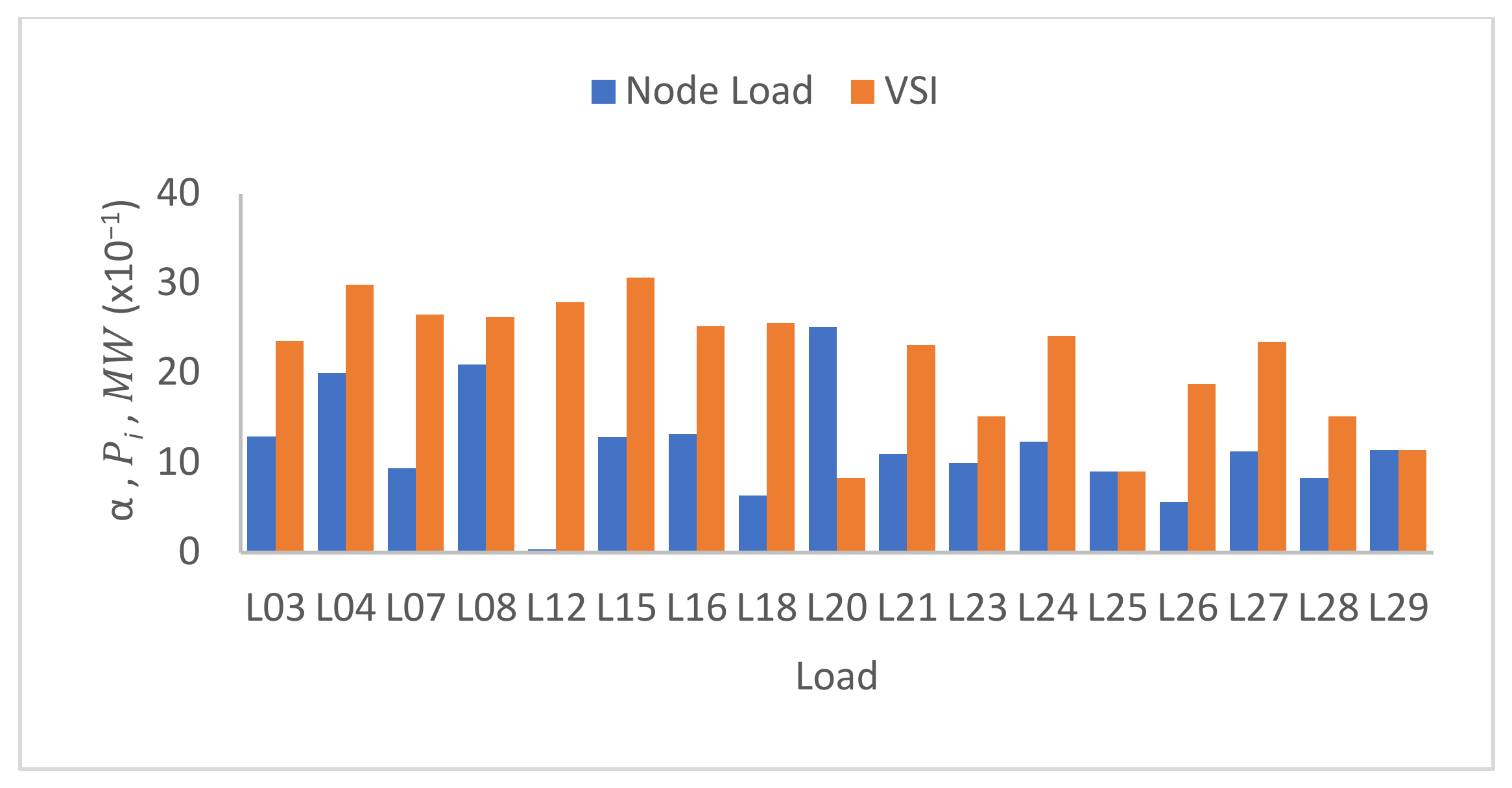
After estimating the load shed value required to ensure the security of the grid, the next step is to determine the appropriate node within the grid to apply the intelligent load shedding scheme. The proposed optimal node selection algorithm is based on the security margin of individual nodes within the network. Security margin is defined as the closeness of a node to insecurity, and is obtained from the critical voltage ($V_{cr}$) and the initial voltage ($V_{in}$). The $V_{cr}$ is the voltage at the point of collapse obtained from the voltage stability assessment for each node while $V_{in}$ is the initial voltage at the node. If $N$ is the total nodes in the network, the proposed algorithm for load shedding node identification is given below.

Model 1: Load shedding node(s) selection

• System initialization $i=1, 2, 3\dots N$.
• Read the node load $P\left(i\right)$ and required load shed value $P_{ls}$.
• Evaluate the node’s security margin $\alpha \left(i\right)$,

  $$\alpha \left(i\right)=\left(\frac{V_{in}\left(i\right)-V_{cr}\left(i\right)}{V_{cr}\left(i\right)}\right)\times 100.$$
• Sort $\alpha \left(\nabla \right)==\alpha \left(i\right)$ (largest $\to$ smallest).
• Initialize $i=1$.
• if $P\left(i\right) \left[\alpha \left(\nabla \right)\right]\ge P_{ls}$ then.
• $i$ is a load shedding node.
• else $i=i+1$.
• until $\sum _i^{n}P\left(i\right)\ge P_{ls}$.
• end
• return node(s), $i$.

4. Results and Discussion

4.1. Test Network

The proposed technique was tested on the IEEE 39 bus test network with 10 generators and 19 load buses as shown in Figure 9. The synchronous generators are modelled with the constant gain exciters and conventional power system stabilizers. Generator G3 is chosen as the center of inertia due to its lateral position with the grid. The network is reduced to a single machine infinite bus model and modified to include a non-synchronous generator at the lower voltage side. The wind turbine system is used to represent the aggregated power generation from renewable sources.

The network operation parameters considered for the transient security assessment are given in

Table 2. Parameter for Security Assessment.

Attributes	Value Range
Load (MW)	500–2500
Inertia Constant (s)	0.1–3.5
RES-DG output (MW)	100–1000
Fault distance (%)	10–100

. These parameters are also considered as the attributes in the training dataset to obtain the security prediction model. A three-phase short circuit fault is applied on one of the lines at different distances from the synchronous generation as an impulse to obtain the rotor angle response from the transient security assessment. The fault was activated at 1 s and cleared at the estimated critical clearing time of 0.1 s.

4.2. Attribute Extraction and Processing

The transient security studies with three-phase short circuit fault were performed to obtain 700 instances of possible system operating points (attributes). The attributes were obtained through random number generators considering the minimum and maximum values for each attribute. The numbers of secured and insecure instances concerning the output of the renewable energy source distributed generation (RES-DG) and load level are shown in Figure 10 and Figure 11. The penetration of RES-DG alone does not contribute to the insecurity of the grid since the grid can be secure under high penetration of RES-DG if the system inertia can be maintained at the required level as shown in Figure 10. Significant insecure conditions are recorded during very low RES-DG penetration even at relatively high/maintained inertia. For example, about 60% of instances with inertia constants greater than 1.75 s, which is half of the equivalent inertia of the network, are unstable. Also, only 64.7% of the total instances for the most secure RES-DG output range are above the inertia constant of 1.75 s.

The average inertia constants for the secure and insecure states considering the varying RES-DG output are 2.23 s and 1.33 s, respectively. Figure 11 shows the secure and insecure scenarios of the grid focusing on the load level. The result aligns with common knowledge, showing a significant number of insecure instances as the load is increased. The average inertia constants of the two highest insecure loading bands are respectively 42.7% and 56.6% more than the average inertia constants of the secure instances of the same loading bands. Figure 12 shows the inertia distribution against the network’s stability state. The highest and least stability to instability ratios were recorded for inertia bands 2.7–2.9 and 0.3–0.5, respectively. The resulting ratios show that the network will be more stable at high inertia values than at low inertia values. As shown in Figure 13, the system is more likely to be secure under scenarios with high inertia constant. Average inertia constant of 2.02 s and 1 s is recorded for the secure and insecure states, respectively, considering the possible system loading bands.

4.3. Security Prediction

This section presents the results of training a Naïve Bayes classification model after preprocessing data obtained from randomizing each attribute to obtain instances that represent possible operation scenarios for the grid. Each generated scenario is classified as secure or insecure from the response obtained from the time domain transient security simulations. The Naïve Bayes updateable classifier is utilized to implement the proposed incremental Naïve Bayes algorithm using the continuous training approach. The obtained model after each batch is saved using a serialized model saver, which is included in the classifier algorithm. To train each batch in a continual mode, the classifier is programmed to load and update the initial model for each training batch until the best performance is obtained.

Figure 14 and Figure 15 show the performance indices obtained from normal and continual training modes with six batches of 100 instances with a batch size of 5 instances. The NB model is trained and tested using 85.7% and 14.3% of the training dataset, respectively. Compared with the normally trained model where the changes in the Kappa and RMSE values improve smoothly across the batches, the continually trained model experiences an impulsive improvement at the beginning of each training batch. Since there is more data for the normally trained model, the accuracy may be slightly higher than that of the continually trained model for the first few batches. However, the eventual accuracy of the continually trained model is usually higher than that of the normally trained models.

The final model results from the continual and normal training modes are shown in

Table 3. Models performance indices.

Training Method	Precision	K-Coefficient	π-Coefficient	Precision Recall Curve	Root Means Squared Error
Normal	90.7	0.752	0.752	0.942	0.267
Continual	94.5	0.824	0.826	0.96	0.25

. The confusion matrix that gives the total correctly and incorrectly classified instances is shown in

Table 4. Model confusion matrix.

Normal Training			Continual Training
Class	Yes	No	Class	Yes	No
Yes	493 (TP)	31 (FP)	Yes	508 (TP)	16 (FP)
No	34 (FN)	142 (TN)	No	29 (FN)	147 (TN)

. The best performance of the model obtained with the continual mode is improved after the first few next training batches until the maximum accuracy is reached. Figure 16 shows the accuracy and k-coefficient of the normal and continual models after each data batch. Compared with the normally trained batch modes, the mean accuracy of the models obtained from the continual training method is approximately 3.5% improved. Since the continual training methods seeks to produce the best results for the new data batch based on the previous model, the consistent improvement in the accuracy of the model may be impacted as seen in batch 3 and batch 4.

The comparison of the proposed Naïve Bayes incremental algorithm with other available incremental algorithms on the knowledge flow interface for real-time training and testing imitation is shown in

Table 5. Incremental model comparison.

Models	Acc (%)	Pre (%)	Rec (%)	Fm (%)	Build Time (s)	Test Time (s)
NB-Updateable	94.5	94.8	96.6	95.7	0	0.01
Hoeffding tree	92.7	93.8	93.9	93.8	0.01	0
Locally weighted learning (LWL)	90.4	92	90	93	0	0.68
Stochastic gradient descent (SGD)	94.1	94.7	94	94.7	0.02	0

. The selection of the Naïve Bayes model is based on the evaluated performance indices as well as the overall time required for model training and testing.

The prediction results from the model obtained with the proposed technique using different test datasets are shown in Figure 17, Figure 18, Figure 19 and Figure 20. Considering that the accuracy of the models improve as more training batches are introduced, the prediction confidence is also expected to progressively increase with the addition of more training datasets. The dip in the confidence of the fifth model in Figure 17 coincides with the decrease in k-coefficients from 0.76 to 0.73. By grouping the test dataset into 10 batches with 10 instances each, Figure 18 shows the composition of the 88% confidence level obtained for the final model (sixth model). The prediction confidence for the secure and insecure states lies between 53–93% and 51–100%, respectively. The accuracy of the final continual model for 10 data samples with different instance sizes using the 95% confidence level is presented in Figure 19. The obtained mean and standard deviations of 0.96 and 0.006, respectively, indicate a high prediction accuracy range for future predictions. To emulate an online security prediction, Figure 20 shows the prediction outcomes and associated precisions for 10 sequential grid proposed operating points. A 90% true prediction was obtained with the lowest precision of 0.61 for a true prediction.

4.4. Load Shedding for Security Control

This section presents the results from the proposed model using the intelligent load shedding for security control. For every insecure state prediction with high precision obtained from the classification model, the quantity of load to be shed is estimated alongside the optimal node for load shedding action. To justify the recommendation of load shedding for the security control, an attribute evaluation technique using ranking algorithms was employed to assess the degree of correlation of the attributes employed for the security prediction. As shown in

Table 6. Attribute impact evaluation.

Ranking Algorithm	Inertia (s)	Load Level (MW)	RES-DG (MW)	Fault Distance (%)
Gain Ratio	0.0246	0.2208	0.0641	0.031
Information Gain	0.223	0.3865	0.0567	0.01
Correlation	0.4861	0.6004	0.2857	0.0278

, the system load level has the highest impact consistent with the three ranking algorithms. The frequency distribution of the load shed quantities obtained for 170 instances is shown in Figure 21. The probability that the required amount of load shed for any predicted insecure state would be between 300 MW–550 MW is about 0.46. Figure 22 and Figure 23 show the density distributions of the load shedding required for different levels of system inertia and RES-DG, respectively. The equivalent inertia constant is classified as follows: low (0.1 s–1.1 s), medium (1.1 s–2.2 s) and high (2.3 s–3.5 s). Likewise, the RES-DG dispatch is classified as follows: low (100–330 MW), medium (331–660 MW), and high (661–1000 MW). For the mean load level of 2198 MW, a mean of 480 MW of load shedding is estimated to ensure the security of the system under the proposed medium inertia constant and RES-DG dispatch. The required average amount of load shed is highest for instances with low inertia constant and RES-DG generation.

This section presents the results from the proposed model for the intelligent load shedding (ILS) for security control. The attribute was normalized. Since the required load shed values are not linear with the predictors, a kernel is applied to obtain a quasi-linear class. The Pearson Universal Kernel (PUK) kernel was adopted due to its adaptability to various functions including the Gaussian. The performance of the additive GPR depends not only on the data preparation and choice of the kernel but also on the number of models. The number of models required is proportional to the average training time. Unlike the incremental classification models, the additive GRP cannot be deployed until the final model is obtained. Therefore, the optimal number of models to reduce the average training time is selected. The performance of the proposed additive GPR with 10 models compared with the normal Gaussian regression process is shown in

Table 7. Trained GRP model.

Model	Correlation Coefficient	RAE (%)	α	Β	Av. Target Value
Addictive GRP	0.99	6.5	−0.52	0.41	$5.34\times {10}^{-1}$
Normal GRP	0.96	22.8	−0.1	0.2	$3.19\times {10}^{-1}$

. The proposed algorithm is compared with similar regression-based algorithms with numerical class capability, as shown in

Table 8. Regression-based model comparison.

Models	Correlation Coefficient	RMSE	RAE (%)	Build Time (s)
Normal GRP	0.96	69	22.8	0.01
Linear regression	0.92	107.1	36.9	0
Sequential minimal optimization for regression (SMO-Reg)	0.9	123.8	32.9	0.02
Reduced error pruning tree (REPTree)	0.95	90.3	28.6	0

. Since the time it takes to generate all the models is negligible, priority is given to models with the highest correlation coefficients for high prediction accuracies. Figure 24 shows the variance between the actual and predicted load shed values using a new test dataset with 15 instances. Since the predicted load shed values and the variance are uncorrelated, the prediction must be made for each unstable instance. Also, there is a variance of 15.16 kW for every 1 MW load shed required. Instances with low inertia constant (0.1 s–1.1 s) contribute about 93% of the predicted values with variance greater than 10 MW. The grid achieved 90% security when the new proposed load values were tested on previous insecure instances.

To implement load shedding, the optimal node(s) is determined using the proposed ranking model. The voltage security index and the nodal power used to determine the optimal node are shown in Figure 25. For example, considering instance 14 in Figure 25 where a load shed of 327.9 MW is required, the optimal nodes for load shedding are nodes N04 and N15, considering high load level and RES generation. The voltage security index for each node changes based on the node loads and proposed quantity of generation from RES. Consequently, the ranking algorithm is continuously implemented for each scenario with insecure prediction. The matrix in

Table 9. Optimal nodes for load shedding.

RES Generation (MW)	Load Level (MW)
		Low	Medium	High
	Low	N15, N04	N07, N08, N12, N04	N15, N03, N04, N07
	Medium	N08, N07	N04, N07, N08, N03	N20, N12, N08, N07
	High	N28, N07, N04	N07, N04, N08, N03	N04, N16, N15

shows the feasible nodes for the mean low, medium, and high load shed values under different load levels and RES generations. The proposed security prediction and load shedding models are suitable for real-time applications since their average model training times are 1.2 s and 3 s, respectively.

5. Conclusions

The replacement of synchronous generators with renewable energy sources distributed generation (RES-DG) reduces the resultant inertia constant of the grid, thereby undermining the ability of the grid to remain secure after the occurrence of disturbances. The proliferation of RES-DG units into the grid results in a time-varying inertia constant which necessitates the prediction of the security state for every proposed grid operation. This paper proposed a suitable model for real-time security prediction and control using machine learning algorithms. The proposed model includes an incremental Naïve-Bayes algorithm for dataset classification and future security state prediction. The dataset comprised of 700 instances of inertia constant, load level, generation from the renewable energy sources, fault distance, and security label as the attributes. The proposed intelligent security control technique involves an additive Gaussian process regression to estimate the load shed required to ensure the security of predicted insecure outcomes, and a node ranking model to determine the optimal node for load shedding. The optimal node selection model is based on the cumulative sum of the node loads ranked by the voltage security index.

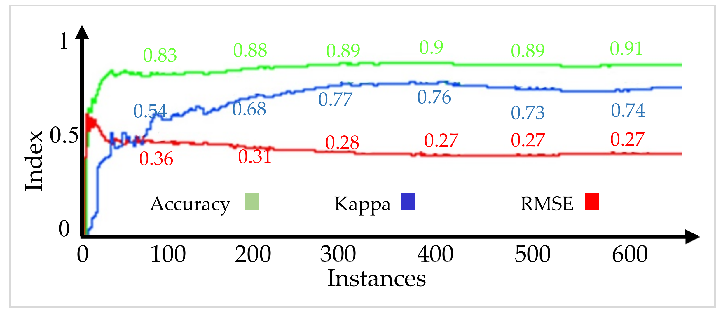
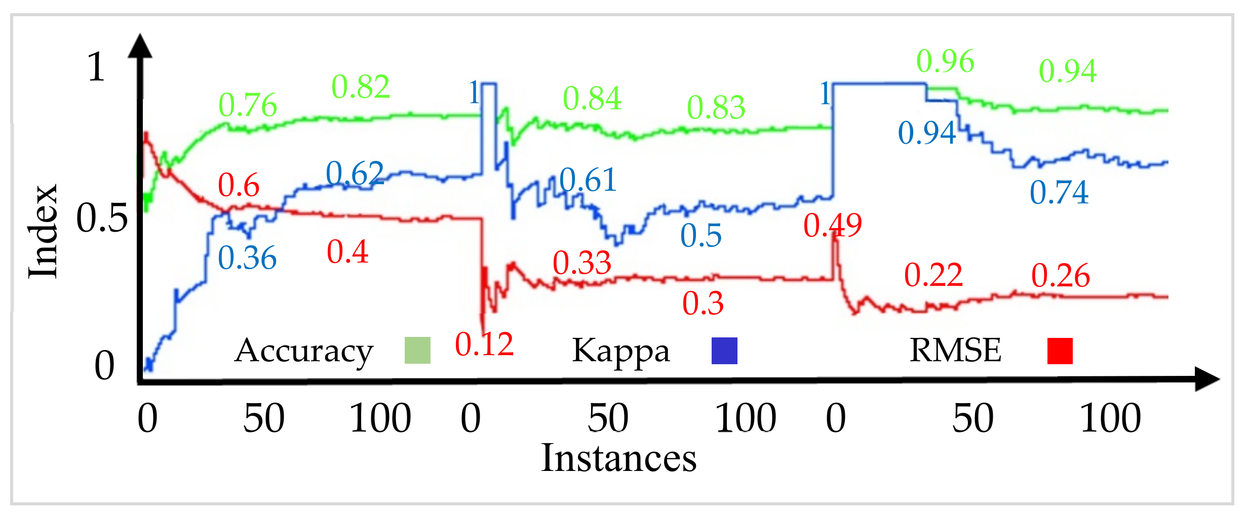
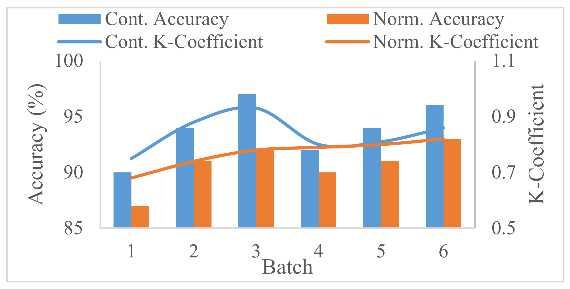
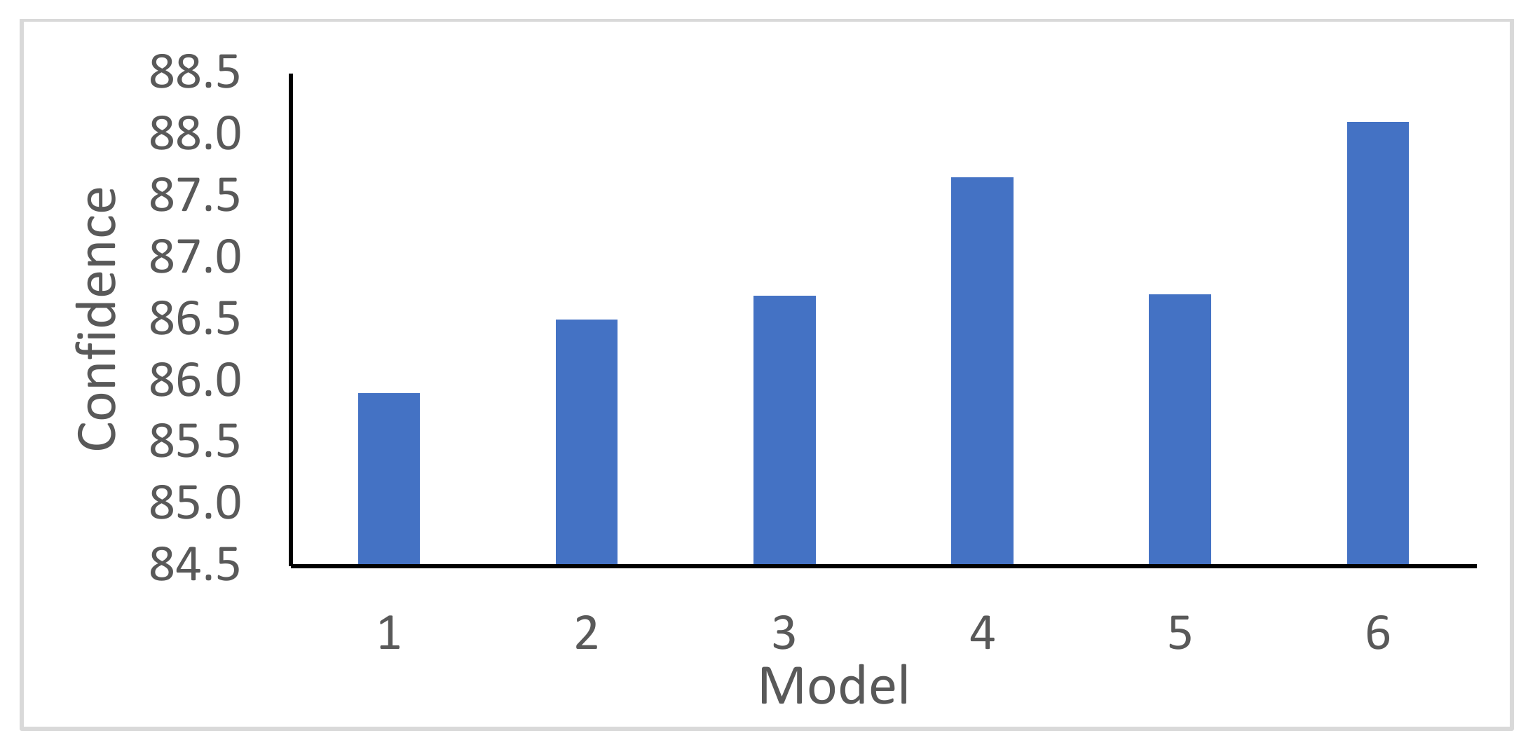
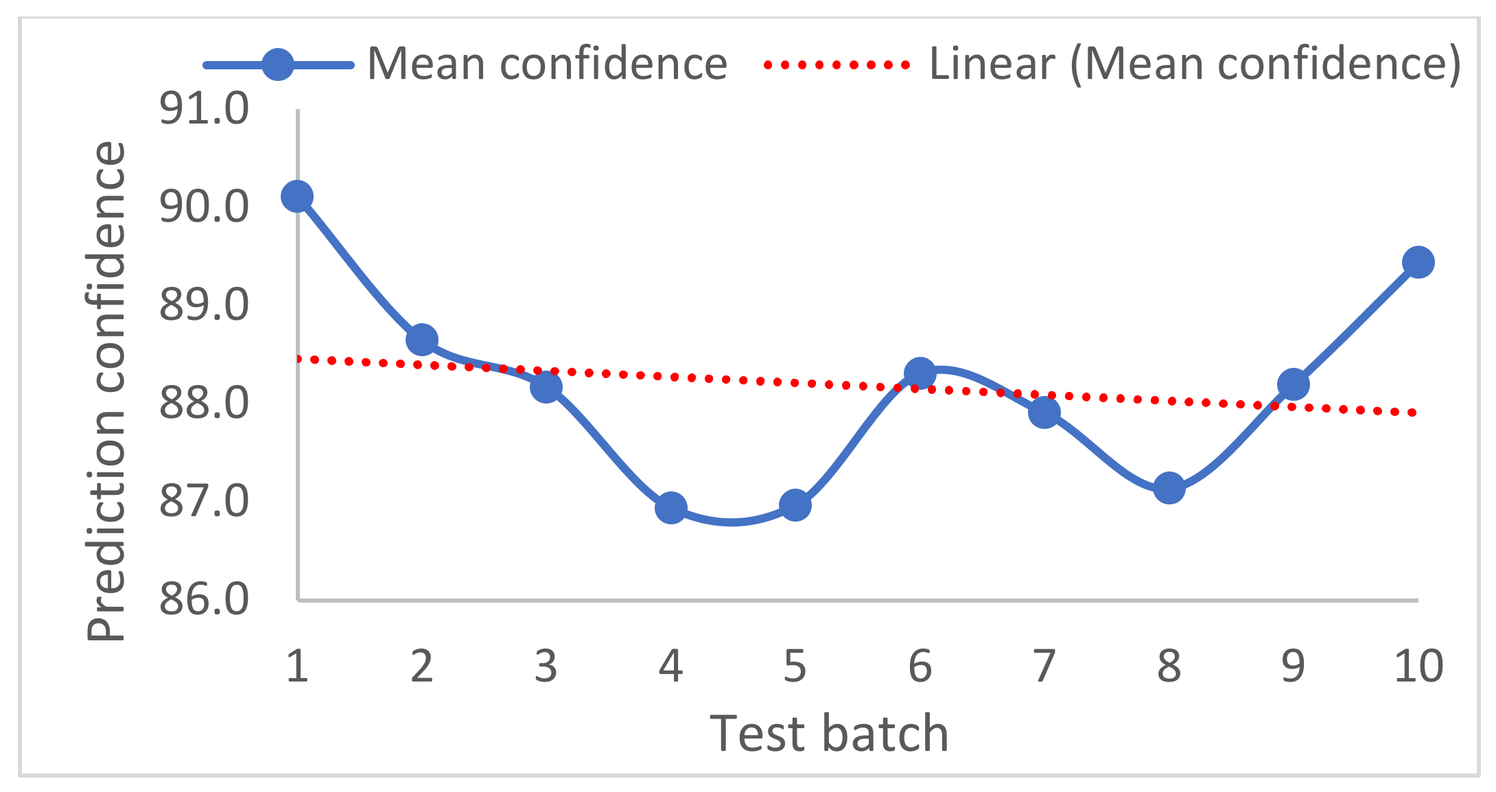
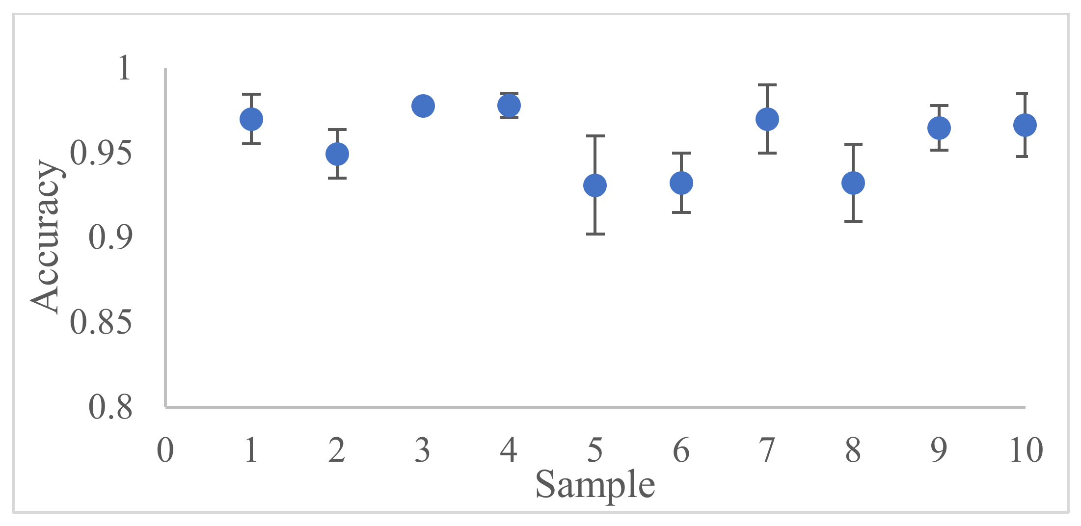
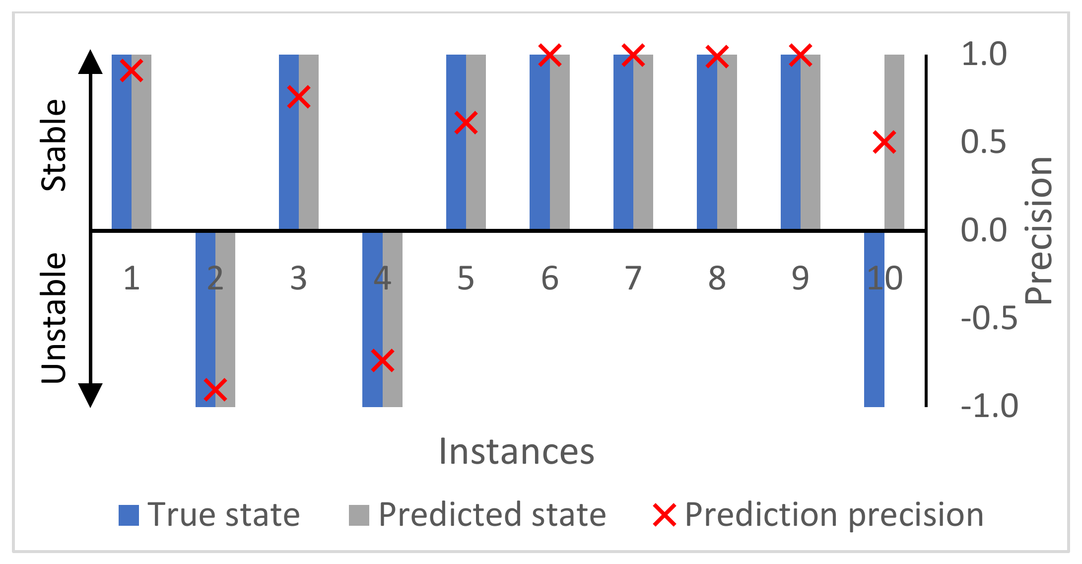
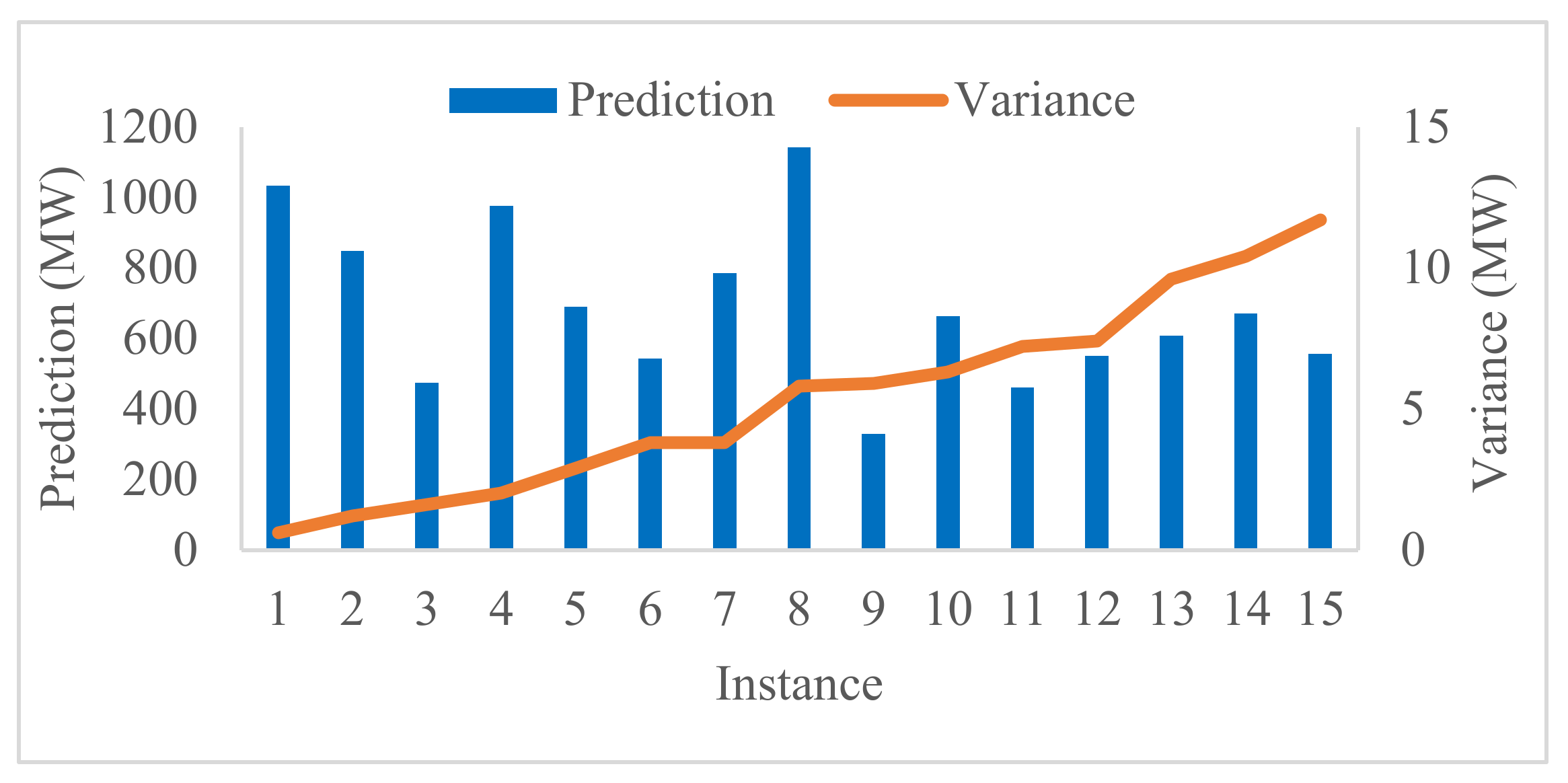
The security prediction models are obtained at the end of each batch training. The mean accuracy and standard deviation of 0.94 and 0.025, respectively, were obtained from six dataset batches of 100 instances per batch. A 90% accurate prediction of the security state of a testing dataset with 10 instances was obtained when compared to the true security state. The obtained AGRP model for security control was able to predict the load shed values within 50 MW variance for 30 test instances. A 100% secure state was achieved using the proposed optimal load shedding node identification. In conclusion, the proposed models can predict and control the security state of the emerging power grid under the described varying grid attributes.

Future research of this paper will focus on considering parallel computation techniques to improve the efficiency of the proposed online security prediction model, especially for very large power systems. It is also important to see how the Gaussian regression process model can be optimized to avoid unnecessary interruption of supply through appropriate hyperparameter selection. Although this paper has presented and discussed the possibility of implementing the proposed technique in a real power system, the deployment of the proposed model as an executable software for system operator utilization after being evaluated for robustness and scalability is a good consideration for future research. Lastly, considering that synthetic inertia is a tradable but costly commodity, the estimation of the optimal amount of synthetic inertia needed to ensure the stability of every unstable grid operation instance is also a significant and relevant future research area.

References

1. Arcia-Garibaldi, G.; Cruz-Romero, P.; Gómez-Expósito, A. Future power transmission: Visions, technologies and challenges. Renew. Sustain. Energy Rev. 2018, 94, 285–301. [Google Scholar] [CrossRef]
2. El-Hawary, M.E. The Smart Grid—State-of-the-art and Future Trends. Electr. Power Components Syst. 2014, 42, 239–250. [Google Scholar] [CrossRef]
3. Dranka, G.G.; Ferreira, P. Towards a smart grid power system in Brazil: Challenges and opportunities. Energy Policy 2020, 136, 111033. [Google Scholar] [CrossRef]
4. Hussain, S.M.S.; Nadeem, F.; Aftab, M.A.; Ali, I.; Ustun, T.S. The Emerging Energy Internet: Architecture, Benefits, Challenges, and Future Prospects. Electronics 2019, 8, 1037. [Google Scholar] [CrossRef] [Green Version]
5. Shakerighadi, B.; Peyghami, S.; Ebrahimzadeh, E.; Blaabjerg, F.; Back, C.L. A New Guideline for Security Assessment of Power Systems with a High Penetration of Wind Turbines. Appl. Sci. 2020, 10, 3190. [Google Scholar] [CrossRef]
6. Sridhar, S.; Hahn, A.; Govindarasu, M. Cyber–Physical System Security for the Electric Power Grid. Proc. IEEE 2012, 100, 210–224. [Google Scholar] [CrossRef]
7. Zhukov, A.; Tomin, N.; Kurbatsky, V.; Sidorov, D.; Panasetsky, D.; Foley, A. Ensemble methods of classification for power systems security assessment. Appl. Comput. Inform. 2019, 15, 45–53. [Google Scholar] [CrossRef] [Green Version]
8. Rezkalla, M.; Pertl, M.; Marinelli, M. Electric power system inertia: Requirements, challenges and solutions. Electr. Eng. 2018, 100, 2677–2693. [Google Scholar] [CrossRef] [Green Version]
9. Agarwal, U.; Jain, N. Distributed Energy Resources and Supportive Methodologies for their Optimal Planning under Modern Distribution Network: A Review. Technol. Econ. Smart Grids Sustain. Energy 2019, 4, 3. [Google Scholar] [CrossRef] [Green Version]
10. Vieira, S.; Pinaya, W.H.L.; Mechelli, A. Main concepts in machine learning. In Machine Learning; Elsevier BV: Amsterdam, The Netherlands, 2020; pp. 21–44. [Google Scholar]
11. Cai, W.; Zhang, M.; Zhang, Y. Batch Mode Active Learning for Regression with Expected Model Change. IEEE Trans. Neural Netw. Learn. Syst. 2017, 28, 1668–1681. [Google Scholar] [CrossRef]
12. Yang, Q.; Gu, Y.; Wu, D. Survey of incremental learning. In Proceedings of the 2019 Chinese Control And Decision Conference (CCDC), Nanchang, China, 3–5 June 2019. [Google Scholar]
13. Sharifzadeh, M.; Sikinioti-Lock, A.; Shah, N. Machine-learning methods for integrated renewable power generation: A comparative study of artificial neural networks, support vector regression, and Gaussian Process Regression. Renew. Sustain. Energy Rev. 2019, 108, 513–538. [Google Scholar] [CrossRef]
14. Jafarzadeh, S.; Genc, V.M.I. Real-time transient stability prediction of power systems based on the energy of signals ob-tained from PMUs. Electr. Power Syst. Res. 2021, 192, 107005. [Google Scholar] [CrossRef]
15. Yang, H.; Zhang, W.; Chen, J.; Wang, L. PMU-based voltage stability prediction using least square support vector machine with online learning. Electr. Power Syst. Res. 2018, 160, 234–242. [Google Scholar] [CrossRef]
16. Wang, G.; Zhang, Z.; Bian, Z.; Xu, Z. A short-term voltage stability online prediction method based on graph convolutional networks and long short-term memory networks. Int. J. Electr. Power Energy Syst. 2021, 127, 106647. [Google Scholar] [CrossRef]
17. Li, H.; Li, C.; Liu, Y. Maximum frequency deviation assessment with clustering based on metric learning. Int. J. Electr. Power Energy Syst. 2020, 120, 105980. [Google Scholar] [CrossRef]
18. Villa-Acevedo, W.M.; López-Lezama, J.M.; Colomé, D.G. Voltage Stability Margin Index Estimation Using a Hybrid Ker-nel Extreme Learning Machine Approach. Energies 2020, 13, 857. [Google Scholar] [CrossRef] [Green Version]
19. Mosavi, A.B.; Amiri, A.; Hosseini, S.H. A Learning Framework for Size and Type Independent Transient Stability Prediction of Power System Using Twin Convolutional Support Vector Machine. IEEE Access 2018, 6, 69937–69947. [Google Scholar] [CrossRef]
20. Tomin, N.; Kurbatsky, V.G.; Sidorov, D.; Zhukov, A. Machine Learning Techniques for Power System Security Assessment*. IFAC-PapersOnLine 2016, 49, 445–450. [Google Scholar] [CrossRef]
21. Huang, J.; Rimorov, D.; Moeini, A.; Kamwa, I.; Darvishi, A.; Fardanesh, B.; Babaei, S. Interconnection-level primary frequency control by MBPSS with wind generation and evaluation of eco-nomic impacts. Int. J. Electr. Power Energy Syst. 2020, 119, 1–10. [Google Scholar] [CrossRef]
22. Dreidy, M.; Mokhlis, H.; Mekhilef, S. Inertia response and frequency control techniques for renewable energy sources: A review. Renew. Sustain. Energy Rev. 2017, 69, 144–155. [Google Scholar] [CrossRef]
23. Dai, Y.; Xu, Y.; Dong, Z.; Wong, K.; Zhuang, L. Real-time prediction of event-driven load shedding for frequency stability enhancement of power systems. IET Gener. Transm. Distrib. 2012, 6, 914–921. [Google Scholar] [CrossRef]
24. Mo, N.-L.; Guan, Z.-H.; Zhang, D.-X.; Cheng, X.-M.; Liu, Z.-W.; Li, T. Data-driven based optimal distributed frequency control for islanded AC microgrids. Int. J. Electr. Power Energy Syst. 2020, 119, 105904. [Google Scholar] [CrossRef]
25. Liu, C.; Yang, R.J.; Yu, X.; Sun, C.; Wong, P.S.; Zhao, H. Virtual power plants for a sustainable urban future. Sustain. Cities Soc. 2021, 65, 102640. [Google Scholar] [CrossRef]
26. Zhong, W.; Murad, M.A.A.; Liu, M.; Milano, F. Impact of Virtual Power Plants on Power System Short-Term Transient Response. Electr. Power Syst. Res. 2020, 189, 106609. [Google Scholar] [CrossRef]
27. Bolzoni, A.; Perini, R. Feedback Couplings Evaluation on Synthetic Inertia Provision for Grid Frequency Support. IEEE Trans. Energy Convers. 2021, 36, 863–873. [Google Scholar] [CrossRef]
28. Guggilam, S.S.; Zhao, C.; Dall’Anese, E.; Chen, Y.C.; Dhople, S.V. Optimizing DER Participation in Inertial and Primary-Frequency Response. IEEE Trans. Power Syst. 2018, 33, 5194–5205. [Google Scholar] [CrossRef]
29. Singh, K.; Zaheeruddin. Enhancement of frequency regulation in tidal turbine power plant using virtual inertia from ca-pacitive energy storage system. J. Energy Storage 2021, 35. [Google Scholar] [CrossRef]
30. Feldmann, D.; Oliveira, R.V.d. Operational and control approach for PV power plants to provide inertial response and primary frequency control support to power system black-start. Int. J. Electr. Power Energy Syst. 2021, 127, 106645. [Google Scholar] [CrossRef]
31. Delavari, A.; Kamwa, I. Demand-Side Contribution to Power System Frequency Regulation: A Critical Review on De-centralized Strategies. Int. J. Emerg. Electr. Power Syst. 2017, 18. [Google Scholar] [CrossRef]
32. Kasis, A.; Devane, E.; Lestas, L. Primary frequency regulation in power networks with ancillary service from load-side par-ticipation. In International Federation of Automatic Control; Elsevier: London, UK, 2017. [Google Scholar]
33. Walger, Q.; Zuo, Y.; Derviškadić, A.; Frigo, G.; Paolone, M. OPF-based under frequency load shedding predicting the dynamic frequency trajectory. Electr. Power Syst. Res. 2020, 189, 106748. [Google Scholar] [CrossRef]
34. Sarwar, S.; Mokhlis, H.; Othman, M.; Shareef, H.; Wang, L.; Mansor, N.N.; Khairuddin, A.S.M.; Mohamad, H. Application of polynomial regression and MILP for under-frequency load shedding scheme in islanded distribution system. Alex. Eng. J. 2022, 61, 659–674. [Google Scholar] [CrossRef]
35. Alhelou, H.H.; Golshan, M.E.H.; Hatziargyriou, N.D. Deterministic Dynamic State Estimation-Based Optimal LFC for Interconnected Power Systems Using Unknown Input Observer. IEEE Trans. Smart Grid 2020, 11, 1582–1592. [Google Scholar] [CrossRef]
36. Silva, S.S., Jr.; Assis, T.M.L. Adaptive underfrequency load shedding in systems with renewable energy sources and storage capability. Electr. Power Syst. Res. 2020, 189, 106747. [Google Scholar] [CrossRef]
37. Ketabi, A.; Fini, M.H. Adaptive underfrequency load shedding using particle swarm optimization algorithm. J. Appl. Res. Technol. 2017, 15, 54–60. [Google Scholar] [CrossRef]
38. Sapari, N.; Mokhlis, H.; Laghari, J.A.; Bakar, A.; Dahalan, M. Application of load shedding schemes for distribution network connected with distributed generation: A review. Renew. Sustain. Energy Rev. 2018, 82, 858–867. [Google Scholar] [CrossRef]
39. Jallad, J.; Mekhilef, S.; Mokhlis, H.; Laghari, J.; Badran, O. Application of Hybrid Meta-Heuristic Techniques for Optimal Load Shedding Planning and Operation in an Islanded Distribution Network Integrated with Distributed Generation. Energies 2018, 11, 1134. [Google Scholar] [CrossRef] [Green Version]
40. Marchgraber, J.; Alács, C.; Guo, Y.; Gawlik, W.; Anta, A.; Stimmer, A.; Lenz, M.; Froschauer, M.; Leonhardt, M. Comparison of Control Strategies to Realize Synthetic Inertia in Converters. Energies 2020, 13, 3491. [Google Scholar] [CrossRef]
41. Lv, J.; Pawlak, M.; Annakkage, U.D. Prediction of the Transient Stability Boundary Based on Nonparametric Additive Modeling. IEEE Trans. Power Syst. 2017, 32, 4362–4369. [Google Scholar] [CrossRef]
42. Dhandhia, A.; Pandya, V.; Bhatt, P. Multi-class support vector machines for static security assessment of power system. Ain Shams Eng. J. 2020, 11, 57–65. [Google Scholar] [CrossRef]
43. Oliveira, W.D.; Vieira, J.P.; Bezerra, U.H.; Martins, D.A.; Rodrigues, B.D.G. Power system security assessment for multiple contingencies using multiway decision tree. Electr. Power Syst. Res. 2017, 148, 264–272. [Google Scholar] [CrossRef]
44. Li, Y.H.; Li, Y.; Sun, Y. Online Static Security Assessment of Power Systems Based on Lasso Algorithm. Appl. Sci. 2018, 8, 1442. [Google Scholar] [CrossRef] [Green Version]
45. Zhu, L.; Hill, D.J.; Lu, C. Hierarchical Deep Learning Machine for Power System Online Transient Stability Prediction. IEEE Trans. Power Syst. 2020, 35, 2399–2411. [Google Scholar] [CrossRef]
46. Su, L.; Qin, X.; Zhang, S.; Zhang, Y.; Jiang, Y.; Han, Y. Fast frequency response of inverter-based resources and its impact on system frequency characteristics. Glob. Energy Interconnect. 2020, 3, 475–485. [Google Scholar] [CrossRef]
47. Yu, Y.; Liu, Y.; Qin, C.; Yang, T. Theory and Method of Power System Integrated Security Region Irrelevant to Operation States: An Introduc-tion. Engineering 2020, 6, 754–777. [Google Scholar] [CrossRef]
48. Photovoltaics, D.G.; Storage, E. IEEE Standard Conformance Test Procedures for Equipment Interconnecting Distributed Energy Resources with Electric Power Systems and Associated Interfaces; IEEE Standard 1547.1-2020; IEEE: Piscataway, NJ, USA, 2020; pp. 1–282. [Google Scholar] [CrossRef]
49. Muzaffer, I.; Mufti, M.U.D. Modeling of a multi-machine system aided with power system stabilizers and shunt compensator for transient stability enhancement. In Proceedings of the 2017 International Conference on Energy, Communication, Data Analytics and Soft Computing (ICECDS), Chennai, India, 1–2 August 2021; IEEE: Manhattan, NY, USA, 2017. [Google Scholar]
50. Hoi, S.C.H.; Sahoo, D.; Lu, J.; Zhao, P. Online learning: A comprehensive survey. arXiv 2018, arXiv:1802.02871. [Google Scholar]
51. Luo, Y.; Yin, L.; Bai, W.; Mao, K. An Appraisal of Incremental Learning Methods. Entropy 2020, 22, 1190. [Google Scholar] [CrossRef] [PubMed]
52. Zhong, J.; Liu, Z.; Zeng, Y.; Cui, L.; Ji, Z. A Survey on Incremental Learning. 2017. Available online: https://webofproceedings.org/proceedings_series/ECS/CAPE%202017/CAPE_1113034.pdf (accessed on 25 September 2021).
53. Ren, S.; Lian, Y.; Zou, X. Incremental Naïve Bayesian Learning Algorithm based on Classification Contribution Degree. J. Comput. 2014, 9, 1967–1974. [Google Scholar] [CrossRef]
54. Cervantes, A.; Gagné, C.; Isasi, P.; Parizeau, M. Evaluating and Characterizing Incremental Learning from Non-Stationary Data. arXiv 2018, arXiv:1806.06610. [Google Scholar]
55. Chapaneri, S.; Lopes, R.; Jayaswal, D. Evaluation of Music Features for PUK Kernel Based Genre Classification. Procedia Comput. Sci. 2015, 45, 186–196. [Google Scholar] [CrossRef] [Green Version]
56. Vo, G.; Pati, D. Sparse Additive Gaussian Process with Soft Interactions. Open J. Stat. 2017, 7, 567–588. [Google Scholar] [CrossRef] [Green Version]
Figure 1. Emerging power grid with RES-DG units.
Energies 14 06639 g001
Figure 2. Frequency response under varying inertia.
Energies 14 06639 g002
Figure 3. System security region modelling.
Energies 14 06639 g003
Figure 4. Online system security modelling.
Energies 14 06639 g004
Figure 5. Proposed security control flowchart.
Energies 14 06639 g005
Figure 6. Incremental Naïve Bayes learning model.
Energies 14 06639 g006
Figure 7. Knowledge flow layout for proposed security state prediction.
Energies 14 06639 g007
Figure 8. Structure of the modern integrated power grid.
Energies 14 06639 g008
Figure 9. One-line diagram of the IEEE 39-bus system.
Energies 14 06639 g009
Figure 10. Security scenarios with RES-DG dispatch.
Energies 14 06639 g010
Figure 11. Security scenarios with load level.
Energies 14 06639 g011
Figure 12. Stability state inertia distribution.
Energies 14 06639 g012
Figure 13. Average inertia constant for RES-DG output.
Energies 14 06639 g013
Figure 14. Performance in normal training mode.
Energies 14 06639 g014
Figure 15. Performance in continual training mode.
Energies 14 06639 g015
Figure 16. Model batch performance indices.
Energies 14 06639 g016
Figure 17. Incremental model prediction confidence.
Energies 14 06639 g017
Figure 18. Mean prediction confidence.
Energies 14 06639 g018
Figure 19. Model mean accuracy.
Energies 14 06639 g019
Figure 20. True security and predicted security.
Energies 14 06639 g020
Figure 21. Load shedding distribution.
Energies 14 06639 g021
Figure 22. Load shedding density considering system inertia.
Energies 14 06639 g022
Figure 23. Load shedding density considering RES-DG output.
Energies 14 06639 g023
Figure 24. True load shed values vs. predicted load shed values.
Energies 14 06639 g024
Figure 25. Optimal node selection indices.
Energies 14 06639 g025