Article

A Sensitivity Matrix Approach Using Two-Stage Optimization for Voltage Regulation of LV Networks with High PV Penetration

by
A.S. Jameel Hassan
1,†,
Umar Marikkar
1,†,
G.W. Kasun Prabhath
1,
Aranee Balachandran
1,
W.G. Chaminda Bandara
1,
Parakrama B. Ekanayake
1,
Roshan I. Godaliyadda
1 and
Janaka B. Ekanayake
1,2,*
1
Department of Electrical and Electronic Engineering, University of Peradeniya, Peradeniya 20400, Sri Lanka
2
School of Engineering, Cardiff University, The Parade, Cardiff CF24 3AA, UK
*
Author to whom correspondence should be addressed.
These authors contributed equally to this work.
Energies 2021, 14(20), 6596; https://doi.org/10.3390/en14206596
Submission received: 23 August 2021 / Revised: 6 October 2021 / Accepted: 9 October 2021 / Published: 13 October 2021
(This article belongs to the Collection Feature Papers in Smart Grids and Microgrids)

Abstract

:
The occurrence of voltage violations is a major deterrent for absorbing more rooftop solar power into smart Low-Voltage Distribution Grids (LVDGs). Recent studies have focused on decentralized control methods to solve this problem due to the high computational time in performing load flows in centralized control techniques. To address this issue, a novel sensitivity matrix was developed to estimate the voltages of the network by replacing load flow simulations. In this paper, a Centralized Active, Reactive Power Management System (CARPMS) is proposed to optimally utilize the reactive power capability of smart Photovoltaic (PV) inverters with minimal active power curtailment to mitigate the voltage violation problem. The developed sensitivity matrix is able to reduce the time consumed by 55.1% compared to load flow simulations, enabling near-real-time control optimization. Given the large solution space of power systems, a novel two-stage optimization is proposed, where the solution space is narrowed down by a Feasible Region Search (FRS) step, followed by Particle Swarm Optimization (PSO). The failure of standalone PSO to converge to a feasible solution for 34% of the scenarios evaluated further validates the necessity of the two-stage optimization using FRS. The performance of the proposed methodology was analysed in comparison to the load flow method to demonstrate the accuracy and the capability of the optimization algorithm to mitigate voltage violations in near-real time. The deviations of the mean voltages of the proposed methodology from the load flow method were: 6.5 × 10 3 p.u for reactive power control using Q-injection, 1.02 × 10 2 p.u for reactive power control using Q-absorption, and 0 p.u for active power curtailment case.

Graphical Abstract

1. Introduction

Over the years, the integration of renewable Distributed Energy Resources (DERs) to Low-Voltage Distribution Grids (LVDGs) has gained high prominence due to technological advancements, increased demand in sustainable energy resources and the advent of decarbonisation programs by many countries [1,2,3]. In light of the increase in DERs, Photovoltaic (PV) generation systems are shown to be the most effective DER prospect for LVDGs [4]. However, since the conventional LVDG was designed based on the assumption that power flow would be from the primary substation to the loads [5], high PV penetration gives rise to unforeseen problems [6]. The high penetration of rooftop PV in LVDGs can result in reverse power flows [7] and an increase in the neutral current, leading to distribution and transformer losses due to overheating of the conductor [5,8,9,10,11]. A major problem of reverse power flow is the occurrence of upper limit voltage violations, where the node voltage at specific points of LVDGs is greater than the specified limit [12]. Further, studies have revealed that voltage violations can occur at a penetration level as low as 2.5% due to the integration of rooftop PV panels at prosumers’ will [13]. If such voltage violations occur over sustained periods of time, it will cause severe damages to loads connected to LVDGs. These detrimental effects of voltage violations compel the utility providers to limit the usable PV capacity for LVDGs. Therefore, there exists a crucial need for an effective solution to encourage the future integration of PV to LVDGs by attempting to mitigate the quality-of-supply ramifications. How to mitigate the voltage violations in LVDGs is a long-standing question to which much time and study have been devoted.
Multiple methods have been proposed in the literature to overcome this problem of voltage violations in LVDGs. Feeder enhancement is one such method based on changing the feeder cable with a larger cable or changing the characteristics of the feeder, such as changing the values of multigrounded resistances [14]. While this improves the voltage limits while decreasing neutral current, the approach is highly expensive. Moreover, given the future consumption and PV penetration possibilities, this is not the most economical solution. A more viable solution is the use of On-Load Tap Changing (OLTC) transformers to change the tap positions to control the voltage levels [15,16,17,18]. Furthermore, since frequent tap changes can increase the stress on the transformer, hence reducing its lifespan, a novel optimization algorithm was proposed for resource sharing in [19] to reduce the tap changing operations. However, the drawback of the slow response speed in OLTC switching persists. In order to remedy this issue, fast response devices such as Battery Energy Storage Systems (BESSs) and STATCOMs can be installed [20,21,22,23,24]. A piecewise droop control using a BESS for rapid changes in voltage profiles was presented in [25]. More recently, a reinforcement-learning-based management technique for BESSs was introduced in [26].
A more promising control method is the use of Active Power Curtailment (APC) during high PV penetration [27,28,29,30]. Due to the higher impact on voltage profiles by nodes at the farther end of the feeder, most APC operations are performed on distant customers. Since this is not equitable, a fair prosumer-based APC approach was proposed in [31]. A novel approach incorporating the Self-Consumption Ratio (SCR) of the customer to determine the allowable PV injection was developed in [32]. Despite the effectiveness, the spilling of solar power is not an economically attractive solution. Moreover, it is a waste and also detrimental to the whole purpose of renewable energy usage, which is to improve the energy mix such that the renewables receive a larger chunk. A more comprehensive solution to this problem is to utilize the capability of the PV inverters to the fullest to supply reactive power in order to mitigate voltage violations. Whilst this is a cost-effective method requiring no additional installations, mitigating voltage violations in the three-phase unbalanced system using only Reactive Power Control (RPC) is a challenging problem [33,34]. Due to the large R/X ratios of distribution networks, the effect of reactive power control is limited. Therefore, to completely remove the violations in the upper limit, APC is required.
Recent studies have vastly explored the APC and RPC mechanisms to minimize voltage violations. These studies can be categorized into two: local/decentralized control and centralized control methods. Control actions of decentralized control methods rely completely on local measurements [35,36,37,38,39]. A combined approach of RPC and APC as a droop control mechanism to mitigate the voltage violations was proposed in [34]. A Volt-VAR Control (VVC) using two methods to determine the reactive power equation slope was given in [40]. It presented a method with the robust minimization of absolute voltage deviation and a closed-form solution inspired by chance constraints. In [41], a rule-based decentralized RPC was performed taking into account the most sensitive nodes in the network. An optimization technique was developed in [42] to coordinate the fast dispatch of PV inverters with OLTCs in a decentralized manner due to computational burden in centralized systems. Meanwhile, a two-level control algorithm incorporating OLTCs and BESSs with decentralized RPC was proposed in [43]. Multiple works in the literature have also developed control mechanisms based on droop control [44,45]. Nevertheless, the lack of information about the entire network status in decentralized control prevents the optimal use of reactive power capacity in controlling the voltage violations. Therefore, an uncoordinated management of PV inverters could result in violations shifting from one end of the feeder to another, or even an overkill of reactive power usage [46]. This gap in the lack of coordination among PV inverters has led to the use of optimization techniques based on a centralized system to address this [47]. Moreover, the prevalence of decentralized control has primarily hinged on the computational time burden in centralized systems [48]. However, this constraint is overcome by replacing the time-consuming load flow calculations by the introduced sensitivity matrix approximation in this paper.
However, provided that sufficient information about the network can be retained, centralized control is more efficient compared to decentralized control [46]. Such network state observability is achieved by means of solar predictions [49] and state estimation [50], enabling a control at the tertiary level of the control architecture, as shown in Figure 1. To overcome the lack of information about the network, a global solution is attained by the centralized control method, which determines the power injections/absorptions/curtailment by means of an Optimal Power Flow (OPF) problem [51]. In [52], a comprehensive PV control strategy was proposed to improve the operational performance of significantly unbalanced a three-phase four-wire LVDG with high residential PV penetration, by converting a multi-objective OPF problem into a single-objective OPF problem. A control algorithm was introduced for maintaining the average customer voltage profile obtained before introducing the PV into the circuit using the control of automatic devices, such as voltage regulation and switched capacitor banks along with PV inverter reactive power [53]. Here, the PV inverter control settings were determined by the circuit loading, time of day and PV location in the network. A combination of centralized and decentralized control strategies utilising OLTCs and Capacitor Banks (CBs) was also proposed in [47,54]. It further analysed the impact on the substation end and the effect of unbalance in phases in PV integration.
However, these methods suffer from a high computation time due to varying reasons such as the need to solve load flows within the optimization algorithm and the integration of VAR compensation equipment. Most of the referenced centralized methods related to power systems control use load flow analysis to calculate voltage variation [55,56,57]. Since these methods achieve accurate results at the expense of time, a voltage and PV power sensitivity approach is used to calculate the voltage variations [27,58,59,60,61]. The different sensitivity matrices used in the literature are discussed in Table 1.
In order to find the optimum solution to the centralized control method in mitigating voltage violations, many optimization techniques have been researched. Among these, SQP [52], Nonlinear Programming (NLP) [62,63], the Evolutionary Algorithm [64], Lagrangian multipliers [65], the Multi-Objective Evolutionary Algorithm (MOEA) [66] and Particle Swarm Optimization (PSO) [55,67] have been widely used. In order to act as a viable near-real-time system, the accuracy and the computational time of the algorithm play a key role. Given the vast solution space of LVDG networks, i.e., high complexity of the network due to the number of PV connections in the power system, the computational time for convergence grows dramatically. Therefore, optimization techniques need to be tailored to LVDG power systems such that the computational time is minimal whilst maintaining robustness in terms of convergence to the optimal solution.
In this paper, we propose a Centralized Active, Reactive Power Management System (CARPMS), which uses the combination of both RPC and APC to mitigate the voltage violations in LVDGs at the tertiary control level. A sensitivity matrix derivation for the voltage with respect to the PV power changes and a modified two-stage optimization process with a Feasible Region Search (FRS) and PSO, to find the optimal power settings, were developed. The incorporation of the sensitivity matrix vastly reduced the computational time as compared to traditional load-flow-based optimization in centralized control. In addition, the FRS step in the two-stage optimization process was able to greatly reduce the search space for the solution by narrowing the solution towards the optimum and decreasing the time, thereby enabling a real-time application of the proposed solution. The PSO algorithm was used as the second step to drive the solution to its best solution to prevent frequent violations in the network.
The proposed CARPMS was simulated on a network belonging to an existing housing complex named “Lotus Grove”, located in Colombo, Sri Lanka. The case study network was chosen from the same region of the authors whilst being similar to the IEEE European low-voltage test feeder [68,69] in network size and topology. Specifically, the following contributions were made in this paper:
  • A novel PV-power to voltage Sensitivity Matrix (SM) for LVDGs was developed using line parameters accounting for the voltage variations in the secondary side;
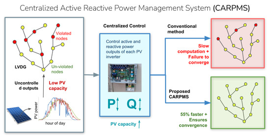
  • A Centralized Active, Reactive Power Management System (CARPMS) using this SM for voltage violations in LVDGs is proposed;
  • A modified two-stage optimization process is proposed, with the Feasible Region Search (FRS) as an efficient space reduction algorithm to decrease the computational time and ensure convergence of the PSO optimizer that follows it.

2. Methodology

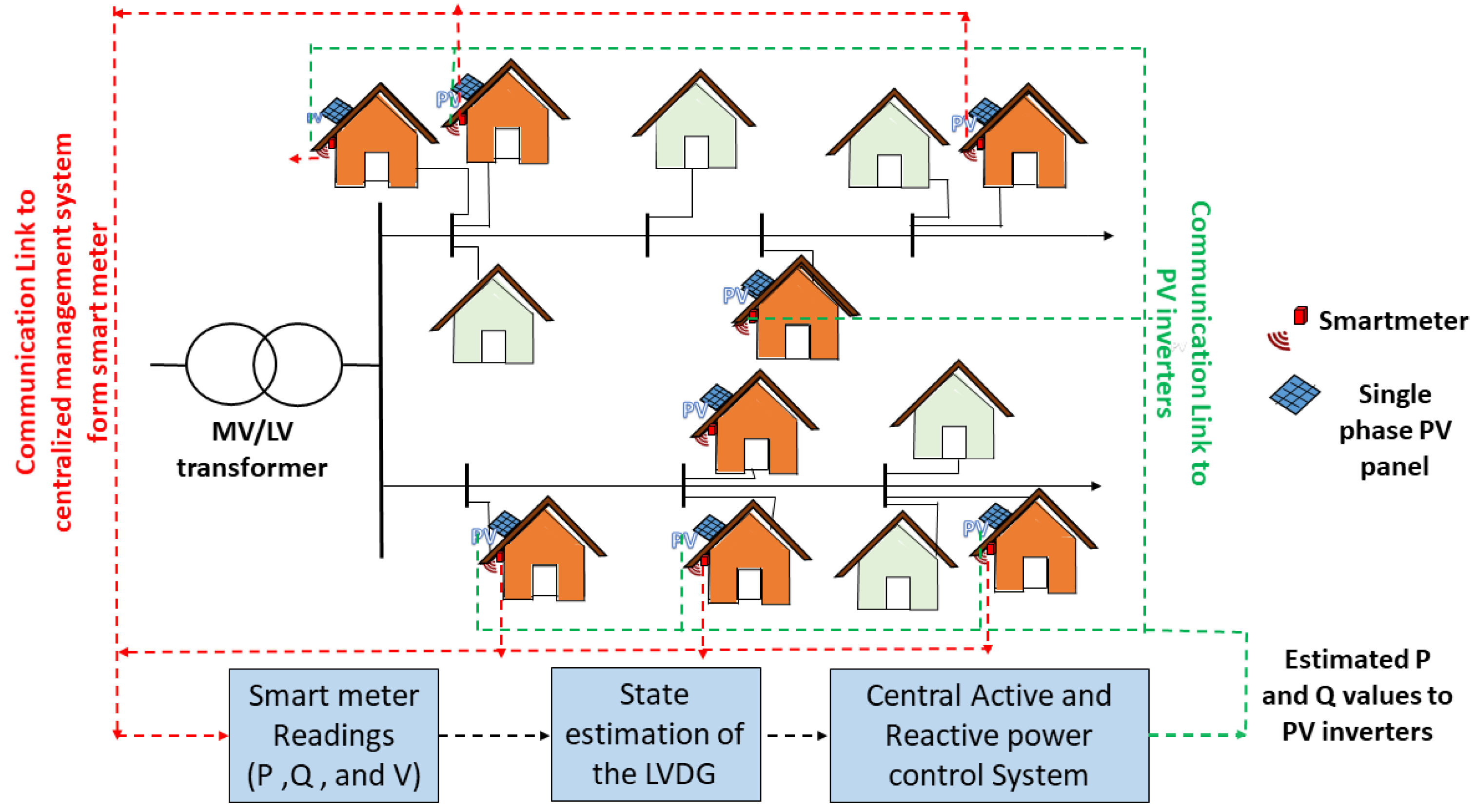
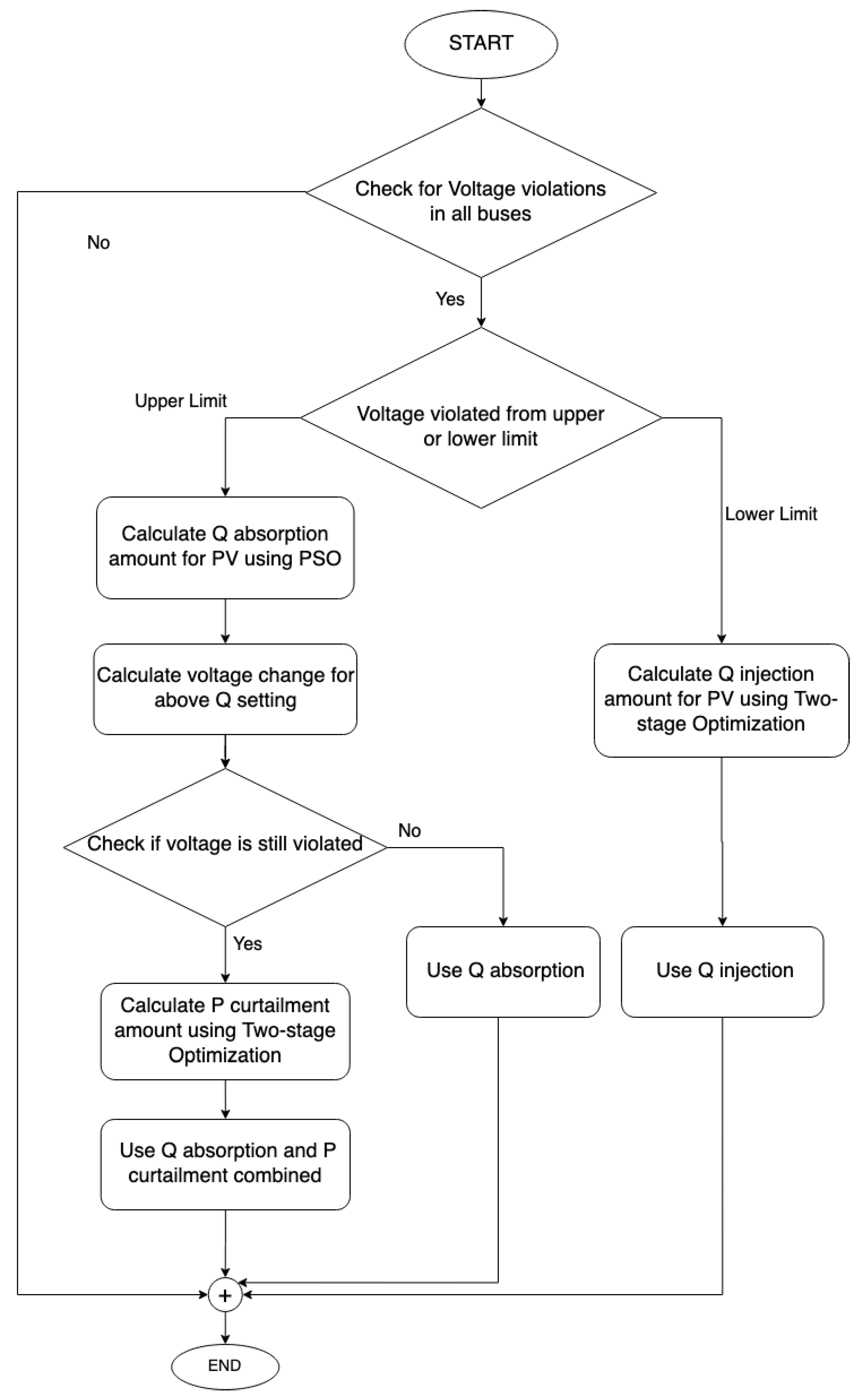
2.1. Centralized Active, Reactive Power Management System

In this section, the proposed CARPMS, which eliminates the voltage limit violations at each node, is described. Figure 2 shows the operating mechanism of the CARPMS. The CARPMS is equipped with smart meters at each PV panel in the network, ensuring the access to active, reactive power and voltage readings at each PV panel node. Due to delays incurred in communication and algorithm processing time [70], real-time data will not reach the CARPMS. Therefore, it acts as a real time management system with control actions relying on estimations of the network states predicted using historical data [50]. The proposed algorithm described in Section 4 is then used by the CARPMS to detect and correct any voltage violations in the nodes.
The proposed algorithm will encounter voltage violations of two types: upper limit and lower limit violations. Due to the low X/R ratio, the violations cannot be entirely removed by RPC alone. In this case, the algorithm utilizes an optimized combination of RPC and APC. A detailed flow of the algorithm steps is highlighted in Figure 3. The derivation of the SM used is given in Section 2.2, Section 2.3 and Section 2.4, and the two-stage optimization in the control algorithm is described in Section 3 and Section 4.

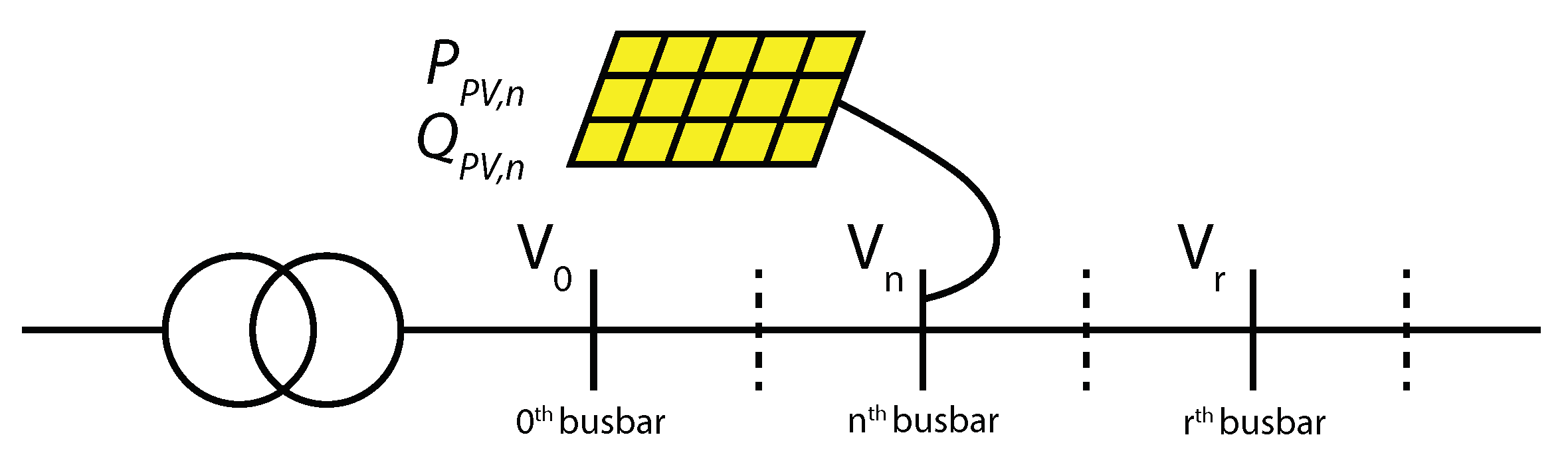
2.2. Voltage Sensitivity Derivation for the Distribution Line

The SM is derived for a network without sparse line connections. This assumption was made for the ease of proof, which can be easily extended for a network with sparse line connections if necessary.
Consider a phase of a distribution line shown in Figure 4. Due to the negligible effect of the longitudinal component, by neglecting the power losses, the voltage drop between any kth and ( k + 1 ) th node is given by,
| V k V k + 1 | P k R k + Q k X k | V k * |
where V k , V k + 1 are the complex voltages at the kth and ( k + 1 ) th nodes, respectively, R k is the resistance of the line, X k is the reactance of the line, P k is the active power flow through the line and Q k is the reactive power flow through the line.
The equation above expresses the difference in the magnitude of the voltage between two adjacent nodes. This equation was extended to calculate the voltages of all the nodes in the network. To generalize, a radial LVDG network with ( N + 1 ) number of nodes was considered. Considering the power flow from the LV transformer in the network as positive power flow and using (1), the voltage drop up to the rth node from the transformer end is given by,
| V 0 V r | = h = 0 r 1 P h R h + Q h X h | V h * |
where V 0 is the secondary voltage of the transformer for one of the three phases a, b or c, which is also the zeroth node of the network.
The power flow of the transmission line is a collective function of domestic loads, PV generations and power transmission losses. However, the power transmission losses are negligible compared to other variables. Thus, the power transmitted through the transmission line was derived as follows, which can be substituted in (2), yielding,
P h + j Q h = m = h + 1 N ( P L m P P V m ) + j ( Q L m Q P V m )
| V 0 V r | = h = 0 r 1 m = h + 1 N ( P L m P P V m ) R h + ( Q L m Q P V m ) X h | V h * |
The network parameters X h and R h given in (4) are constant, unique and attainable for every LVDG network. Whilst the load power and PV power generation parameters are not easily obtainable in real time, the estimation of these parameters is possible [71,72,73,74,75]. The derivation of the voltage of the rth node with respect to the reactive power of the PV system in the nth node was derived as,
V r Q P V n = V 0 Q P V n + h = 0 n 1 X h | V h * | f o r ( r n )
V r Q P V n = V 0 Q P V n + h = 0 r 1 X h | V h * | f o r ( r < n )
where V r Q P V n is the voltage sensitivity of the rth node with respect to the reactive power variation of the PV panel at the nth node and V 0 is the voltage of the node connected at the secondary side of the transformer. A schematic LVDG network showing the node notations is shown in Figure 4.
Similarly, the voltage sensitivity of nodes with respect to the active power of the PV system in the nth node can be derived.

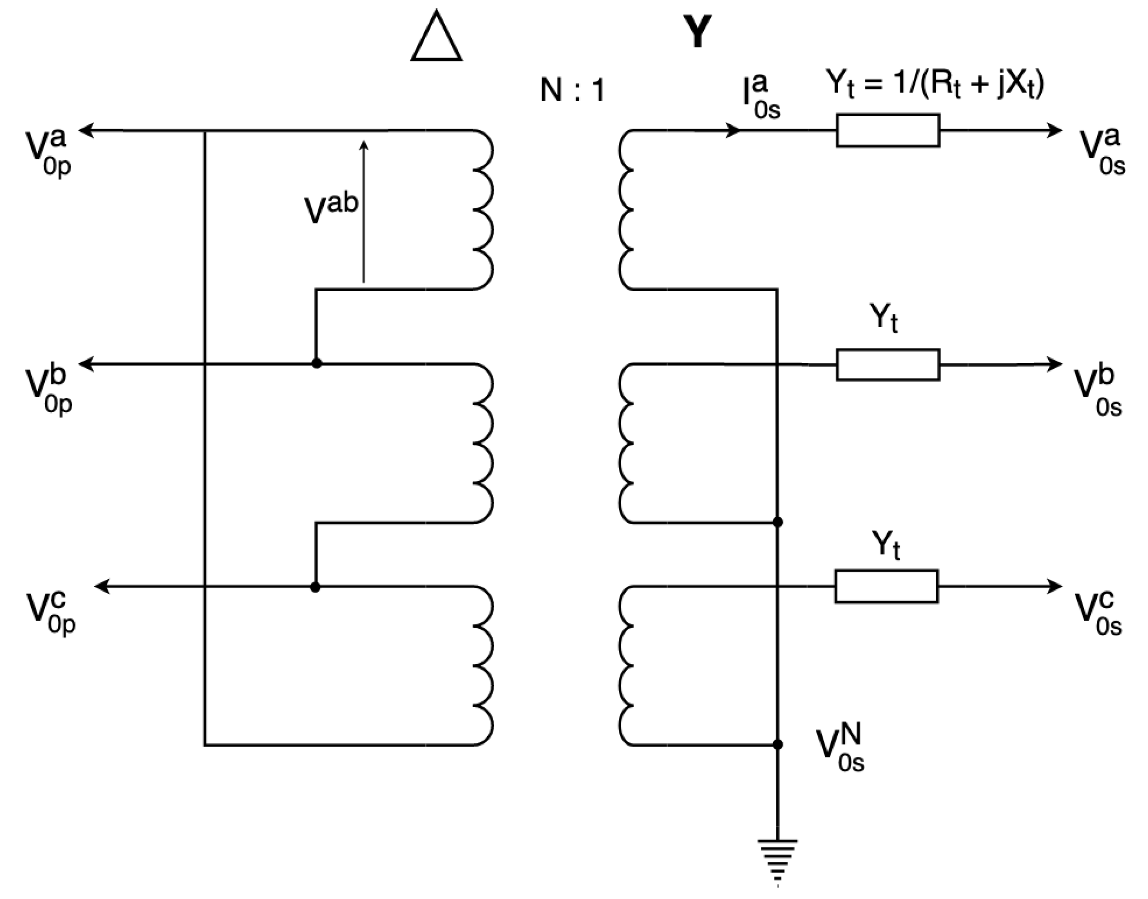
2.3. Voltage Sensitivity Derivation at the Transformer End

In order to calculate V 0 Q P V n and similarly V 0 P P V n , the LV transformer of the residential network was modelled as shown in Figure 5.
Considering the secondary side of the transformer, the expression for current and power flow in the secondary side was derived in terms of voltages and impedances using the transformer model matrix in [76]. The power flow in the secondary side of the transformer was obtained as,
P s a j Q s a = ( V 0 p a · Y 1 V 0 p b · Y 1 + V 0 s N · Y 2 ) | V 0 s a | δ k | V 0 s a | 2 · Y 2
where V 0 p a , V 0 p b and V 0 p c are the primary side voltages of the LV transformer, V 0 s a , V 0 s b and V 0 s c (generically denoted by V 0 in the previous section) are the secondary side voltages of the LV transformer and I 0 s a , I 0 s b and I 0 s c are the secondary side currents of the LV transformer of the a, b and c phases, respectively. Y 1 and Y 2 are the primary and secondary side impedances of the LV transformer, and N is the secondary to primary transformer turn ratio. Y 1 = Y t N , and Y 2 = Y t , V 0 s a = | V 0 s a | δ a .
In order to calculate the voltage sensitivity of the transformer end with respect to reactive power changes, the derivative of the imaginary component of (7) with respect to V 0 s a was obtained as,
Q s a | V 0 s a | = 2 | V 0 s a | · I m ( Y 2 ) I m ( ( V 0 p a · Y 1 V 0 p b · Y 1 + V 0 s N · Y 2 ) δ a )
Since the active and reactive power of loads can be assumed to be constant during a control sequence operation, using (3), the variation of reactive power for a given phase with respect to the transformer end voltage is only the variation of PV power in that phase.
Then, by obtaining the reciprocals, the variation of the transformer end voltage with respect to the PV reactive power connected to the given phase was computed using Equation (8).
| V 0 s a | Q P V a = | V 0 s a | Q s a
Similarly, using the real part of (7), the variation of the transformer end voltage with respect to the PV active power can be obtained.

2.4. Combined Sensitivity Matrix Model

The combined sensitivity model was derived based on the results from Section 2.2 and Section 2.3. Considering the number of PV panels in the system as M and the number of nodes in the system as N, using Equations (5), (6) and (9) and their analogous equations for active power, the combined SM model of the network with respect to the power generation of PV systems was derived as,
Δ V N × 1 = V Q P V V P P V N × 2 M Δ Q P V Δ P P V 2 M × 1 = h X h | V h * | h R h | V h * | N × 2 M Δ Q P V Δ P P V 2 M × 1 + Δ V 0 1 1 1 N × 1
where Δ V 0 N × 1 is the voltage change at the LV transformer end to be added to each node and Δ V N × 1 is the combined voltage variation at each node due to the PV power variations (at each iteration). The system was linearized assuming that the variation in the PV system power within the control sequence algorithm is considerably small.

3. Problem Formulation

The aim of this work was to determine an optimum setting to prevent voltage violations in LV networks. An RPC mechanism followed by APC is carried out if RPC alone is unable to rectify the voltage violations. Thus, two optimization functions defined in Section 3.1 and Section 3.2 were proposed to converge on the optimal operating point. The objective functions of the optimization algorithms intend to minimize the active and reactive power settings whilst satisfying the voltage limit constraints and the inverter constraints. The voltage limits pertain to the lower and upper limits of the acceptable voltages in LVDG networks, whereas the inverter constraints depend on the power ratings of the inverters.
The state of the PV inverter being varied by the algorithm depending on the three control methods Q-absorption, P-curtailment and Q-injection is depicted in Figure 6. The “X” mark shows an instance of an initial state of the inverter during the day. During RPC Q-absorption, the state moves vertically downwards to a given optimum point. If it reaches the inverter constraint/capability curve, this implies that Q-absorption cannot be performed under the given conditions. Then, P-curtailment is performed during which the state of the inverter moves along the capability curve, reducing the amount of active power injected to the network. It can also be noted that the maximum allowable value of Q-absorption, Q a b s , m a x , varies depending on the active power state of the inverter. The inverter state during night-time is marked “Y”. Here, RPC (Q injection) is carried out, and the inverter state moves upwards along the Q-axis (injecting reactive power to the network) till it reaches an optimal point or its full Q injection capacity: Q i n j , m a x .

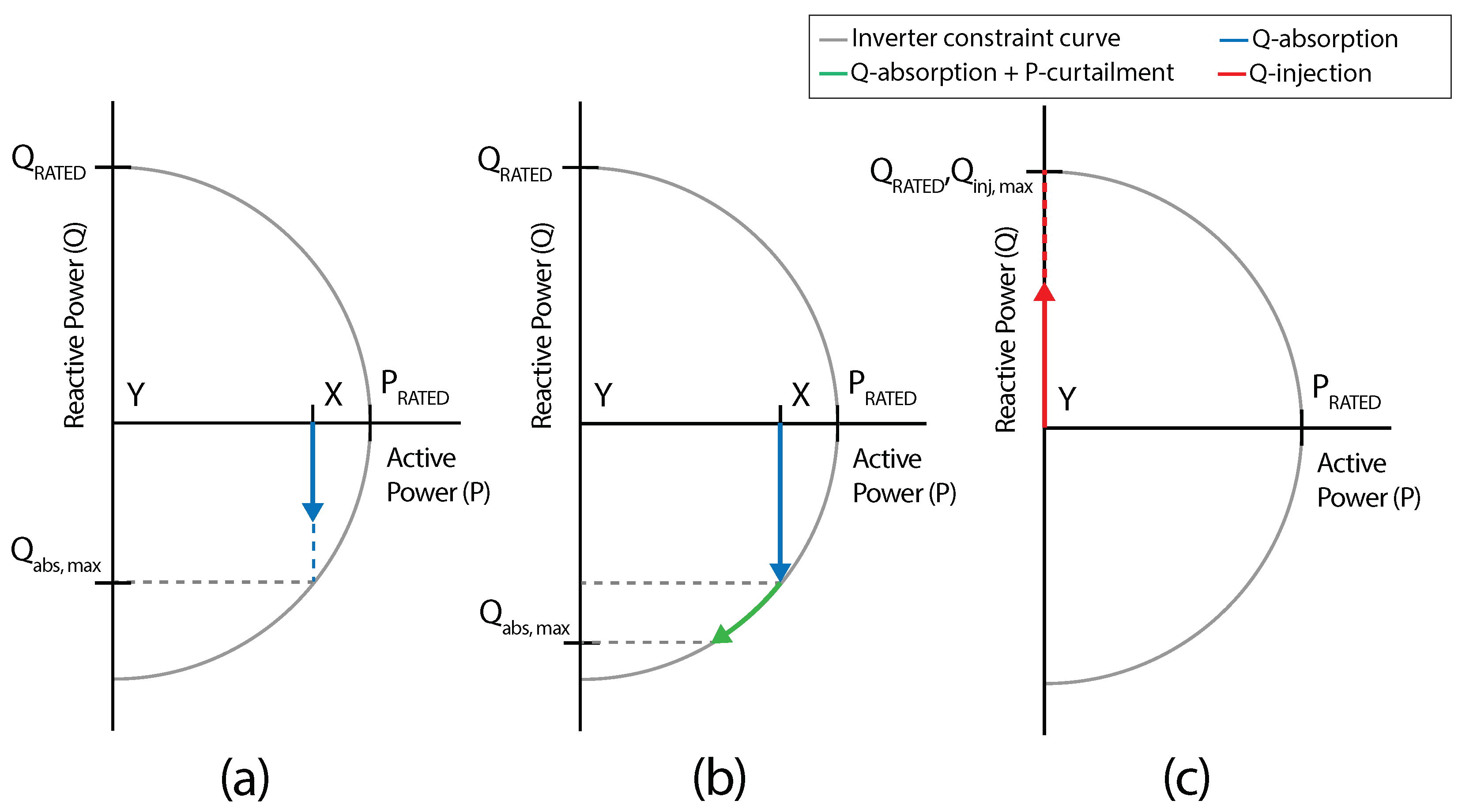
3.1. Optimization of Reactive Power Control

The objective function of the optimization of RPC is expressed as a function of the total deviation of node voltages from 1 p.u and the neutral voltage as given by,
J R P C = min Q i = 1 n c d V d , i + c n e u t V n e u t , i
where V d , i is the total deviation of voltages of node i from 1 p.u, V n e u t , i is the neutral voltage of node i and c d and c n e u t are scaling constants. V n e u t , i is calculated by the vector addition of the three-phase voltages of node i.
Subject to the constraints:
1.
The voltage of the node should be within the specified upper and lower limits given by,
V lower limit V nodes + Δ V V upper limit
where V lower limit and V upper limit are the accepted lower (0.95 p.u) and upper limit (1.05 p.u) voltages in LVDG systems, respectively, V nodes is the calculated voltage of the nodes using optimization variables and Δ V is the estimated voltage change due to changes in P and Q of the PV systems;
2.
The inverter constraints given below should be satisfied,
S P V i 2 P P V i 2 + Q P V i 2
The variables of the optimization problem were the reactive power setting at each node with a PV panel in the network, which can be expressed as O p t i m . V a r i a b l e ( O V ) Q = Q p v 1 , Q p v 2 , Q p v 3 , Q p v 4 , , Q p v m .
In order to formulate this optimization problem to minimize (11) whilst satisfying the above constraints, penalties were introduced to ensure that the optimal solution satisfies the constraint of voltage violations to the best case possible by penalising the cost function when constraints are violated. Hence, the optimization problem was reformulated as a minimisation of the penalized objective function J 1 given by (14).
J 1 = min Q c v i a l e N v i a l J R P C
where N v i a l is the sum of the number of violations in each phase and c v i a l is a scaling constant.

3.2. Optimization of Active Power Curtailment

The objective function of the optimization of APC included the amount of active power curtailed and is expressed as,
J A P C = min P i = 1 n Δ P P V i + c d V d , i + c n e u t V n e u t , i
where Δ P P V i is the amount of curtailed active power, V d , i is the total deviation of voltage of node i from 1 p.u, V n e u t is the neutral voltage of node i and c d and c n e u t are scaling constants.
Subject to the constraints:
1.
The voltage of the nodes should be within the specified upper and lower limits as in (12);
2.
The inverter constraint given below should be satisfied,
S P V i 2 = P P V i 2 + Q P V i 2
The variables of the optimization problem here were the active power setting at each node in the network, which can be expressed as O p t i m i z a t i o n v a r i a b l e ( O V ) P = [ P p v 1 , P p v 2 , P p v 3 , P p v 4 , , P p v m ] .
Similar to the RPC case, the optimization problem was reformulated by including the same penalties such that the penalty is applied when the constraint is violated. This ensures the optimal solution of the objective function satisfies all constraints.

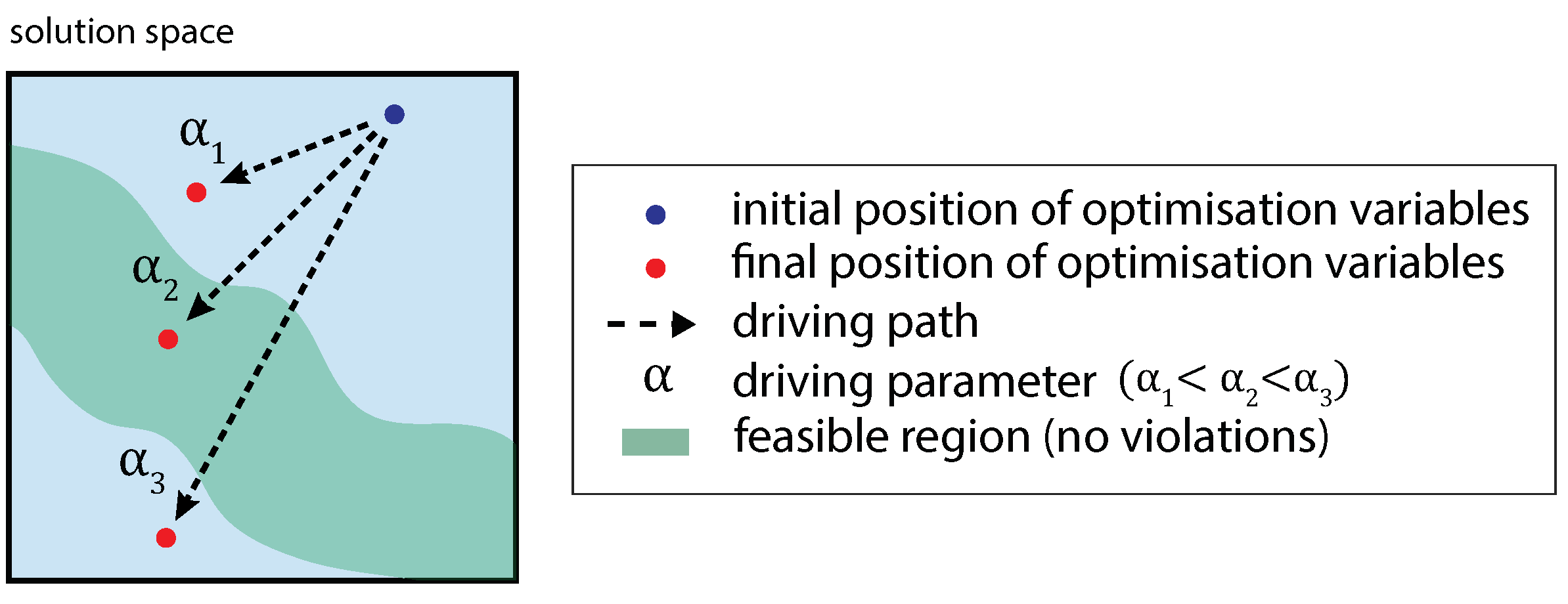
4. Two-Stage Optimization

This section outlines the proposed modified optimization algorithm consisting of two processes in sequence:
  • Feasible Region Search (FRS);
  • Particle Swarm Optimization (PSO).
The aim of FRS is to drive the elements in the Optimization Variable ( O V ) towards the feasible region, where upper or lower limit voltage violations are nonexistent. This is followed by a PSO algorithm, where these variables in the feasible region are then optimized according to a predefined cost function, to find the best possible solution.

4.1. Feasible Region Search

The number of elements in the O V increases with the number of PV panels connected to a given network, which results in a large search space. At the initial violated conditions, the existence of the O V far away from the feasible region and the high dimensionality of the search space may result in the poor performance of a standard PSO algorithm. This is because the first step of the PSO is an initialisation procedure (discussed in Section 4.2), being a random scattering of O V s in the neighbourhood of the current O V .
Through FRS, we determine a new initial point for the PSO by moving the present O V towards the feasible region. The driving function of the O V is given by,
O V [ i , j ] = O V [ 1 , j ] + α [ i ] Δ O V m a x [ j ]
for all j = 1 , 2 m ( total number of elements in O V [ i , : ] ) , where O V [ 1 , j ] is the initial value of the jth element in the O V , driven towards the feasible region by α [ i ] . Here, α [ i ] is the driving parameter, which is a monotonically increasing function from 0–1. Δ O V m a x [ j ] is the maximum possible change of O V [ : , j ] . This results in O V [ i , j ] , the calculated position of the jth element of the O V at the ith iteration.
In a PV integrated network, the vector O V [ i , : ] is the power settings of each inverter connected to the network at any given iteration i. Δ O V m a x [ j ] is the maximum Q-absorption, Q-injection or P-curtailment capacity of the jth inverter. This also determines the driving direction of the elements of O V , as the sign of Δ O V m a x [ j ] is dependent on the current nature of the voltage violation. In the instance of an upper limit violation, Δ O V m a x [ j ] will be negative, as the P and Q setting of the jth inverter, which correspond to the maximum P-curtailment and Q-absorption capacity, are negative. Δ O V m a x [ j ] will be positive for lower limit violations, as the inverter state travels in the direction of positive Q for Q-injection, as discussed in Section 3.
During each iteration, O V [ i , j ] is computed such that it moves closer to the feasible region. As the sign of Δ O V m a x [ j ] ensures the current O V [ i , : ] moves towards the feasible region, the driving parameter α serves to gradually increase the change in O V [ : , j ] . If this change happens to be very large, there exists a possibility of O V overshooting towards unwarranted solutions, as illustrated in Figure 7. For example, lower limit violations may occur if Q-absorption takes place at its maximum capacity to mitigate an upper limit violation. This problem is overcome by the use of α , which gradually increases with each iteration i, allowing FRS to terminate as soon as O V [ i , j ] reaches the feasible region.
For most instances, upon the termination of FRS, the system is devoid of any upper or lower limit violations. Although it is possible to complete the control process using only FRS, it does not fully optimize the network as it does not consider parameters relative to the cost function given by (14) and (15). Instead, it only accounts for the existence of violations in the system. Furthermore, FRS acts as a decoupled control algorithm, where the inverter power settings in the ith iteration are independent of each other, where each element in O V [ i , : ] is modified by the same value of α . However, in the case that the FRS is unable to drive the O V to the feasible region, it is ensured that the O V is as close as possible to the feasible region. In the case of FRS on an upper limit violation, if a lower limit violation emerges, the FRS is terminated when the total number of violations is minimum. Similarly, in the case of FRS on a lower limit violation, if an upper limit violation emerges, FRS is terminated when the total number of violations is again minimum. This establishes that the final O V from the FRS is as close to the feasible region and beyond adequate as an initialization for the PSO.
Although slower than FRS, the PSO algorithm performs as a collective control algorithm. This implies that the factor α at which Q-absorption, Q-injection or P-curtailment is performed relative to the capacity of the inverter will be optimized. For instance, in the absence of solar power, PSO will ensure more Q is injected to the network by inverters furthest from the secondary transformer, where the cumulative voltage drop is high. Due to the properties of the cost function proposed in Section 3, PSO will further push the optimal point much more towards the centre of the feasible region. This allows for higher margins of errors in the state estimation of the PV integrated network, as a small deviation in the O V will not drift the solution towards unfeasible regions.

4.2. Particle Swarm Optimization

Particle Swarm Optimization (PSO) is a heuristic algorithm used in problems with high-dimensional search domains. It is a nature-inspired algorithm, which is based on the foraging technique of flocks of birds and schools of fish. There are six steps in standard PSO [67], as shown in Algorithm 1.
Algorithm 1: Steps of PSO.
1
Initialize the swarm of particles (i.e., population);
2
Compute the cost of each particle using the fitness function;
3
Record the personal best of each particle and the global best of the entire population;
4
Update the velocity of each particle using the personal and global best and other parameters;
5
Calculate the new position of each particle;
6
Repeat Steps 2–5 until each particle converges to its solution or the iteration count is completed, and extract the global best of the entire population as the optimal solution;
Due to the large search space in this problem, standard PSO is unable to converge to a satisfactory solution. As discussed previously in Section 4.1, FRS is carried out, and the initial population is created by randomly scattering particles in the neighbourhood of the O V , which is now located in the feasible region.

4.3. Primary Steps of Particle Swarm Optimization
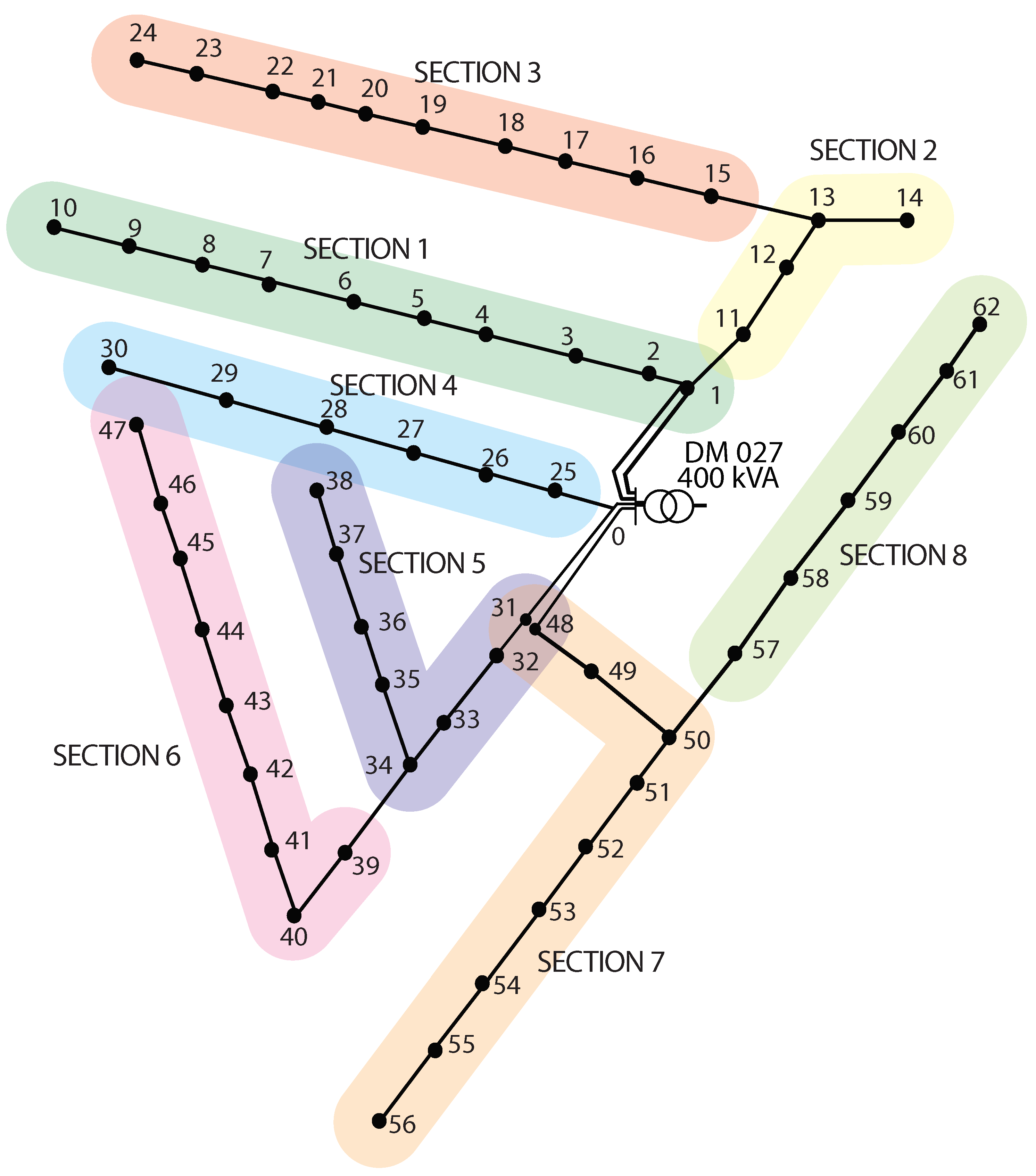
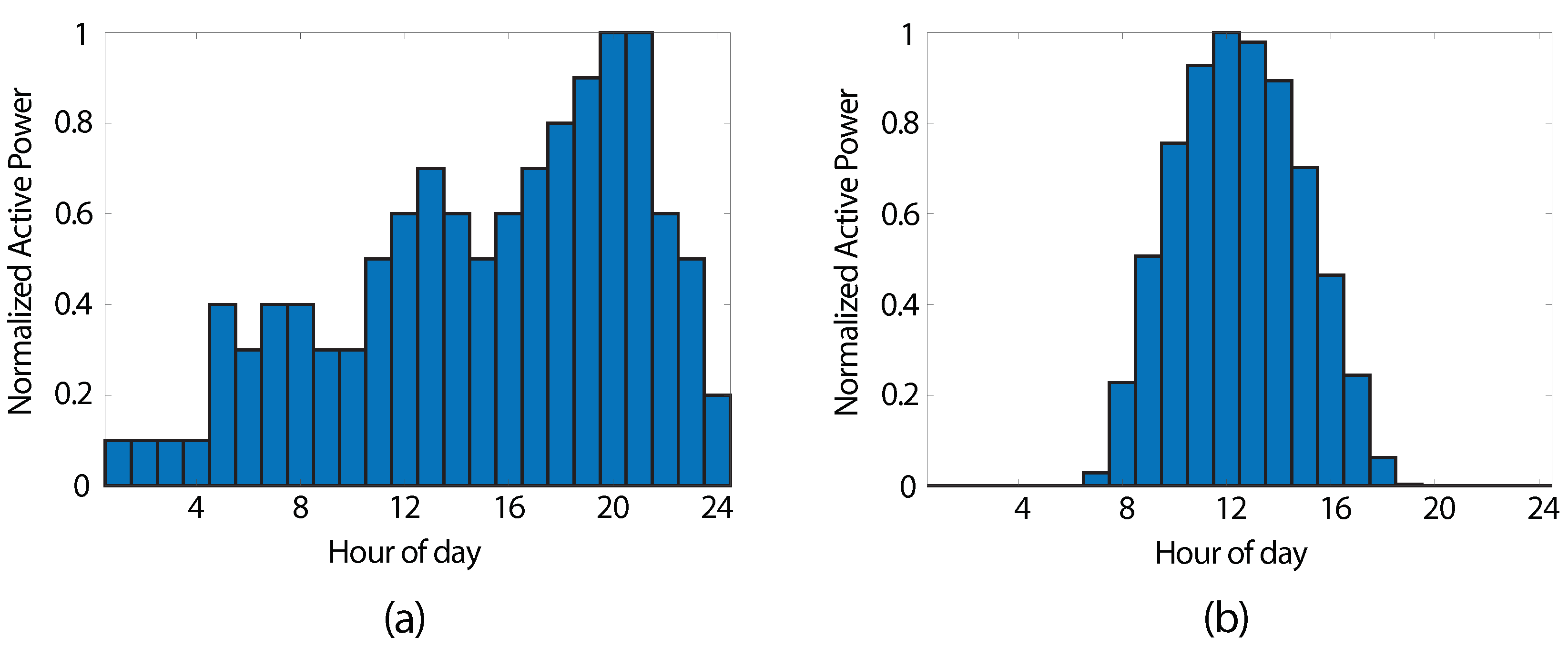
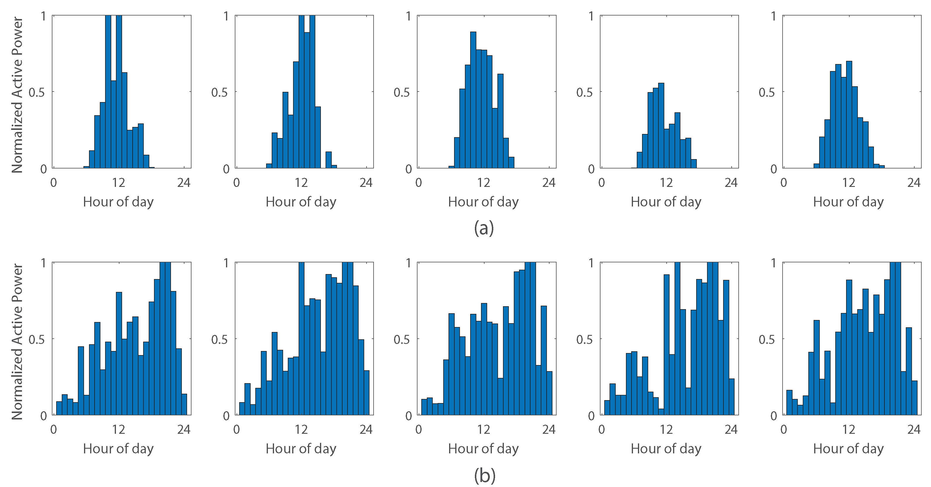
The steps involved in PSO are shown in Algorithm 1. The update equation for the position and velocity of the particles is given by,
x i [ j + 1 ] = x i [ j ] + V i [ j + 1 ]
where x i [ j ] denotes the position of the ith particle at the jth iteration and x i [ j + 1 ] and V i [ j + 1 ] are the position and velocity of that particle for the next iteration. The velocity at which the particle travels is expressed by,
V i [ j + 1 ] = V i [ j ] + P b ( p i [ j ] x i [ j ] ) + G b ( g [ j ] x i [ j ] )
where V i [ j ] is the velocity of the particle at the jth iteration, p i [ j ] and g [ j ] denote the current personal and global best of the jth particle and P b and G b are the confidence factors for the personal and global best, respectively.
The notion of the velocity is to set the direction of search and the extent of exploration by the particle. This depends on where in the search space the current particle exists, the recorded best position of that particle (personal best) and the recorded best position of all particles (global best) since the start of the algorithm. The dependency of the personal or global best on the velocity is governed by confidence factors, expressed by the two variables P b and G b .
To find the optimal values of the parameters P b and G b , an exhaustive search using the grid-search algorithm was carried out. Here, the ratio between P b and G b varied between 0.5 and 3 in steps of 0.5, and the number of iterations taken along with the final cost value was recorded. The magnitude of these parameters was set in the range of 0–1. It was found out that after FRS, as the particles were already scattered within the feasible region, each particle following its own local optima resulted in lower cost values for the final solution in most scenarios. Hence, more emphasis was given towards particles moving towards their own local optima rather than global optimum. Therefore, a 2:1 ratio between P b and G b was set during the optimization. This creates a wider net in the search space, thereby exploring many local minima. This increases the likelihood that the global minimum will be within this wide net.
To decrease the computational time whilst running the proposed two-stage optimization algorithm, the PSO population parameter needs to be optimized. Therefore, the convergence towards a feasible solution of the algorithm was recorded for initial populations varying from 5–50. Throughout the population search, it was observed that the optimization variable remained in the feasible region for all populations. Moreover, a population of 10 resulted in a significantly lower cost in comparison to an initial population of 5, whilst having a significantly lesser computational time compared to other population sizes. Hence, a population of 10 was chosen as the optimal population parameter for the PSO algorithm embedded in the proposed two-stage optimization.

5. Case Study

The network belonging to an existing housing complex “Lotus Grove” located in Colombo, Sri Lanka, was used as the case study. The network location also provides climatic variations of the tropical region. Its topology with 63 nodes is shown in Figure 8. The Number 0 node is the root node and connected to the secondary side of the MV-LV transformer. The rated capacity of the transformer is 400 kVA delta-wye, and the input/output voltage rating is 11 kV/415 V. The solid lines in Figure 8 represent the three-phase feeders where three-phase or single-phase loads and PV systems are connected. The overhead electricity distribution cable used is the aluminium aerial bundle cable (ABC-Al/XLPE of 3 × 70 + N54.6 + 1 × 16). There are 286 single-phase or three-phase customers and 50 PV panels connected to the network. The PV panel locations are uniformly distributed across the network with assigned ratings ranging from 2–7 kW and customer peak loads assigned in the range of 0.5–1 kW through a uniformly distributed assignment process. The daily operation curves for the PV systems and the daily load profile of customer loads used in the case study are shown in Figure 9. A few random load and PV profiles used in the case study are shown in Figure 10 to show the varying nature of the profiles evaluated. Images 1, 2 and 3 of Figure 10a represent sunny days that are randomly generated for a given PV panel, while Images 4 and 5 of Figure 10a represent cloudy days. Thus, these random generations encapsulate possible weather conditions that exist in a tropical environment.

6. Results and Discussion

To simulate the occurrences of upper and lower limit voltage violations, Monte Carlo (MC) simulations were run for three time instances. Since we intended to identify and mitigate voltage violations, the most prevalent cases for such violations were identified and Monte Carlo simulations were performed for these chosen times of the day: 10:00 h, 11:00 h and 21:00 h. This is due to the high PV power available between 10:00 h and 11:00 h, while the load is much less, leading to severe upper limit violations. Similarly, the load is maximum around 21:00 h while there is no PV power, leading to many lower limit violations. Since the violations occurring at other time instances were much less, they posed a much simpler problem to be solved. Therefore, showing the ability to solve the worst-case time instances confirmed the ability to handle the simpler violated cases. Table 2 describes the three instances in terms of the hour of simulation, the network settings (PV and load setting), the number of simulations and the number of control instances that employed reactive power control or active power control (RPC or APC) or both, to mitigate voltage violations.
As observed in Table 2, voltages at simulations carried out at 10:00 violated more often, due to the low base loading. However, they tended to have a higher possibility of mitigating the upper limit violations using only RPC Q-absorption. Comparatively, at 11:00, when PV penetration increases, the rectification cannot be solely performed via Q-absorption, as shown in Table 2; hence, a higher number of APC rectifications (Q-absorption followed by APC) took place. For the simulation at 21:00 (night-time), every simulation contained lower limit violations only, which was caused by full base loading. With a large number of simulations using randomly generated individual base loads, PV sources and PV positions in the network for each simulation, the robustness of the control algorithm under extreme circumstances was ensured.
To maintain computational consistency within this study, all simulations were run on an Intel i7-8700k processor with 16GB of RAM. All scripts and functions were written using MATLAB R2020a. Load flow computations were carried out using the OpenDSS interface with MATLAB.

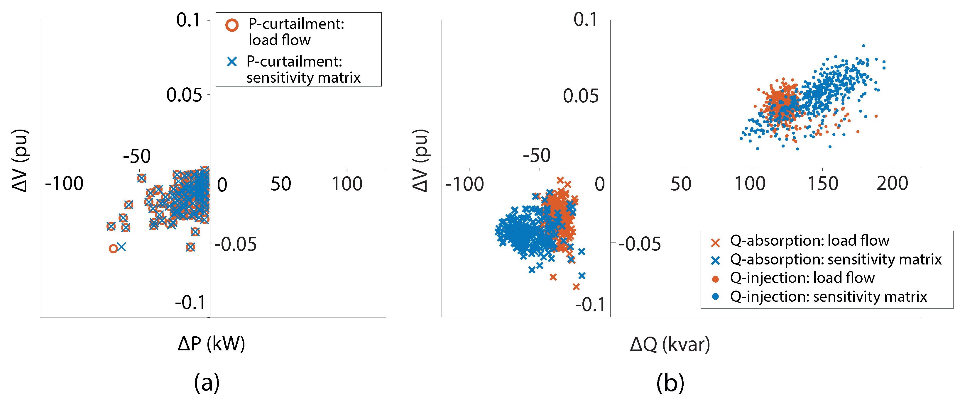
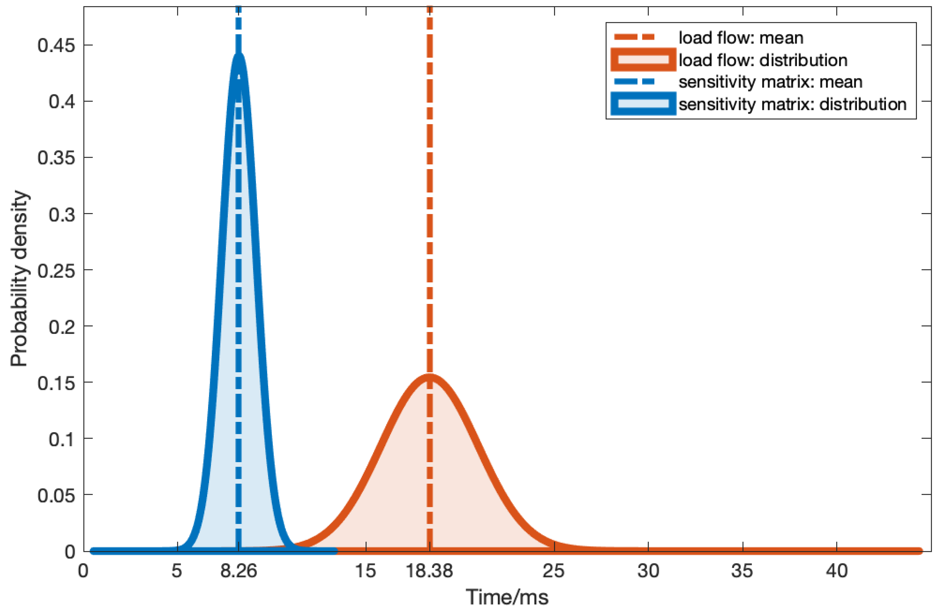
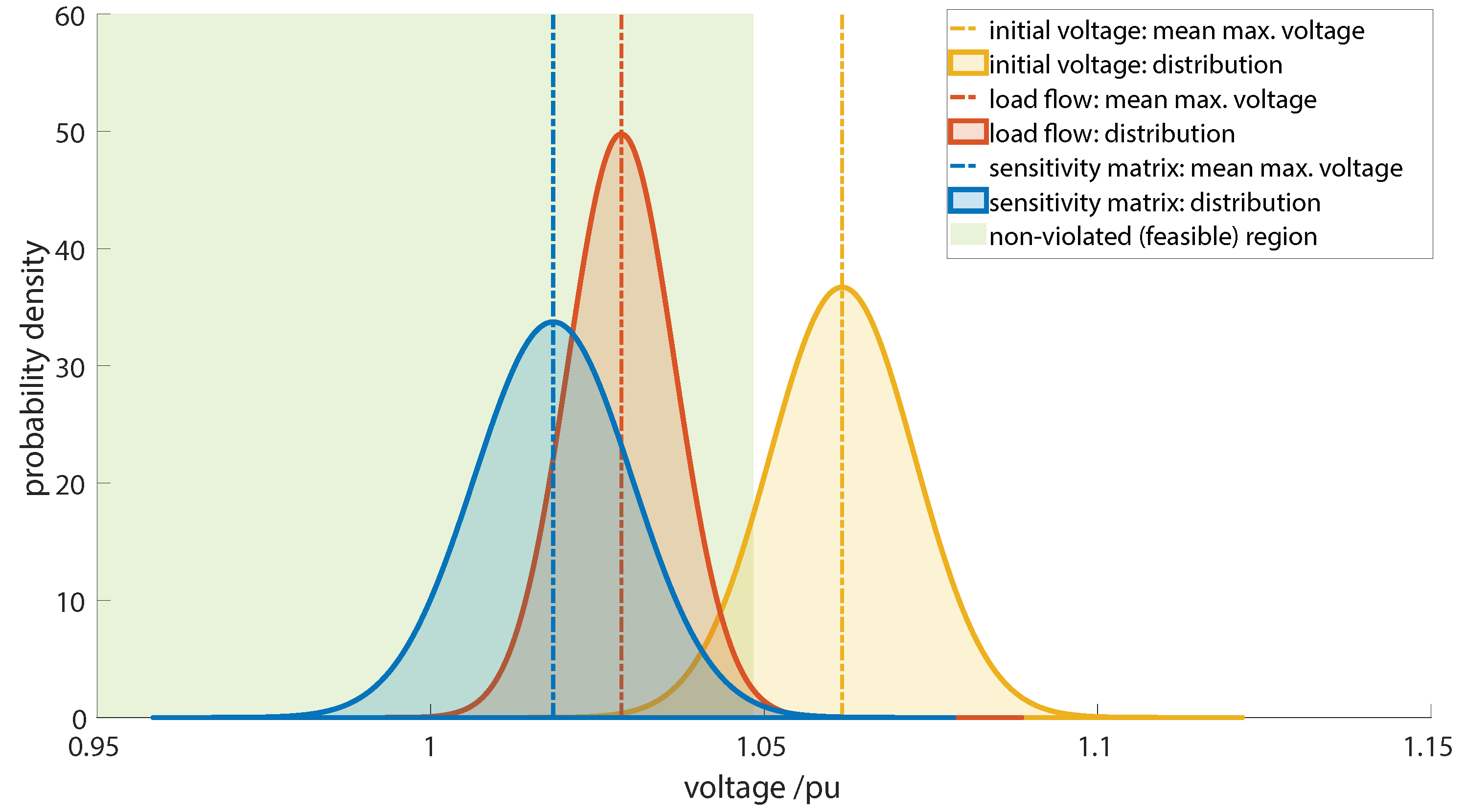
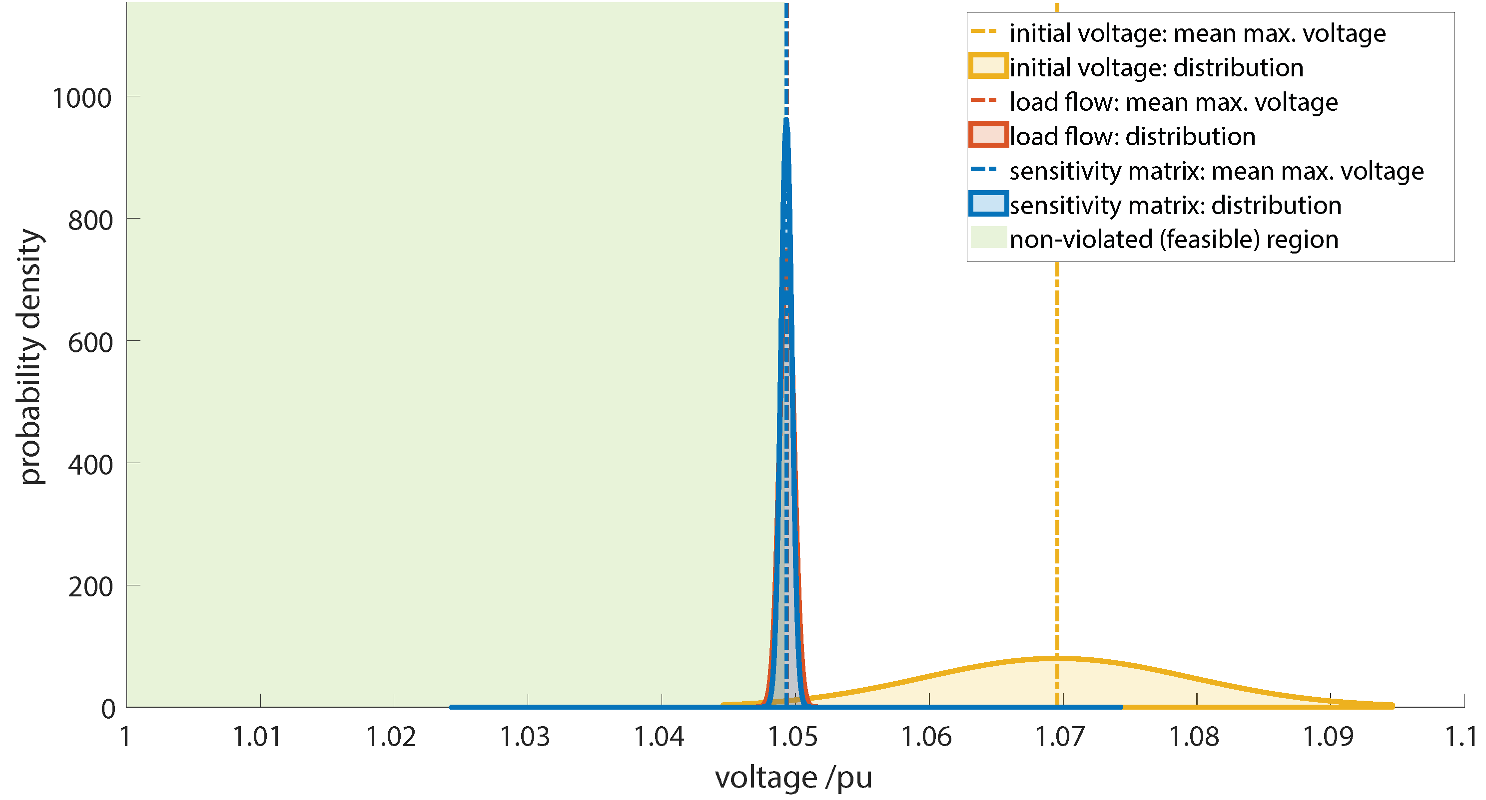
6.1. Validation of the Sensitivity Matrix

This section demonstrates the validity of the proposed sensitivity matrix for voltage sensitivity calculation for power injection/absorption/curtailment. The SM was analysed with respect to the load flow approach for the MC simulations discussed in Table 2 for the amount of power injected/absorbed/curtailed and the respective voltage change that was achieved. This is presented in Figure 11a for RPC and Figure 11b for APC, where each marker denotes the values after each MC simulation. The voltage change presented in this figure is for the worst violated node in each case where the deviation of the initial voltage is largest from 1 p.u. Therefore, the RPC Q-injection scenarios were analysed with respect to the node with the lowest voltage (less than 0.95 p.u) since it had lower limit violations, and the RPC Q-absorption scenarios were analysed with respect to the node with the highest voltage (greater than 1.05 p.u) since it had upper limit violations. APC was also analysed with respect to the node with the highest voltage, but in comparison to the active power used. The voltage profiles after the optimization using the load flow method and the SM method are further discussed in Section 6.3.
The amount of active power used in both methods was almost consistently the same in APC, as seen in Figure 11a. This is because the optimization was designed with a high penalty to the amount of active power curtailed. Therefore, it was FRS that greatly contributed to APC, as the FRS step drives the solution as close as possible to the feasible region and the PSO always ensures that the final solution has minimal active power curtailed, i.e., at the boundary of the feasible region.
Considering RPC, two distinct regions can be seen in Figure 11b. The RPC using Q-absorption reduced the voltage in the nodes by consuming reactive power, hence in the lower-left quadrant of the plane, whereas RPC using Q-injection lifted the voltage by supplying reactive power, hence on the top-right quadrant. It can be observed that the plots for both the SM and the load flow approach are very much overlapping. The SM can be seen to slightly overcompensate in reactive power usage in the range of 20–30 kVARs with a difference in the voltage change lying within 0.01 p.u.
While the SM overcompensates in reactive power usage, this difference is minimal in comparison to the computational time benefit of the SM over the load flow approach. The distribution of the computational times using the SM and the load flow for the MC simulations is shown in Figure 12. It can be observed that the SM approach converges to the solution with a time benefit of 55.1% for the mean computational time, as shown in Table 3.

6.2. Feasible Region Search for Optimization

Out of the 3000 MC simulations conducted for the Q-absorption and APC scenarios (as in Table 2), FRS was able to drive the O V to the feasible region devoid of any voltage violations. Meanwhile, in the 500 MC simulations conducted for the Q-injection scenarios, except for 35 simulations, FRS was again able to drive the O V to the feasible region devoid of any violations. Considering the 35 rare instances out of all simulation runs, FRS ensured that the O V was driven to the closest possible setting to the feasible region, ensuring that the PSO was able to converge to the optimal solution.
To demonstrate the effectiveness and necessity of FRS in the proposed two-stage optimization algorithm, 100 separate MC simulations were run with and without FRS. Within each MC simulation, the two-stage optimization and the standalone PSO were carried out for varying population sizes and initialization parameters, and the solutions were analysed.
In this study, the initialization parameter used was the scatter variance, which determines the spread of the PSO particles that are initially populated in the neighbourhood at the starting point. Increasing the population and scatter variance together increases the probability of these particles being closer to the optimal solution, due to a large number of particles in the initial population being spread over a vast area in the solution space. However, given a large solution space as in this study, standalone PSO does not always guarantee a solution in the feasible region even under the aforementioned initial conditions. These results are summarized in Table 4. Here, it was observed that on average, 34% of solutions obtained by standalone PSO did not fall under the feasible region. In contrast, when FRS was used with PSO, every scenario generated using the MC simulation resulted in the final solution being inside the feasible region, i.e., no violations. This shows the necessity of FRS in the optimization algorithm, where it effectively drives the optimization variable towards the solution, thus enabling PSO to carry out finer adjustments towards finding an optimal solution.
It can be noted that increasing the population slightly reduces the overall number of instances where the solution is unfeasible. However, it was observed that the average computational time per iteration increased linearly with the size of the population. Hence, an increase in the population size for PSO in order to optimize its performance will lead to higher computational time in reaching the solution, which is unfavourable for the problem.

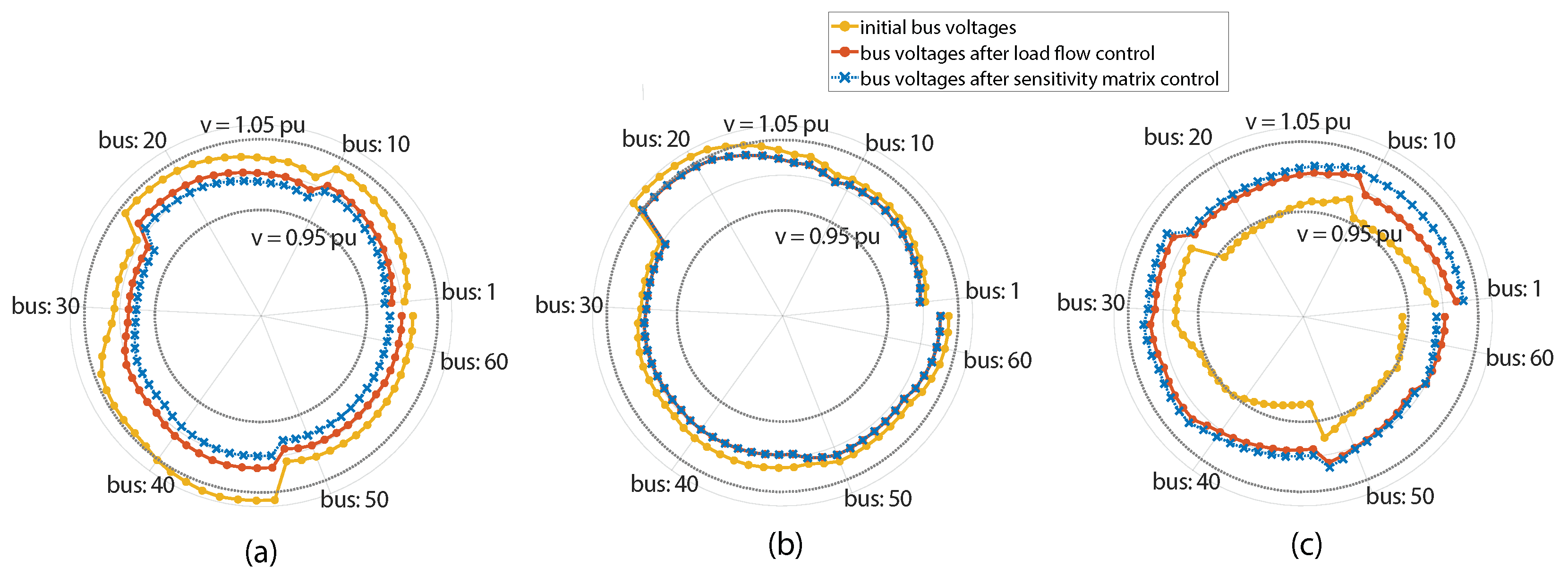
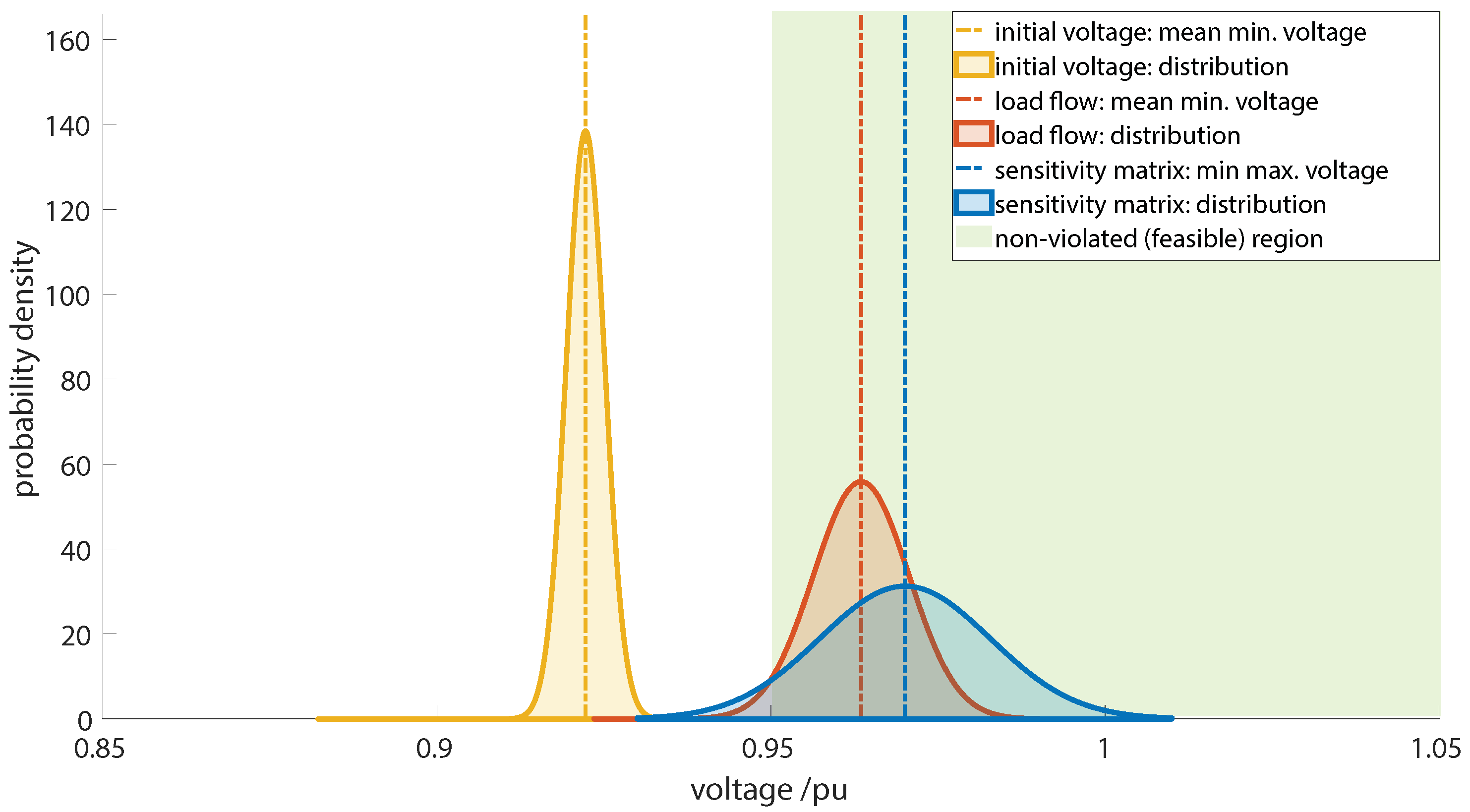
6.3. Two-Stage Optimization and Proposed Sensitivity Matrix

In order to create a considerable number of violations to emulate a possible worst-case scenario handling capability of the proposed SM method and to demonstrate its robustness, PV panel positions were randomly generated such that a relatively higher number of panels were connected to Phase 3, increasing the number of violations in that phase. Therefore, the initial and final voltages in the worst possible phase, Phase 3, after control using the SM approach and the load flow method, both using the two-stage optimization, are shown in Figure 13 for one particular simulation for each case at 10:00, 11:00 and 21:00.
The distribution of the minimum voltage of the set of nodes after RPC using Q-injection obtained using the 500 MC simulations conducted at 21:00 as per Table 2 is shown in Figure 14. Similarly, the distribution of the maximum voltage after Q-absorption obtained using 410 MC simulations (violated simulations) out of the 1000 simulations conducted at 10:00 as per Table 2 is shown in Figure 15. It can be observed that the lower limit violations and upper limit violations were successfully eliminated by the control sequences. There was a slight incremental shift of 6.5 × 10 3 p.u of the mean voltage in the minimum voltage distribution of the sensitivity matrix approach compared to the load flow approach after Q-injection (Figure 14). Similarly, the maximum voltage distribution of the sensitivity matrix method was slightly lower with a 1.02 × 10 2 p.u difference of the mean voltage compared to the load flow method (Figure 15). This was due to the overcompensation of power by sensitivity matrix due to its approximation, as described in Section 6.1. However, the optimization ensures that both methods successfully mitigate voltage violations while minimising the voltage deviations in each phase.
Finally, the APC algorithm is heavily dependent on the amount of active power curtailed rather than the voltage deviations in each phase. Hence, when the Q-absorption is not sufficient to remove the violations, APC is performed, which attempts to just remove the violation. Therefore, the maximum voltage of the set of nodes is always at 1.05 p.u (the upper limit). This is seen in Figure 16, which shows the distribution of the voltage profile obtained after APC, using the 102 MC simulations (violated simulations) out of 2000 simulations conducted at 11:00 as per Table 2. Hence, in the APC case, both the sensitivity matrix approach and the load flow approach yielded the exact same result.

7. Conclusions

In this paper, a novel Sensitivity Matrix (SM) and a Centralized Active Reactive Power Management System (CARPMS) using inverter control to eliminate voltage limit violations were introduced. The optimum PV power settings for the control sequence were determined by a novel modified two-stage optimization algorithm. The two-stage optimization algorithm takes the predicted PV power and the estimated node voltages as inputs to determine the PV inverter active and reactive power settings to eliminate the voltage violations whilst minimising the unbalance in the network.
To demonstrate the effectiveness of the proposed SM approach and the two-stage optimization algorithm, a simulation study was performed on an existing LV network. The effectiveness and necessity of the FRS combination with PSO (two-stage optimization) was analysed by running 100 Monte Carlo simulations with FRS and without FRS (using only PSO). It was observed that nearly 34% of the simulation scenarios were not solved by the PSO-only optimization to remove the voltage violations. It was further observed that there was considerable overlap as to which cases had violations after optimization when using PSO only. This confirmed that the PSO algorithm is unable to handle specific voltage violation scenarios regardless of the parameters being tuned. However, with the combination of FRS (the two-stage optimization), all the simulations were able to find a solution removing all violations. Furthermore, the two-stage optimization was able to find solutions with a population of only 10, which further reduced the computational time.
The two-stage optimization algorithm performance was first implemented using load flows and then using the SM for the voltage profile generation. The results showed that the SM is able to successfully assimilate the performance of the state-of-the-art solution: the load flow, in all cases of reactive power injection, reactive power absorption and active power curtailment. The difference between the mean voltages of the proposed methodology and the load flow methods were 6.5 × 10 3 p.u for RPC using Q-injection, 1.02 × 10 2 p.u for RPC using Q-absorption. It is noteworthy that the voltage profiles obtained after APC were exactly the same for both methods (0 p.u mean voltage difference), which reaffirmed the SM approach. Furthermore, the SM reduced the time consumed for the voltage profile generation by 55% when compared to the load flow method. This faster inverter control will mitigate voltage violations in LVDGs, thereby allowing utility providers to accommodate more rooftop solar panels into LV networks.
The main advantage of the proposed two-stage optimization using the SM is the reduction in time to generate the voltage profiles during the control sequence. Since the SM approach is able to perform the network voltage estimation with a 55% reduction in time with negligible accuracy loss, this will speed up the control of voltage violations in LVDGs. Furthermore, the CARPMS implementation’ initial cost is minimal due to the use of existing PV inverters without the need for additional device installation for the control operation.

Author Contributions

Conceptualization, A.S.J.H., U.M., G.W.K.P., A.B., W.G.C.B., P.B.E., R.I.G. and J.B.E.; methodology, A.S.J.H., U.M., G.W.K.P., A.B., P.B.E., R.I.G. and J.B.E.; software, A.S.J.H., U.M., G.W.K.P. and A.B.; validation, A.S.J.H., U.M., W.G.C.B., P.B.E., R.I.G. and J.B.E.; formal analysis, A.S.J.H., U.M., P.B.E., R.I.G. and J.B.E.; investigation, A.S.J.H. and U.M.; resources, P.B.E., R.I.G. and J.B.E.; data curation, G.W.K.P., A.B. and W.G.C.B.; writing—original draft preparation, A.S.J.H., U.M., G.W.K.P. and A.B.; writing—review and editing, A.S.J.H., U.M., W.G.C.B., P.B.E., R.I.G. and J.B.E.; visualization, A.S.J.H. and U.M.; supervision, W.G.C.B., P.B.E., R.I.G. and J.B.E.; project administration, A.S.J.H., U.M., P.B.E., R.I.G. and J.B.E.; funding acquisition, P.B.E., R.I.G. and J.B.E. All authors have read and agreed to the published version of the manuscript.

Funding

This research was funded by the National Science Foundation (NSF), Sri Lanka, Research Grant Numbers RG/2018/EA and ICT/01, and the Peradeniya Engineering Faculty Alumni Association (PEFAA).

Institutional Review Board Statement

Not applicable.

Informed Consent Statement

Not applicable.

Conflicts of Interest

The authors declare no conflict of interest. The funders had no role in the design of the study; in the collection, analysis, or interpretation of data; in the writing of the manuscript; nor in the decision to publish the results.

References

  1. U.S. Energy Information Administration. Annual Energy Outlook. Available online: https://www.eia.gov/outlooks/aeo/ (accessed on 6 November 2020).
  2. Almeida, D.W.; Abeysinghe, A.H.M.S.M.S.; Ekanayake, J.B. Analysis of rooftop solar impacts on distribution networks. Ceylon J. Sci. 2019, 48, 103–112. [Google Scholar] [CrossRef] [Green Version]
  3. Hamilton, J.; Negnevitsky, M.; Wang, X.; Lyden, S. High penetration renewable generation within Australian isolated and remote power systems. Energy 2019, 168, 684–692. [Google Scholar] [CrossRef]
  4. Colantuono, G.; Kor, A.L.; Pattinson, C.; Gorse, C. PV with multiple storage as function of geolocation. Sol. Energy 2018, 165, 217–232. [Google Scholar] [CrossRef] [Green Version]
  5. Walling, R.A.; Saint, R.; Dugan, R.C.; Burke, J.; Kojovic, L.A. Summary of Distributed Resources Impact on Power Delivery Systems. IEEE Trans. Power Deliv. 2008, 23, 1636–1644. [Google Scholar] [CrossRef]
  6. Akeyo, O.M.; Patrick, A.; Ionel, D.M. Study of Renewable Energy Penetration on a Benchmark Generation and Transmission System. Energies 2021, 14, 169. [Google Scholar] [CrossRef]
  7. Ma, C.; Dasenbrock, J.; Töbermann, J.C.; Braun, M. A novel indicator for evaluation of the impact of distributed generations on the energy losses of low voltage distribution grids. Appl. Energy 2019, 242, 674–683. [Google Scholar] [CrossRef]
  8. Tonkoski, R.; Turcotte, D.; EL-Fouly, T.H.M. Impact of High PV Penetration on Voltage Profiles in Residential Neighborhoods. IEEE Trans. Sustain. Energy 2012, 3, 518–527. [Google Scholar] [CrossRef]
  9. Chaminda Bandara, W.; Godaliyadda, G.; Ekanayake, M.; Ekanayake, J. Coordinated photovoltaic re-phasing: A novel method to maximize renewable energy integration in low voltage networks by mitigating network unbalances. Appl. Energy 2020, 280, 116022. [Google Scholar] [CrossRef]
  10. Ma, C.; Menke, J.H.; Dasenbrock, J.; Braun, M.; Haslbeck, M.; Schmid, K.H. Evaluation of energy losses in low voltage distribution grids with high penetration of distributed generation. Appl. Energy 2019, 256, 113907. [Google Scholar] [CrossRef]
  11. Yaghoobi, J.; Islam, M.; Mithulananthan, N. Analytical approach to assess the loadability of unbalanced distribution grid with rooftop PV units. Appl. Energy 2018, 211, 358–367. [Google Scholar] [CrossRef]
  12. Almeida, D.; Abeysinghe, S.; Ekanayake, M.P.; Godaliyadda, R.I.; Ekanayake, J.; Pasupuleti, J. Generalized approach to assess and characterise the impact of solar PV on LV networks. Int. J. Electr. Power Energy Syst. 2020, 121, 106058. [Google Scholar] [CrossRef]
  13. Aziz, T.; Ketjoy, N. PV penetration limits in low voltage networks and voltage variations. IEEE Access 2017, 5, 16784–16792. [Google Scholar] [CrossRef]
  14. Shahnia, F.; Majumder, R.; Ghosh, A.; Ledwich, G.; Zare, F. Voltage imbalance analysis in residential low voltage distribution networks with rooftop PVs. Electr. Power Syst. Res. 2011, 81, 1805–1814. [Google Scholar] [CrossRef]
  15. Hashemi, S.; Østergaard, J.; Degner, T.; Brandl, R.; Heckmann, W. Efficient Control of Active Transformers for Increasing the PV Hosting Capacity of LV Grids. IEEE Trans. Ind. Inform. 2017, 13, 270–277. [Google Scholar] [CrossRef] [Green Version]
  16. Yorino, N.; Zoka, Y.; Watanabe, M.; Kurushima, T. An Optimal Autonomous Decentralized Control Method for Voltage Control Devices by Using a Multi-Agent System. IEEE Trans. Power Syst. 2015, 30, 2225–2233. [Google Scholar] [CrossRef]
  17. Christakou, K.; Paolone, M.; Abur, A. Voltage Control in Active Distribution Networks Under Uncertainty in the System Model: A Robust Optimization Approach. IEEE Trans. Smart Grid 2018, 9, 5631–5642. [Google Scholar] [CrossRef]
  18. Payne, J.; Gu, F.; Razeghi, G.; Brouwer, J.; Samuelsen, S. Dynamics of high penetration photovoltaic systems in distribution circuits with legacy voltage regulation devices. Int. J. Electr. Power Energy Syst. 2021, 124, 106388. [Google Scholar] [CrossRef]
  19. Xie, Q.; Shentu, X.; Wu, X.; Ding, Y.; Hua, Y.; Cui, J. Coordinated voltage regulation by on-load tap changer operation and demand response based on voltage ranking search algorithm. Energies 2019, 12, 1902. [Google Scholar] [CrossRef] [Green Version]
  20. Chen, C.; Lin, C.; Hsieh, W.; Hsu, C.; Ku, T. Enhancement of PV Penetration With DSTATCOM in Taipower Distribution System. IEEE Trans. Power Syst. 2013, 28, 1560–1567. [Google Scholar] [CrossRef]
  21. Arshad, A.; Püvi, V.; Lehtonen, M. Monte Carlo-based comprehensive assessment of PV hosting capacity and energy storage impact in realistic finnish low-voltage networks. Energies 2018, 11, 1467. [Google Scholar] [CrossRef] [Green Version]
  22. Zhao, B.; Ren, J.; Chen, J.; Lin, D.; Qin, R. Tri-level robust planning-operation co-optimization of distributed energy storage in distribution networks with high PV penetration. Appl. Energy 2020, 279, 115768. [Google Scholar] [CrossRef]
  23. Ma, Y.; Azuatalam, D.; Power, T.; Chapman, A.C.; Verbič, G. A novel probabilistic framework to study the impact of photovoltaic-battery systems on low-voltage distribution networks. Appl. Energy 2019, 254, 113669. [Google Scholar] [CrossRef]
  24. Alzahrani, A.; Alharthi, H.; Khalid, M. Minimization of power losses through optimal battery placement in a distributed network with high penetration of photovoltaics. Energies 2020, 13, 140. [Google Scholar] [CrossRef] [Green Version]
  25. Mak, D.; Choi, D.H. Hierarchical look-ahead conservation voltage reduction framework considering distributed energy resources and demand reduction. Energies 2018, 11, 3250. [Google Scholar] [CrossRef] [Green Version]
  26. Al-Saffar, M.; Musilek, P. Reinforcement Learning-Based Distributed BESS Management for Mitigating Overvoltage Issues in Systems With High PV Penetration. IEEE Trans. Smart Grid 2020, 11, 2980–2994. [Google Scholar] [CrossRef]
  27. Tonkoski, R.; Lopes, L.A.C.; El-Fouly, T.H.M. Coordinated Active Power Curtailment of Grid Connected PV Inverters for Overvoltage Prevention. IEEE Trans. Sustain. Energy 2011, 2, 139–147. [Google Scholar] [CrossRef]
  28. Tonkoski, R.; Lopes, L.A. Impact of active power curtailment on overvoltage prevention and energy production of PV inverters connected to low voltage residential feeders. Renew. Energy 2011, 36, 3566–3574. [Google Scholar] [CrossRef] [Green Version]
  29. Alyami, S.; Wang, Y.; Wang, C.; Zhao, J.; Zhao, B. Adaptive Real Power Capping Method for Fair Overvoltage Regulation of Distribution Networks With High Penetration of PV Systems. IEEE Trans. Smart Grid 2014, 5, 2729–2738. [Google Scholar] [CrossRef]
  30. Howlader, A.M.; Sadoyama, S.; Roose, L.R.; Chen, Y. Active power control to mitigate voltage and frequency deviations for the smart grid using smart PV inverters. Appl. Energy 2020, 258, 114000. [Google Scholar] [CrossRef]
  31. Latif, A.; Gawlik, W.; Palensky, P. Quantification and mitigation of unfairness in active power curtailment of rooftop photovoltaic systems using sensitivity based coordinated control. Energies 2016, 9, 436. [Google Scholar] [CrossRef] [Green Version]
  32. Nousdilis, A.I.; Christoforidis, G.C.; Papagiannis, G.K. Active power management in low voltage networks with high photovoltaics penetration based on prosumers’ self-consumption. Appl. Energy 2018, 229, 614–624. [Google Scholar] [CrossRef]
  33. Weckx, S.; Gonzalez, C.; Driesen, J. Combined Central and Local Active and Reactive Power Control of PV Inverters. IEEE Trans. Sustain. Energy 2014, 5, 776–784. [Google Scholar] [CrossRef]
  34. Ghosh, S.; Rahman, S.; Pipattanasomporn, M. Local distribution voltage control by reactive power injection from PV inverters enhanced with active power curtailment. In Proceedings of the 2014 IEEE PES General Meeting| Conference & Exposition, Washington, DC, USA, 27–31 July 2014; IEEE: New York, NY, USA, 2014; pp. 1–5. [Google Scholar]
  35. Calderaro, V.; Conio, G.; Galdi, V.; Massa, G.; Piccolo, A. Optimal Decentralized Voltage Control for Distribution Systems With Inverter-Based Distributed Generators. IEEE Trans. Power Syst. 2014, 29, 230–241. [Google Scholar] [CrossRef]
  36. Zhu, H.; Liu, H.J. Fast Local Voltage Control Under Limited Reactive Power: Optimality and Stability Analysis. IEEE Trans. Power Syst. 2016, 31, 3794–3803. [Google Scholar] [CrossRef]
  37. Wang, X.; Wang, C.; Xu, T.; Guo, L.; Li, P.; Yu, L.; Meng, H. Optimal voltage regulation for distribution networks with multi-microgrids. Appl. Energy 2018, 210, 1027–1036. [Google Scholar] [CrossRef]
  38. Gandhi, O.; Zhang, W.; Rodríguez-Gallegos, C.D.; Verbois, H.; Sun, H.; Reindl, T.; Srinivasan, D. Local reactive power dispatch optimisation minimising global objectives. Appl. Energy 2020, 262, 114529. [Google Scholar] [CrossRef]
  39. Tina, G.M.; Garozzo, D.; Siano, P. Scheduling of PV inverter reactive power set-point and battery charge/discharge profile for voltage regulation in low voltage networks. Int. J. Electr. Power Energy Syst. 2019, 107, 131–139. [Google Scholar] [CrossRef]
  40. Jabr, R.A. Robust Volt/VAr Control With Photovoltaics. IEEE Trans. Power Syst. 2019, 34, 2401–2408. [Google Scholar] [CrossRef]
  41. Zhang, Z.; Dou, C.; Yue, D.; Zhang, B.; Zhao, P. High-economic PV power compensation algorithm to mitigate voltage rise with minimal curtailment. Int. J. Electr. Power Energy Syst. 2021, 125, 106401. [Google Scholar] [CrossRef]
  42. Zhang, Q.; Dehghanpour, K.; Wang, Z. Distributed CVR in Unbalanced Distribution Systems With PV Penetration. IEEE Trans. Smart Grid 2019, 10, 5308–5319. [Google Scholar] [CrossRef]
  43. Emarati, M.; Barani, M.; Farahmand, H.; Aghaei, J. A two-level over-voltage control strategy in distribution networks with high PV penetration. Int. J. Electr. Power Energy Syst. 2021, 130, 106763. [Google Scholar] [CrossRef]
  44. Cheng, Z.; Li, Z.; Liang, J.; Si, J.; Dong, L.; Gao, J. Distributed coordination control strategy for multiple residential solar PV systems in distribution networks. Int. J. Electr. Power Energy Syst. 2020, 117, 105660. [Google Scholar] [CrossRef]
  45. Singh, S.; Pamshetti, V.B.; Thakur, A.K.; Singh, S. Multistage multiobjective volt/var control for smart grid-enabled CVR with solar PV penetration. IEEE Syst. J. 2020, 15, 2767–2778. [Google Scholar] [CrossRef]
  46. Ilea, V.; Bovo, C.; Falabretti, D.; Merlo, M.; Arrigoni, C.; Bonera, R.; Rodolfi, M. Voltage control methodologies in active distribution networks. Energies 2020, 13, 3293. [Google Scholar] [CrossRef]
  47. Wang, L.; Yan, R.; Saha, T.K. Voltage regulation challenges with unbalanced PV integration in low voltage distribution systems and the corresponding solution. Appl. Energy 2019, 256, 113927. [Google Scholar] [CrossRef]
  48. Nguyen, H.M.; Torres, J.L.R.; Lekić, A.; Pham, H.V. MPC Based Centralized Voltage and Reactive Power Control for Active Distribution Networks. IEEE Trans. Energy Convers. 2021, 36, 1537–1547. [Google Scholar] [CrossRef]
  49. Marikkar, U.; Hassan, A.S.J.; Maithripala, M.S.; Godaliyadda, R.I.; Ekanayake, P.B.; Ekanayake, J.B. Modified Auto Regressive Technique for Univariate Time Series Prediction of Solar Irradiance. In Proceedings of the 2020 IEEE 15th International Conference on Industrial and Information Systems (ICIIS), Rupnagar, India, 26–28 November 2020; IEEE: New York, NY, USA,, 2020; pp. 22–27. [Google Scholar]
  50. Chaminda Bandara, W.G.; Almeida, D.; Godaliyadda, R.I.; Ekanayake, M.P.; Ekanayake, J. A complete state estimation algorithm for a three-phase four-wire low voltage distribution system with high penetration of solar PV. Int. J. Electr. Power Energy Syst. 2021, 124, 106332. [Google Scholar] [CrossRef]
  51. Degefa, M.; Lehtonen, M.; Millar, R.; Alahäivälä, A.; Saarijärvi, E. Optimal voltage control strategies for day-ahead active distribution network operation. Electr. Power Syst. Res. 2015, 127, 41–52. [Google Scholar] [CrossRef] [Green Version]
  52. Su, X.; Masoum, M.A.S.; Wolfs, P.J. Optimal PV Inverter Reactive Power Control and Real Power Curtailment to Improve Performance of Unbalanced Four-Wire LV Distribution Networks. IEEE Trans. Sustain. Energy 2014, 5, 967–977. [Google Scholar] [CrossRef]
  53. Jung, J.; Onen, A.; Arghandeh, R.; Broadwater, R.P. Coordinated control of automated devices and photovoltaic generators for voltage rise mitigation in power distribution circuits. Renew. Energy 2014, 66, 532–540. [Google Scholar] [CrossRef]
  54. Ma, W.; Wang, W.; Chen, Z.; Wu, X.; Hu, R.; Tang, F.; Zhang, W. Voltage regulation methods for active distribution networks considering the reactive power optimization of substations. Appl. Energy 2021, 284, 116347. [Google Scholar] [CrossRef]
  55. Yang, H.; Liao, J. MF-APSO-Based Multiobjective Optimization for PV System Reactive Power Regulation. IEEE Trans. Sustain. Energy 2015, 6, 1346–1355. [Google Scholar] [CrossRef]
  56. Mahmoud, K.; Lehtonen, M. Three-level control strategy for minimizing voltage deviation and flicker in PV-rich distribution systems. Int. J. Electr. Power Energy Syst. 2020, 120, 105997. [Google Scholar] [CrossRef]
  57. Su, X.; Masoum, M.A.S.; Wolfs, P. Comprehensive optimal photovoltaic inverter control strategy in unbalanced three-phase four-wire low voltage distribution networks. IET Gener. Transm. Distrib. 2014, 8, 1848–1859. [Google Scholar] [CrossRef]
  58. Samadi, A.; Shayesteh, E.; Eriksson, R.; Rawn, B.; Söder, L. Multi-objective coordinated droop-based voltage regulation in distribution grids with PV systems. Renew. Energy 2014, 71, 315–323. [Google Scholar] [CrossRef]
  59. Zhu, X.; Wang, J.; Mulcahy, D.; Lubkeman, D.L.; Lu, N.; Samaan, N.; Huang, R. Voltage-load sensitivity matrix based demand response for voltage control in high solar penetration distribution feeders. In Proceedings of the 2017 IEEE Power & Energy Society General Meeting, Chicago, IL, USA, 16–20 July 2017; IEEE: New York, NY, USA, 2017; pp. 1–5. [Google Scholar]
  60. Zhang, Z.; Ochoa, L.F.; Valverde, G. A novel voltage sensitivity approach for the decentralized control of DG plants. IEEE Trans. Power Syst. 2017, 33, 1566–1576. [Google Scholar] [CrossRef] [Green Version]
  61. Zad, B.B.; Hasanvand, H.; Lobry, J.; Vallée, F. Optimal reactive power control of DGs for voltage regulation of MV distribution systems using sensitivity analysis method and PSO algorithm. Int. J. Electr. Power Energy Syst. 2015, 68, 52–60. [Google Scholar]
  62. Chen, Y.; Strothers, M.; Benigni, A. All-day coordinated optimal scheduling in distribution grids with PV penetration. Electr. Power Syst. Res. 2018, 164, 112–122. [Google Scholar] [CrossRef]
  63. Ge, X.; Shen, L.; Zheng, C.; Li, P.; Dou, X. A Decoupling Rolling Multi-Period Power and Voltage Optimization Strategy in Active Distribution Networks. Energies 2020, 13, 5789. [Google Scholar] [CrossRef]
  64. Alboaouh, K.; Mohagheghi, S. Voltage and power optimization in a distribution network with high PV penetration. In Proceedings of the 2018 IEEE/PES Transmission and Distribution Conference and Exposition (T&D), Denver, CO, USA, 16–19 April 2018; IEEE: New York, NY, USA, 2018; pp. 1–9. [Google Scholar]
  65. De Din, E.; Pau, M.; Ponci, F.; Monti, A. A Coordinated Voltage Control for Overvoltage Mitigation in LV Distribution Grids. Energies 2020, 13, 2007. [Google Scholar] [CrossRef] [Green Version]
  66. Ferreira, W.M.; Meneghini, I.R.; Brandao, D.I.; Guimarães, F.G. Preference cone based multi-objective evolutionary algorithm to optimal management of distribuited energy resources in microgrids. Appl. Energy 2020, 274, 115326. [Google Scholar] [CrossRef]
  67. Jain, N.; Singh, S.; Srivastava, S. Particle Swarm Optimization Based Method for Optimal Siting and Sizing of Multiple Distributed Generators. In Proceedings of the 16th National Power Systems Conference, Hyderabad, India, 15–17 December 2010; pp. 669–674. [Google Scholar]
  68. Resources. Available online: https://site.ieee.org/pes-testfeeders/resources/ (accessed on 1 August 2021).
  69. Boglou, V.; Karavas, C.S.; Arvanitis, K.; Karlis, A. A fuzzy energy management strategy for the coordination of electric vehicle charging in low voltage distribution grids. Energies 2020, 13, 3709. [Google Scholar] [CrossRef]
  70. Fu, C.; Wang, C.; Wang, L.; Zhao, B. Control of PV systems for distribution network voltage regulation with communication delays. Electr. Power Syst. Res. 2020, 179, 106071. [Google Scholar] [CrossRef]
  71. Welikala, S.; Dinesh, C.; Ekanayake, M.P.B.; Godaliyadda, R.I.; Ekanayake, J. A real-time non-intrusive load monitoring system. In Proceedings of the 2016 11th International Conference on Industrial and Information Systems (ICIIS), Roorkee, India, 3–4 December 2016; pp. 850–855. [Google Scholar]
  72. Welikala, S.; Thelasingha, N.; Akram, M.; Ekanayake, P.B.; Godaliyadda, R.I.; Ekanayake, J.B. Implementation of a robust real-time non-intrusive load monitoring solution. Appl. Energy 2019, 238, 1519–1529. [Google Scholar] [CrossRef]
  73. Welikala, S.; Dinesh, C.; Ekanayake, M.P.B.; Godaliyadda, R.I.; Ekanayake, J. Incorporating Appliance Usage Patterns for Non-Intrusive Load Monitoring and Load Forecasting. IEEE Trans. Smart Grid 2019, 10, 448–461. [Google Scholar] [CrossRef]
  74. Dinesh, C.; Welikala, S.; Liyanage, Y.; Ekanayake, M.P.B.; Godaliyadda, R.I.; Ekanayake, J. Non-intrusive load monitoring under residential solar power influx. Appl. Energy 2017, 205, 1068–1080. [Google Scholar] [CrossRef]
  75. Fang, Z.; Lin, Y.; Song, S.; Song, C.; Lin, X.; Cheng, G. Active distribution system state estimation incorporating photovoltaic generation system model. Electr. Power Syst. Res. 2020, 182, 106247. [Google Scholar] [CrossRef]
  76. Wang, C.; Wu, J.; Ekanayake, J.; Jenkins, N. Smart Electricity Distribution Networks; CRC Press: Boca Raton, FL, USA, 2017. [Google Scholar]
Figure 1. Hierarchical control architecture.
Energies 14 06596 g001
Figure 2. Schematic overview of the CARPMS information flow.
Energies 14 06596 g002
Figure 3. Proposed algorithm steps.
Energies 14 06596 g003
Figure 4. A schematic LVDG network.
Energies 14 06596 g004
Figure 5. Equivalent circuit of the delta-wye transformer.
Energies 14 06596 g005
Figure 6. PV inverter status change for control using (a) Q-absorption, (b) Q-absorption and P-curtailment and (c) Q-injection.
Energies 14 06596 g006
Figure 7. Effect of α on FRS.
Energies 14 06596 g007
Figure 8. Single line diagram of the test LVDG network (Lotus Grove, Sri Lanka) used for the simulations.
Energies 14 06596 g008
Figure 9. Daily (a) load profile and (b) PV profile.
Energies 14 06596 g009
Figure 10. Random (a) PV profiles for a single PV panel and (b) load profiles for a single customer used in the case study.
Energies 14 06596 g010
Figure 11. Change in reactive/active power and the corresponding voltage change in the most violated node for (a) reactive power control and (b) active power curtailment.
Energies 14 06596 g011
Figure 12. Comparison of computational time for the load flow and SM approaches.
Energies 14 06596 g012
Figure 13. Voltage profiles of Phase 3 before and after control at (a) 10:00 using Q-absorption, (b) 11:00 using Q-absorption and P-curtailment and (c) 21:00 using Q-injection.
Energies 14 06596 g013
Figure 14. Distribution of minimum controlled voltages after Q injection obtained using MC simulations at 21:00.
Energies 14 06596 g014
Figure 15. Distribution of maximum controlled voltages after Q absorption obtained using MC simulations at 10:00.
Energies 14 06596 g015
Figure 16. Distribution of maximum controlled voltages after P curtailment obtained using MC simulations at 11:00.
Energies 14 06596 g016
Table 1. Sensitivity matrices existing in the literature.
How the Sensitivity Matrix Was DevelopedReferencesDisadvantages of the Method
Inverse from the Jacobian of Newton–Raphson power flow equations[27,58]Repetitive computation of the inverse of the Jacobian, which is computationally expensive with the increase in matrix size.
Surface fitting technique and using simulations of multiple load flow analysis[59,60]An extensive simulation needs to be run in case of a change in the network parameters to be able to develop a new sensitivity matrix that will fit the network.
Using the topological structure of the network[61]The derivation is performed for an MV distribution line assuming constant voltage for the slack bus. However, the secondary voltage of the LV network will fluctuate, which needs to be accounted for.
Table 2. Monte Carlo simulations.
Time of DayPV SourceBase LoadNumber of Simulation RunsControl Instances
RPC Q-absAPCRPC Q-inj
10:0076%30%100040370
11:0093%50%20003251020
21:000%100%50000500
Table 3. Elapsed computational time for sensitivity matrix and load flow calculation.
Calculation MethodComputational Time/s
MeanStd. DeviationMinimumMaximum
Load Flow18.382.5814.7544.38
Sensitivity Matrix8.260.905.3512.10
Table 4. Percentage of unfeasible solutions after standalone PSO for varying population size and scatter variance.
PopulationScatter Variance
0.10.20.51.02.0
54141454546
103838384041
203330303333
303030292930
502827272828
Publisher’s Note: MDPI stays neutral with regard to jurisdictional claims in published maps and institutional affiliations.

