
Power Quality Phenomena, Standards, and Proposed Metrics for DC Grids


Department of Electrical, Electronics and Telecommunication Engineering and Naval Architecture (DITEN), University of Genova, 16145 Genova, Italy
Energies 2021, 14(20), 6453; https://doi.org/10.3390/en14206453
Submission received: 1 August 2021
/
Revised: 15 September 2021
/
Accepted: 15 September 2021
/
Published: 9 October 2021
(This article belongs to the Collection Feature Papers in Smart Grids and Microgrids)
Abstract
:This work addresses the problem of power quality (PQ) metrics (or indexes) suitable for DC grids, encompassing low and medium voltage applications, including electric transports, all-electric ships and aircrafts, electric vehicles, distributed generation and microgrids, modern data centers, etc. The two main pillars on which such PQ indexes are discussed and built are: (i) the physical justification, so the electric phenomena affecting DC grids and components (PV panels, fuel cells, capacitors, batteries, etc.), causing, e.g., stress of materials, aging, distortion, grid instability; and (ii) the existing standardization framework, pointing out desirable coverage and extension, similarity with AC grids standards, but also inconsistencies. For the first point, each phenomenon is discussed with quantitative conclusions on relevant thresholds: in many cases some percentage of distortion (ripple) is acceptable (stress on capacitors and storage, impact on fuel cells, and PV panels), whereas in other cases, much higher levels may be tolerated (interference to protection and monitoring devices). Standards are reviewed for indications not only of low-order harmonics and voltage fluctuations typical of old DC grid schemes, but also for high-frequency noise, including thus supraharmonics and common-mode disturbance, and filling the gap with the electromagnetic compatibility domain. However, phenomena typical of EMC and electrical safety (such as various types of overvoltages and fast transients) are excluded. Suitable PQ indexes are then reviewed, suggesting integrations and modifications, to cover the relevant phenomena and technological progress, and to better follow the normative exigencies: ripple is considered in time and frequency domain, in particular with a band limited implementation; for transients and pulsed loads, more traditional indexes based on area, energy, and half duration are confronted with indexes evaluating the power trajectory and its derivative.
1. Introduction
The term “DC grid” encompasses various types of distribution networks that are extensively used for a wide range of applications, distinguishing between grids (large physical extension and/or integrated with the national and trans-national grids), microgrids, and down to nanogrids. Such networks are operated both at medium voltage (MV) and low voltage (LV) with some standardized nominal values and variable physical extension: from some meters to tens of meters within a large room, a smart house, or an electrified vehicle; hundreds of meters between buildings, at a campus, or on-board ships; up to some km for distribution within smart residential districts, technological parks, etc.; or several tens to thousands of km for electrified transportation systems, such as tramways, metros, and railways. Long distances are reached with high-voltage DC transmission links, that are, however, outside the scope of this work.
The application of DC grids has recently grown faster than the development and update of suitable complete standards; a discussion of the standardization framework is thus necessary, in view of the various DC grids architectures, of the electrical phenomena that characterize them, and the effect of such phenomena on the grid elements.
DC microgrids in one of their simplest implementations have been used for a long time for backup and high-availability circuits (such as to allow black start of power generation facilities, data centers, laboratories with mission critical or sensitive applications, etc.) and have always been quite diffused on-board vehicles and boats. Today, higher integration of sources and loads and better dynamic performances can be attributed to the robustness, simplicity, and availability just exemplified. The power and voltage levels have also correspondingly shifted from low values (as provided by 12, 24, 48, 60, and 110 Vdc circuits) to ratings comparable to AC grids, made possible by the development of semiconductor devices and converter architectures (370–400 V for data centers, up to about 800 V for residential distribution, and 600 to 3000 V for electric transports, several kV for MV distribution). The relevant features are increased switching frequency, increased voltage and current ratings, high efficiency, bidirectional power flow, and control of distortion and of low-frequency electromagnetic interference (EMI).
The proliferation of microgrids, nanogrids, and smart grids fully exploits the flexibility and performance of converters and control, interconnecting a wide range of sources and loads. The increase of the installed power has shifted the nominal voltages to higher values, for both AC and DC grids, despite the intrinsic difficulty of protection of the latter for short circuit [1,2,3] and series arc phenomena [4,5,6]. Correspondingly, the physical extension has grown, requiring significant synchronization and control capabilities. MV is necessary for large power concentrations, such as photo-voltaic (PV) and wind parks [7], as well as distribution on-board ships [8,9].
On-board ships, various types of loads (first of all the propulsion load, but also electromagnetic weapons, special cargo services such as refrigeration, etc.) are connected with different dynamics and power absorption levels. Short-circuit protection for MV DC systems is always a challenge and several static DC breaker architectures have been proposed [10,11], in addition to the more consolidated air and vacuum breakers [12]. The extension of the network amounts to some hundreds of meters (accounting for ship length and some branching and routing). The installed power is in the range of several MW to tens of MW. The number of static converters has also increased to compartmentalize pulsed loads and disturbing loads, to services and more susceptible systems, possibly fed at lower voltage level [13]. For disturbance mitigation, the use of filters and capacitance to ground (i.e., to the ship hull) is subject to restrictions, in order to limit common mode current injection.
Another example of MV DC grid consists of DC railways [14,15] and rapid transit systems, featuring dynamic moving loads, all supplied from a catenary (or third rail) system fed by rectifier substations. These networks feature the largest extension, as they cover entire cities, regions, and countries. Such electric distribution grids feature a peculiar arrangement of conductors with a larger line inductance, but lower capacitance compared to cable distribution, for which resonance frequencies are not so different, whereas the factor of merit and the excursion of network impedance values are much larger [16].
LV networks are more diffused and may be found on-board ships (when, e.g., large loads of propulsion are separated), aircrafts and trains, as well as serving technological and residential centers and integrating various types of sources and loads [13] (sources including in particular photo-voltaic (PV) panels and fuel cells, as well described for telecommunications and data centers in the ETSI TR 102 532 [17]). The physical extension for an LV grid is in general limited to a few km [18].
For smart grids and microgrids, one of the advantages of DC distribution is the ease of integration of sources and loads, without the complication of phase angle instability and coordination, typical of AC applications. A short physical extension is in the order of some tens or hundreds of meters, which brings resonances in the frequency interval of the typical emissions of interfaced converters. This aspect has recently attracted a lot of interest and research, studying EMC problems of the so-called supraharmonic 9–150 kHz interval [19]. The use of interface filters of LCL type may help reduce the problem, although they increase the likeliness of resonances at lower frequency, especially if some devices are interfaced with CLC filters (such as the omnipresent EMI filters) [20].
The primary quantity in all distribution networks is the voltage at equipment terminals: DC grids, compared to AC grids, have lower harmonic distortion thanks to larger capacitance and in general lower harmonic impedance, as shown in [21], comparing harmonic power terms in AC and DC railways. A lower harmonic impedance, however, amplifies current distortion that will flow mostly in filter capacitors and capacitor banks, with consequential overheating, stress, and aging. Energy storage devices are in general interfaced by means of DC/DC converters and are thus decoupled. In general, current, in addition to voltage, should be evaluated for the following reasons:
- high-performance control uses information on current not only to improve performance with feed-forward control, but also to control impedance [22];
- distorted current is a cause of induced disturbance through cables, in particular for common-mode components that are often the result of large capacitance to ground (as resulting either by the distributed capacitance of the source or load, such as PV panels or battery banks, or by purposely inserted capacitors to reduce EMI) [20]; common-mode current is not evaluated by the commonly used PQ indexes, being usually ascribed to EMC, and those uncontrolled common-mode currents, aside from interference, may also increase the overall human exposure to magnetic field right where limits are particularly low [37];
- distorted current may also directly cause disturbance for specific signaling systems using the return circuit or ground wire as an active conductor; examples may be found in metros and railways (track circuits using the running rails as part of a coded signal transmission to detect the presence of trains) and in the automotive sector (negotiation of the charging profile of an electric vehicle following SAE J2836-1 [38] and IEC 61851-1 [39] standards, using pulse-width-modulated signals).
At high frequency in the supraharmonics interval and beyond, the network response becomes more complex and the impedance is generally higher, similar to the AC distribution for a similar cable implementation. A significant distortion is expected from the widespread use of converters and suitable assessment methods may be the same in use for AC distribution; in fact, the line impedance stabilization networks (also called artificial networks) are largely the same for AC and DC networks for the frequency intervals 9–150 kHz and 0.15–30 MHz.
This paper aims at providing a comprehensive picture of power quality (PQ) in DC grids, going beyond previous works [13,40,41], including a discussion of impact on DC grid elements (sources, loads, storage, protections), and considering the actual standardization framework for a punctual and harmonized contribution. This paper is thus organized as follows.
Section 2 describes the relevant network phenomena that justify a quantification of the related PQ, going into the details of EMC and distortion issues, correct operation of protection and monitoring devices, impact of transients on the DC grid stability considering low- and high-frequency oscillations, and aspects of stress and aging of connected devices (in particular filtering and storage devices).
Section 3 proposes instead a PQ classification based on standards, discussing in some cases inconsistencies and incomplete definitions, and hinting at suitable PQ metrics. Measurement and post-processing methods are only briefly described, when common to AC grids and well-disciplined in the available normative. PQ metrics can be broadly classified as related to small variations, around a nominal value, and large variations, as caused by faults and transients; going from the former to the latter, the identified metrics can be enumerated as distortion, ripple, area, energy, and power trajectory, discussed in this order in Section 4. Real cases and examples are sometimes considered to support the discussion, but there is no specific fifth section of detailed analysis for a matter of space.
2. Relevant Power Quality Phenomena
The definition of useful and suitable PQ indexes for DC grids in a wide perspective needs to begin with the identification of the typical and relevant PQ phenomena and events, and how they affect grid elements: sources, loads, connecting components, and control [42]. PQ events affect these elements in various ways with different consequences and time scales, which by similarity with AC distribution networks may be enumerated as follows:
- interference to sources and loads as an EMC (electromagnetic compatibility) problem, affecting e.g., measurement and control quantities;
- interference to sources and loads as an operational problem, resulting in poor voltage quality (fluctuations and variations) disrupting source or load operation, causing flicker, torque variation, etc.; in this respect, DC grids intrinsically perform better thanks to a large amount of local storage;
- issues of network instability and low-frequency oscillations (LFOs), in particular when stressed by major transients, that trigger undamped response of sources and loads; by convention, LFOs in AC networks are confined below the fundamental; here, without loss of generality, LFO may be considered to occur up to a hundred Hz;
- resonances occurring at higher frequency (often named high-frequency oscillations, HFO, or harmonic resonances, HR), above usual control bandwidths, related to network resonances, influenced by the physical extension and interaction with parasitics and reactive elements; and
- impact in terms of overheating and accelerated aging, as for filter capacitors, cables, storage devices, and transformer insulation; ripple current and in general the rms value and the number of charging/discharging cycles are the parameters of the electrical interface considered for quantification of stress and aging of batteries and supercapacitors, in addition to environmental conditions and in particular temperature.
PQ indexes in AC networks have historically covered similar issues, with limits defined about 30 years ago. A similar approach is pursued here, on the one hand exploiting experience and knowledge of such PQ AC indexes, and on the other focusing on components and characteristics peculiar of modern DC grids in their various applications.
For a matter of clarity, when referring generally to low, medium, and high frequency for conducted disturbance, the intention is to consider frequency intervals up to some kHz (that can be fixed at 2 or 9 depending on the adopted standard), up to 150 kHz (or slightly beyond, such as 500 kHz, for practical reasons), and up to 30 MHz, respectively.
2.1. EMC and Interference
PQ phenomena may represent a source of interference for connected equipment and its control systems. As an EMC problem it is correctly addressed focusing on both weakness (or susceptibility) of victim equipment and the way the disturbance couples from the source to the victim.
Modern equipment has an increased level of EM immunity, guaranteed nowadays by compliance to quite developed EMC standards with wide application. The focus should, then, be on phenomena still poorly covered in the standards and on intrinsic susceptibility, for example, related to a specific function, especially for communication devices, such as power line communication (or power line carrier, PLC).
Historically, notches and harmonic disturbances in AC networks were identified that could affect converter synchronization and control (e.g., accuracy of mains zero-crossing detection), which is not relevant in case of DC applications. Modern protection relays, encompassing residual current devices (RCDs), leakage current monitoring, arc fault detection devices (AFDDs), or equivalently arc fault circuit interrupters (AFCIs), related algorithms for arc detection, and systems for predictive DC fault current interruption in large-power installations, are all potentially exposed to distortion and noise due to the processing of current and voltage high-frequency content (aiming at effective detection and fast triggering):
- Residual current devices (RCDs), a class of devices common to AC and DC applications, relying on current measurements for detection of fault conditions with a wide range of fault impedance values. Type B of AC RCDs could be used for DC applications, although they are not fully specified for it; such devices may have an unspecified sensitivity to high-frequency components [43,44]. Conversely, RCDs for DC applications are required to be immune from high-frequency ripple (see section 8.17 in [45]), but the amplitude and frequency of such ripple are not better specified. Coordinated solutions are being proposed complementing the limited immunity of single devices to a wide range of disturbance with an increased information set collected by distance protections and networked devices [46].
- DC leakage monitors: the latest IEC 62020-1 [47] does not yet include DC devices, but they are covered by the EN 61557-8 [48], considering their application to “pure DC IT systems”. Practically speaking, a pure DC IT grid does not exist as some amount of differential- and common-mode ripple is always present. Such devices have been available on the market for a long time (such as Bender [49], Danisense [50] or THIIM [51] brands) with sensitivities that expose them to unwanted tripping, as caused by current ripple, that may also occur on the earth conductors due to unavoidable potential difference between remote locations (in particular when switching power converters are used). In some cases, a selectable filter [50] allows to limit the bandwidth, but the real susceptibility to high-frequency ripple is rarely declared, nor disciplined by any kind of standard. Personal experience with one of these devices indicates susceptibility (and unwanted tripping at the DC threshold of about 10 mA) in the range 50–70 mArms for ripple occurring at some kHz.
- Series arcs detection methods [4,52]. The method in [4] is based on the comparison of current drop estimates in successive short time intervals (50 μs) and with running average values on longer intervals (50 ms), showing a factor of 2 of difference in the indicators with and without arc; the required sampling is 200 kSa/s, thus potentially exposed to high-frequency pollution from static converters, then reduced by successive averaging. Similarly, in [53], min and max current values are run over optimized window lengths (5 to 25 ms), whose difference is an indicator of intermittence; the influence of system noise was not investigated, although the number of consecutive windows used in estimates can be used to filter out grid transients such as load steps, avoiding them being detected as arcs. A much lower sampling of 1440 Sa/s is required in [52], thus less exposed to system noise and high-frequency switching components. Commercially available AFDDs/AFCIs are mainly focused on AC grids (the EN 62606 [54] considers only AC distribution, whereas the UL 1699B [55] specifically addresses arcs in DC grids and PV systems), but the extensive deployment of PV systems has fostered the design of some specific devices [56,57]. The detection method is not detailed, but the monitored frequency range is reported as above 20 kHz [57] and between 20 and 40 kHz [56]. In both cases, this detection range would be exposed to distortion from the AC network (for transformerless PV systems), transient responses to, e.g., step changes [58], and most of all to supraharmonics originating from converters, as it is evident in [56], where the 16 kHz-spaced switching harmonics have almost the same amplitude of the targeted arc noise (and there are cases of noise profiles dominated by such harmonic peaks). Tests of effectiveness and performance indicated by the UL 1699B include a change of distance from the arc to detect (farther by 66 m) to check sensitivity and the verification of correct operation with an inverter connected. A quantitative framework would be welcome, specifying the minimum signal-to-noise ratio with respect to supraharmonics, that should be in any case subject to limitations.
- DC protections for large-power installations are implemented as assisted circuit breakers (called “hybrid”) [11] or fully static semiconductor-based devices [10], driven by detection algorithms. Various techniques have been proposed and applied to DC railways [3,59] and distributed generation DC grids [60,61], exploiting various methods and monitored grid quantities: (i) methods based on autonomous signal injection and impedance estimation [3,59] are rather immune to distortion, as ideally, the applied intensity may increase until a satisfactory operation is achieved; (ii) the criterion proposed for the DC side of a wind power system in [60] is based on DC ripple, that in normal conditions must be low (0.2%) for the method to work; (iii) the robust technique correlating internal current waveforms to separate faults of internal and external origin [61] was tested against uncorrelated Gaussian noise, but not with signal distortion, which is highly correlated as well.
PLC systems use power conductors as a communication means and are potentially exposed to equipment-conducted emissions of differential type. For AC networks, PLC may be subdivided into long-haul communication (occurring at high voltage and involving distribution and transmission substations) and a range of medium- and short-haul systems providing telemetry, telecommunication, and data exchange services over a broad frequency range for, e.g., tariff application and optimization, metering, distributed control, and diagnostics. These systems exploit both the medium frequency range up to 500 kHz (for example, CENELEC bands exploit up to 122 kHz, whereas FCC pushes up to 487 kHz) and a higher MHz range, suitable for broadband over power line (BPL) applications. Such techniques may be considered straightforwardly applicable to DC grids, as the characteristics of cables in terms of attenuation and transmission are similar and the physical extension of a DC grid is in general limited. Focusing on PQ and disturbance rather than the suitability of DC grid architectures, a general concern regarding the noise margin for reception levels is well grounded.
In fact, although there are no limits of supraharmonic emissions from DC equipment, the typical emission limits in the EN 55014-1 [62] may be considered as a minimum reference level. Using then the test case shown in Figure 6 of [63], it is easy to see that the 66 to 56 dB·μV quasi-peak limit between 150 and 500 kHz translates into −64 to −74 dBm/Hz, having used the 200 Hz resolution bandwidth. The signal-to-noise margin is thus 10 dB with respect to the G3-PLC received signal plotted in [63], not accounting for the quasi-peak to peak value transformation (that is usually in the order of some dB up to about 10 dB). The typical noise of the studied DC grid with a resistive load instead is comparable or larger than the received signal, with peaks of an underlying modulation with 16 kHz pattern (the interface converter providing the DC supply) well above by about 10 dB. It has been observed that the PLC modem used for the tests (Devolo G3-PLC 500k [64]) has an output power of only −9 dBm at 50 Ω (0.1 Vrms) and there is margin to increase it with a design update up to the maximum of about 3.1 Vrms allowed by the EN 50065-1 [65]. This is almost compulsory for electric vehicle charging applications, where the limit of conducted emissions at the vehicle-charger interface is set to industrial environment levels and above, at 79, 100, and 130 dB·μV quasi-peak for ≤20 kVA, >20 kVA and ≤20 kVA, and >75 kVA of rated power, respectively [66].
Considering, therefore, the sum of the disturbance of many EN 55014-1 compliant devices sharing the same grid or the specific disturbance of interface AC/DC converter and other DC/DC converters (e.g., serving loads and storage devices), the amount of noise may affect the signal-to-noise ratio significantly, as shown in Figure 8 of [63], which just focuses on a very limited number of connected devices. As a consequence, a balanced and comprehensive limitation of emissions in the supraharmonic range is a necessity to allow the smooth operation of PLC technology in modern DC microgrids and smart grids. An effective approach is the adoption of spread-spectrum modulation converters, as shown in [67].
For other types of equipment, there remains a general concern of EMI that may be addressed by using the immunity test levels as reference. Distortion phenomena may propagate in differential mode (the most common and traditionally considered), but also in common mode. The IEC 61000-4-17 [68] addresses the differential-mode coupling onto the DC port of equipment, but the IEC 61000-4-16 [69] is quite relevant for common-mode disturbance on an extended frequency range. Such standards are, however, rarely recalled by product and application standards, so they remain largely voluntary. The IEC 61000-4-16 focuses on the frequency range up to 150 kHz, immediately beneath the IEC 61000-4-6. This test is justified by the widespread use of switching power converters and the propagation along interconnecting cable screens and armors, as well as other conductive parts (such as cable trays and ladders). Nevertheless, such converters can also cause differential-mode distortion affecting network quantities beyond the traditional limit of 2–2.5 kHz for harmonics. Propagation of both common- and differential-mode disturbance is favored by interaction and resonances between network capacitance and local equipment filters (e.g., EMI filters, and by extension all filters, feature both Cy, common mode, and Cx, differential mode, capacitors).
It has been observed that in DC grid applications, there is in principle no limitation for Cy capacitors (except for the 75 nF/kW figure of MIL-STD-461 [70], discussed in Section 3.5), whereas it is extensively applied in AC networks to limit the zero-sequence current leakage. A larger capacitance value implies a better control of EMI directed outside but a larger common-mode current injection in the local ground connection, possibly exposed to amplification caused by resonances of the real installation (occurring also in case of compliant equipment if taken alone).
From this, the relevance of suitable PQ indexes to weight the amount of distortion and spectral pollution for both differential and common-mode circuits, that allow also the evaluation of the incremental effect of new equipment and filters, can be determined [20].
2.2. Voltage Fluctuations and Variations
The terms “voltage fluctuation” and “voltage variation” are often used interchangeably, with some standards using only the former (EN 50155) or the latter (MIL STD 704), and possibly associating variation with ripple. We may say that voltage fluctuations and variations may be defined as slow changes of the network voltage within or exceeding, respectively, the stated tolerance values of the nominal voltage. In addition, the term “variation” is sometimes associated the concept of a faster behavior, although a clear distinction is not agreed on.
Voltage fluctuations in general affect the delivered amount of power and are responsible for a change of the reference quantities used by control systems. The straightforward compensation is possible either by means of local control of each source and load (as it is commonplace, but cannot operate beyond ratings), or by an external support, using storage devices and DC springs [71].
For some sources, fluctuations are intrinsic to the physical principle of energy generation, such as with PV and wind systems: clouds, environmental temperature and change of isolation during the day for the former, mainly change of wind speed and direction for the latter.
In general, DC systems are characterized by a wider range of variation of the network voltage compared to AC systems of similar power rating, as pointed out in Section 3.1. Even small DC systems fed by batteries (e.g., for backup or mobile applications) must consider the network voltage increase during recharging (usually amounting to +20/30%). A voltage variation, then, is the normal DC grid reaction to a load step and to inrush phenomena (see Section 3.3), for which standards specify a range of immunity tests for equipment against overvoltages and undervoltages of variable duration (detailed in Section 3.1). In electrified transportation lines at isolation points of catenary or third rail, the line voltage has a step change when crossing the discontinuity and is accompanied by arcing phenomena that might also have a peculiar spectral signature, as shown in [72].
2.3. Network Instability, Oscillations, and Resonances
Network instability and resonance are analyzed in the following, devising PQ indexes that are capable of monitoring, tracking, and possibly indicating incipient resonance conditions for prevention purposes.
The phenomenon is periodic and the apparent characteristic is the increase of the amplitude of one or few components (accompanied as a consequence by a slight increase of the overall rms value). Traditionally, the attention has been focused on high-frequency resonances. As observed in [73], the total harmonic distortion is not a good indicator, as low-order harmonics with higher amplitude would mask the distortion increase at higher frequencies, so that it is more effective to calculated band-limited THD indexes, such as with a filter bank approach or using intervals of selected indexes of the DFT. The consequence of resonances is the local increase of distortion (a first stress factor for components, as discussed below in Section 2.4) and the significant increase of the peak network voltage, causing undue stress and out-of-rating operation for components and equipment. Excessive peak voltage is in general at the origin of untimely triggering of protecting relays and permanent damage to surge protecting devices (SPDs) [74].
The interaction of distributed sources and loads through the grid may cause instability and oscillations that are usually classified as high-frequency oscillations (HFOs) and low-frequency oscillations (LFOs).
2.3.1. High-Frequency Oscillations (HFOs)
HFOs are caused by resonant conditions of the infrastructure, accounting for inductance and capacitance in the various grid elements: cables, converters and their filters, etc. They are common to all networks that contain a significant amount of reactive elements, and in particular in case of large physical extension, where resonances occur at lower frequency with a corresponding lower damping, as losses are lower (e.g., skin effect and dielectric losses). Moreover, for a small grid with limited inductance and capacitance of the connecting cables, HFOs may occur in the frequency interval of major converters emissions. Voltage-controlled and current-controlled converters (for example, interfacing distributed generators, DG) may be modeled by the parallel combination of the series impedance Zs and parallel admittance Yp of their equivalent circuits, respectively, including the impedance of connecting cables. As demonstrated in [75] and applied to DC grids in [29], where the two curves Zs and 1/Yp cross each other and the phase difference approaches 180°, the Nyquist condition is met for sustained oscillations and instability. This usually occurs in the interval of hundreds of Hz to some kHz, distinguishing a first resonance fr1 where Zs is inductive and 1/Yp is capacitive, followed by a second one (fr2) with the opposite behavior about a decade above. The first resonance fr1 is generally characterized by a large value of Zs that has only started its decreasing slope to intersect the increasing 1/Yp curve, and is thus of the oscillating voltage type. Conversely, the second resonance fr2 will see much lower impedance values with amplification of the current. Resonance frequencies may be excited by a wide range of phenomena of both transient and steady nature: load step within the dc grid, step reduction in the generators also within the grid, harmonics of the connected generators and loads, or voltage sags/swells from outside the DC grid through the interface converters. The second intersection is located at some kHz or a ten of kHz in the supraharmonic range.
The discussed effects are summarized in Table 1.
2.3.2. Low-Frequency Oscillations (LFOs)
LFOs, instead, are the result of instability of the combined action of sources, loads, and storage devices with their control systems. A significant research effort is trying to define rules and methods for the control of stability following, e.g., load step changes, allowing reconfiguration of the network with inclusion of new energy sources without major changes of the existing control algorithms [29]. Typical oscillation frequencies are in the range of some Hz to some tens of Hz. Several factors can bring the oscillations to lower frequency: electromechanical oscillations (in particular with hybrid AC/DC grids, embedding ac motors as for diesel generators, turbines and micro-turbines), the extension of the system (with longer cable connections), the power rating of the connected apparatus (lower impedance values and lower dynamics) and the behavior of constant power loads (CPLs), and by extension distributed generation operated in constant power dispatch mode and maximum power point tracking mode (electrically behaving as CPLs [76]). LFOs typically occur in the Hz to tens of Hz range, as shown for the hybrid AC/DC systems including wind farms and HVDC link [77] and AC machines [78].
In microgrids, voltage control by droop-controlled sources is exposed to low-frequency resonance frequencies with low damping, which is sometimes improved by interposing passive elements that increase damping, resulting however in poorer control performance and lower system efficiency [79]. Active damping methods are more attractive, but necessitate a more careful design, especially for robustness with respect to various microgrid topologies and the introduction of new sources and loads, or storage elements. The strategy followed in [79], for example, is that of clustering the zeros of the sources’ local control in the resulting microgrid overall transfer function, so that adding or removing one source will not affect the migration of network poles. A minimum damping strategy for each controller is also followed, so that when microgrid structural changes occur, the worst case of zero series impedance is already included and covered by adequate damping.
LFOs result in poorer network response to load steps and changes of operating conditions, perceived as a fluctuating network voltage by connected loads, leading in some extreme cases to out-of-range values. From a PQ index viewpoint with a monitoring and supervision objective, such oscillations may be detected by ripple estimate in an approximate frequency range of 1 to 100 Hz (see Section 3.4.3).
2.4. Stress, Heating, and Aging of Components
There is general agreement that the stress of components (capacitors, batteries, cables) is mainly related to overheating, which is in turn led back to the rms or ripple of the flowing current. Indirectly, for batteries and capacitors, network voltage values steadily above the nominal values for which these storage elements have been rated may lead to “dielectric stress”, and design margins should include this aspect. Overheating (with higher operating temperature and evaporation of materials) is the most relevant factor causing accelerated aging of components.
2.4.1. Capacitors
In general, capacitors for DC link and power applications may be subdivided into [80]: aluminum electrolytic capacitors (Al-caps), metallized polypropylene film capacitors (MPPF-caps), and multi-layer ceramic capacitors (MLCC or MLC-caps). The major failure mechanisms are synthesized in [80], sec. III.A, identifying as the “most critical stressors” temperature, voltage, and current for Al-caps, but only temperature and voltage for the other two types. The reason is a significantly larger equivalent series resistance (ESR) for the former and a lower tolerated ripple current.
Power dissipation contributions are two: dielectric losses and ohmic losses (related to the ESR); the latter is usually the largest for high-quality dielectrics [81]. The two terms have, in general, an opposite behavior with respect to capacitance: capacitors with larger capacitance have lower dielectric losses but higher ESR losses. Focusing on dielectric, higher stress occurs when the peak value of the inner electric field is larger.
In [82], relevant factors were identified for non-polarized dielectrics (cross-link poly ethylene, XLPE, and polypropylene, PP): the amount of harmonic content in terms of rms, but also the maximum peak value of the electric field, and the rate of change of the electric field, which are synthesized by the following indexes Kp, Krms, and Ks.
These indexes clarify three concepts:
- the peak value of the electric field (or voltage) indicates the stress on dielectric;
- the total rms value compared to the fundamental weights the overall distortion of the waveform and this is applicable in general to voltage and current;
- components at higher frequency cause additional heating not only for more pronounced skin effect in conductors (and possibly proximity effect), but also increased dielectric losses, and this is indicated by Ks; this index was derived focusing on the impact of signals with a large derivative, weighting thus each component by its harmonic order; the harmonic order h is in general recognized as related to increased power losses, although they do not go necessarily linearly with h.
Relative to voltage components, the flowing current increases with frequency as the capacitive reactance decreases; in addition, self heating causes a change of resistivity and dielectric dissipation factor. Capacitor manufacturers weight all these factors to determine the stress on their components and the expected life [83]. The general empirical expression reported in [80] is
where:
L and L0 are the lifetime under actual the use conditions and as tested, respectively;
V and V0 are the voltage at use condition and as tested, respectively;
T and T0 are the temperature in Kelvin at use condition and as tested;
Ea is the activation energy;
KB is the Boltzmann’s constant (8.62 × 10⁻⁵ eV/°K); and
n is the voltage stress exponent.
The voltage V in this formula is a steady DC value, deprived of distortion, ripple, and transients. The reason for such expression involving the activation energy and Boltzmann’s constant is the underlying use of the law of Arrhenius.
For ceramic materials, the values of Ea and n are in the range of 1.2–1.5 and 1.5–7, respectively [80]; the highest values of n are for new technologies using thinner dielectric layers. A similar relationship is shown for Al-caps in [84] with n ranging from 1 to 6.
For electrolytic capacitors, a known simplification of the general Expression (1) is achieved assuming a 125 °C temperature range ΔT and observing that
resulting in two influencing terms (the so-called “lifetime multipliers”), one depending on voltage and one on the temperature change.
The effect of current ripple is included as heating [85] caused by ESR and dissipation factor (D or tanδ), that have opposite temperature dependency: where the former reduces with increasing temperature by about 1–2%/°C [86], the latter has a moderate increase of about 0.3–0.4%/°C. Knowing the thermal parameters of the capacitor, the ripple quantity can be related to a temperature increase, and thus included in the lifetime equation.
where Ir,f0 indicates a reference ripple current at a given frequency f0, usually selected at the two ends of the band, namely 100/120 Hz or 100 kHz.
For the calculation of expected life, pragmatically, Nichicon [86] and Rubycon [87] (among other manufacturers) tabulate a frequency factor Kf that weights the relevance of a component to ESR value with respect to a reference frequency, in the present case, 100 kHz (in other cases, also 100 Hz or 120 Hz, the typical ripple of a single-phase diode rectifier, may be taken as reference). Values are shown in Figure 1. The most relevant variation occurs in the first decade of frequency, with Kf almost doubling for the lowest capacitance values and increasing by 10–20% for the largest values. Aluminum capacitors of higher voltage rating (i.e., 100 to 400 V) have higher values of ESR and their increase with frequency is less relevant: Kf increases by 30% in the first decade of frequency at 1 kHz and another 10–15% going up to 10 kHz.
For aluminum capacitors, tests of simulated peak-to-peak ripple of 10% at 50 Hz and 10 kHz are reported in [88]: uniformity of behavior is not achieved between the four tested lots A, B, C, and D, for which the average figures are characterized by a significant dispersion and a final robust estimate by means of the median is here proposed (see Figure 2). Interestingly, results of weight loss are also reported in [88], as caused by the evaporation of the electrolyte that, aside from porosity, is the main cause of aging and is thus a direct indicator. Posthumous electron microscope scans of the extracted anode foil are also shown as an indication of porosity. It is remarked, as shown in Figure 2c, that the difference between 50 Hz and 10 kHz ripple is more significant when weight loss is considered, suggesting that the usual “electrical tests” of capacitance and ESR might underestimate the relevance of high-frequency ripple and that a conservative approach would be advisable.
Observing the values shown in Figure 2, it may be said that 10% peak–peak ripple is a relevant threshold value for aluminum capacitors, at which the impact is significant in terms of capacitance reduction (about −1% to −3.5%), ESR increase (about 10% to 30%) and anode weight loss (0.06 g to 0.3 g). The different behavior for a 50 Hz and 10 kHz ripple is consistent, but quantitatively, the impact of 10 kHz may be estimated as increased by 18% to 50% for the three monitored quantities, such that a correspondingly lower ripple threshold value should be set (such as reduced by a factor raging between 1.2 to 2, with 2 also being in agreement with the results of Figure 1).
For MPPF capacitors, results of lifetime vs. voltage ripple show a reduction of a factor of 5 for an increase of ripple by 10% at various operating temperatures of 50, 70, and 85 °C [81,82].
Having accounted for the current ripple by its thermal effect, superposition of ripple components at different frequencies is attained by rms summation, confirming the validity of the rms measure of current ripple with a band-limited approach, with the possibility of assigning a different weight to each band. In the following expression which anticipates the rms ripple Rrms that will be discussed in Section 3.4.3, the various Rrms,i terms calculated over frequency intervals FIi are rms summed after weighting by wi is applied:
The behavior of cables can be assimilated to non-polarized capacitors of, e.g., PP type, sharing the same type of dielectric.
2.4.2. Supercapacitors
A coherent behavior for supercapacitors with respect to ripple, frequency, and self heating is difficult to find. Variability of parameters alone within the same lot is significant [33] (spread of ESR about 50%, capacitance 10%), quite similar to what is observed for aluminum capacitors (see previous Section 2.4.1). Large differences were observed for devices of similar characteristics, but different manufacturers, with respect to the applied current ripple [34].
The effect of ripple frequency on device aging is controversial: in [34], observing no difference for the results obtained with 100 Hz and 10 kHz ripple, the authors conclude that no aging effect is ascribed to such frequencies, as ions driven by the ripple frequency are not fast enough to enter electrode porosity and modify the electric field gradient. In reality, the comparison in Table 2 shows that some contribution may be expected up to a factor of 2. Conversely, at low frequency, the ripple influence on ESR and capacitance has been identified with significant agreement [33,89], where tests were done considering low-frequency simulated charge/discharge waveforms (on/off waveforms).
The observed different behavior with respect to frequency [90] led to propose standardized frequency intervals to measure and express device characteristics: <0.01 Hz, 0.01–10 Hz, 10–1000 Hz, >1000 Hz, with the first two the most relevant for aging, because they are more related to the mechanisms of charge and discharge and internal dynamics of supercapacitors.
The results of Table 2 may be synthesized for dependency of ESR and capacitance from ripple frequency, ripple amount, and number of cycles in the following way:
- the effect of 100 Hz and 100 kHz in [34] is the same;
- aging due to the amount of current ripple is evident when above about 20% [33];
- the aging figures with respect to ESR and capacitance obtained by [89] are similar/lower than those appearing in [34] for the same time interval; observing that the difference is in the ripple frequency, we may conclude that high frequency would contribute to the aging factors moderately, but up to a factor of 2 for capacitance reduction (although in contrast to [34], this is in agreement with what was observed for aluminum capacitors and commented on in Section 2.4.1).
Considering voltage, capacitance is remarkably larger at higher voltage [90]: a 2000 F at 0.5 V supercapacitor exhibits increased values of 2500 F at 1.4 V and 3000 F at 2.6 V, such that it is likely that the interface converter is designed for higher cell bias voltages, in order to maximize capacitance, but closer to the decomposition voltage identified in [91]. Aging is in fact favored by excessive voltage (above the decomposition voltage of the electrolyte, favoring redox reactions in association with unavoidable impurities) and temperature (that increases the reactivity of chemical species).
It is evident that ripple effects are amplified if superposed to a bias voltage that was trimmed large to maximize capacitance and stored energy. This means that indications and limits should be conservative (but not exaggeratedly) in covering the various operating and environmental conditions. This would suggest a conservative factor such as 2 or slightly larger that would bring the above commented 20% ripple threshold value back to the 10% previously mentioned for aluminum capacitors.
2.4.3. Batteries
For batteries, three main technologies may be identified that have a significant usage in DC applications: lead/acid (L/A), NiMH, and Li-Ion. A fourth technology has been recently added, lithium iron phosphate (LIP). Large batteries have significant inductance of the internal connecting wires and electrodes. Capacitance instead is an elusive concept because it is superposed to the electrochemical process: to this aim, we may distinguish an electrochemical capacitance Cchem of several Farads and kFarads (related to the slower chemical process), a smaller geometrical capacitance Cgeo, determined by electrode geometry and deviating high-frequency components away from the charge process (represented by Cchem). At high frequency, the penetration of ions in the porous structure of the electrodes decreases and the high-frequency capacitance is that of a simple planar electrodes capacitor.
Internal resistance and losses are technology-dependent and there is no general agreement of findings [92]: the ohmic resistance is a complex combination of contributions of electrodes, electrolyte, and active mass; especially for large cells, some increase caused by skin effect may be observed in the kHz range (higher for the highly integrated models such as NiMH and Li-Ion technology). Inductance is proportional to cell geometry: the degree of inter-digitation and overall cell size are the most important parameters; in general, values range between tens and hundreds of nH so that they become relevant compared to resistance and capacitance from several kHz. The inductance of batteries is not sufficient to cause resonance phenomena, also thanks to the large damping. In general, the electrical parameters become geometrical and do not depend on the state of charge for sufficiently large frequency, in the range of a hundred Hz, higher for smaller devices with high integration.
Savoye et al. [93], for Li-ion cells, observed that the form factor FF of a current waveform () is a good indicator: large values decrease the discharge efficiency and also reduce the cell chargeability, due to an increase of its over-potential. A large form factor may describe, in reality, not only truly said harmonics, but also pulsed signals (typical of some converters and charging and discharging processes). Observing that the form factor is related to the rms ripple Rrms (or distortion D), as FF = 1 + Rrms, a band-limited approach is thus confirmed as suitable, separating pulsed waveforms (0.1–10 Hz), low-order harmonics (10–1000 Hz), and switching components (>1 kHz), the latter relevant for over-heating only. Ripple during charging reduces the battery efficiency: a 5% Rrms causes a loss of 5% of capacity, stabilized to −10% when the ripple amounts to 20%, at a rate of 5 C. Discharging is less sensitive, with 1% reduction when Rrms = 20%.
For L/A batteries [94], the inductance of electrodes and terminals is particularly large; the larger size of electrodes favors a more relevant skin effect, compared to smaller devices with a high degree of integration and inter-digitation. Micro-cycle operation, thanks to smaller acid concentration gradients and with reaction occurring closer to the electrode pores, has smaller resistance values, thanks to the shorter current pathway through the electrolyte. At low frequency (below a hundred Hz) the cell impedance is dominated by the negative electrode; taking into account distributed capacitance, the terminal impedance shows flat minimal impedance between about 100 Hz and 10 kHz [95].
For Li-ion technology, the beneficial effect of the geometrical double-layer capacitance in parallel to the electrochemical charge transfer process is particularly evident [35]. Skin effect is observed at slightly larger frequencies than for L/A technology. Karvonen and Thiringer [96] similarly report a resistance that is approximately flat below 10 kHz, at which point it begins increasing substantially. The reactive inductance increases slightly more than √f and also stabilizes at about 10 kHz.
In [95], it was observed that to maximize the current into the battery (for the different purpose of improving the dynamic charge acceptance), the frequency must be selected where the impedance is minimal: this means that a battery is more exposed to voltage ripple occurring in the flat impedance zone, leading to a larger current, whatever then the relevance for stress and aging of the component. Results confirm a positive effect of increased charge acceptance for L/A batteries, higher for increased ripple frequency.
For NiMH batteries, [97] reports an almost inductive reactance increasing slightly less than linearly with frequency between 5 and 20 kHz; a dependence on √f due to skin effect is reported for the resistance. At larger frequencies, proximity effects of nearby cables cause a significant increase of resistance, approximately quadratic with frequency. In general, proximity depends on routing and construction and assembly details that cannot be predicted for the device alone and attributed to it.
Harting et al. [98] classify the frequency ranges relevant for the Li-ion battery mechanisms: interval I defined for 0–200 Hz (subdivided in turn into intervals Ia and Ib, corresponding to 0–1 Hz and 1–200 Hz, respectively) and interval II for 200 Hz–10 kHz. Nonlinear processes, and as such reaction processes, as measured with nonlinear frequency response analysis, are not excited by components belonging to interval II. This is confirmed by [99] almost exactly in their electrical impedance spectroscopy results. Intervals Ia and Ib are thus related to inner Li-ion battery mechanisms and may be made to correspond to solid diffusion and electrochemical reactions, respectively. Buller et al. [100] confirm a 286 Hz corner frequency for separation of intervals I and II; the measured capacitive semi-circles all start at about 20 Hz and end up at about 20 mHz, where diffusion dynamics take place (Warburg impedance), thus possibly shifting the division between Ia and Ib between 1 Hz and 20 Hz.
The high-frequency interval is more and more relevant with the extensive use of power converters, e.g., for smart grid and automotive applications. Tests were performed with respect to high-frequency ripple for valve regulated lead acid (VLRA) [95]. For VLRA the corner frequency between capacitive and inductive behavior sets at 1.5 kHz, whereas 200 Hz was previously identified for Li-ion technology. In reality, for VLRA, an almost flat impedance region was observed [95] between about 50 Hz and 10 kHz, for which the phase crosses 0 at the said 1.5 kHz. When the analysis is focused on isolating one of the internal cells, the impedance curve becomes sharper and a 700 Hz resonance is identified, closer to the previously found 200 Hz value.
Regarding the uniformity of battery parameters, in order to derive general and repeatable rules of their behavior, the initial spread of cell parameters may be significant, as observed in [101], where a bimodal distribution of Li-ion cells was found (with centers of gravity above and below nominal value), with a total spread of about 25% and 8% for the initial capacity and resistance, respectively. The assembling process of cells into larger battery units has a phase of cell selection that reduces spread and makes the behavior of units more uniform.
2.4.4. Photovoltaic Panels
Photovoltaic (PV) panels are exposed to significant ripple caused by the conversion system responsible for the MPPT (maximum power point tracking) and by the optional DC/AC interface inverter towards the utility. Ripple has an impact on PV module efficiency [102], measuring a reduction of efficiency proportional to the ripple frequency and amplitude, as reported in Table 3: tests were performed at 5, 10, and 25 kHz ripple frequency and variable ripple amplitude on a 20 W panel (9.5 V and 2.1 A at 1 kW/m2 insolation and 25 °C; IPV,sc indicates the short circuit current available at that insolation level). Loss of efficiency is almost proportional to the frequency at the same ripple amplitude; at low ripple, the accuracy of measurements is such that no meaningful figures can be derived.
2.4.5. Fuel Cells
Fuel cells (FC) of the proton exchange membrane (PEM) are quite diffused and are considered in the following. As for batteries ad supercapacitors, the equivalent circuit model of a fuel cell (FC) may be identified with the impedance scanning technique (the so-called “impedance spectroscopy”). In [103], this was carried out with an AC probing signal of significant amplitude (in the order of 5% the rated current); three regions of the impedance circles were identified, from which three time constants and related RC cells in the equivalent circuit. Fuel cells, as other devices with reducing impedance with frequency, are more susceptible to low-frequency ripple, the high frequency components more easily filtered out by shunt capacitive elements. Tests were carried out on two FC models (SR-12 and Nexa) at 120 Hz ripple frequency with variable intensity, resulting in an output power reduction due to internal Joule losses: the two FC models behaved differently with 1% loss for peak-to-peak ripple (that we later will identify as Rpp) of 45% and 33%, respectively. A second effect is the appearance of ripple in the FC output voltage due to its limited short-circuit power (i.e., its internal resistance). This indicates that moderate ripple current levels are tolerable as for loss of efficiency, and that the current ripple may be set to about 10–20% peak-to-peak by design of the downstream converter.
Going into the details of the operating conditions and the FC physical response, Fontes et al. [104] observed a hysteretic behavior at low frequency, in the order of the dominant RC transient response or slightly slower: lagging appears due to the charging and discharging of the FC capacitance following the applied ripple current. Conversely, at very low frequency (e.g., 1 Hz), the FC can easily follow the applied current variations, whereas at very high frequency, variations are so fast not to interfere with the FC functionality and “absorbed” by the slower time constant. This time constant is roughly given by the membrane resistance (some mΩ) multiplied by the double layer capacitance that is in the order of some hundreds mF: the resulting time constant is in the order of one or few ms, thus making the relevant frequency interval around 100 Hz.
Gemmen [105] evaluated the behavior of the reactants in terms of pressure and concentrations as the physical quantities impacting directly on the FC behavior and aging. The monitored behaviors were the bulk concentration of hydrogen and the diffusion of oxygen. The load simulated an inverter with an assumed square wave ripple of variable amplitude, superposed to a variable steady DC current Iavg (that corresponds to some utilization % of the FC, with about 45 A corresponding to a 100% level of utilization). Ripple amplitude is measured as peak–peak ripple over the DC steady value. Ripple frequency varied between 30 and 1250 Hz. Hydrogen concentration is less influenced, with a reduction of 2% only above 70% cell utilization and at the lowest tested ripple of 30 Hz, becoming negligible above 120 Hz. Conversely, oxygen concentration is more affected. Data were extracted from [105] and are shown in Table 4.
It may be concluded that a peak–peak ripple factor of less than 3% is negligible at all ripple frequencies for all FC operating points. An intermediate ripple factor between 3% and 9% (such as 5–6%) is also negligible, provided that the FC utilization is limited to about 80%. This is relevant because it sets a lower threshold for current ripple than identified for aluminum capacitors, supercapacitors, and batteries, in general around 10%.
3. Standard Classification of Power Quality Phenomena
Based on the phenomena and effects discussed in the previous section, PQ is classified according to standards. This is the starting point for the discussion of PQ indexes and algorithms in the next section. Aircrafts, railways, and ships, in addition to residential and industrial applications, are considered, thus extending previous studies [13,40,41,106].
3.1. Voltage Swells, Sags, and Interruptions
Overvoltages and undervoltages outside the interval considered in the normal tolerance of steady values are named swells and sags in analogy with AC networks. A suitable interval of tolerance around the nominal network voltage needs to be defined from a regulatory viewpoint. Some standards specify requirements in terms of amplitude and duration: for avionics, the MIL-STD-704F [107]; for marine applications, encompassing, e.g., both ships and offshore platforms, IACS Regulation E5 [108] and Lloyd’s Register of Shippig [109]; for electrified railways and rapid transit systems, the EN 50163 [110]; for telecommunications and data centers, the EN 300 132-2 [111] and ITU-T L.1200 [112]; for electric vehicles charging network [39,66].
For AC equipment, the EN 61000-4-11 [113] defines the test for immunity to voltage variations, and the EN 61000-4-14 [114] specifies the characteristics of test setup and generator. Correspondingly, generator specifications for DC immunity are in the EN 61000-4-29 [115], where 20% variations (lasting 10 ms to 1 s) and 30–60% sags are applied, as well as complete interruptions (100% sag), lasting from 1 ms to 1 s. However, the EN 61000-4-29 has been rarely used to specify immunity of DC grid equipment, except for the EN 300 132-2 [111].
For railway on-board applications, instead, the EN 50155 [116] defines a set of tests for equipment fed from the DC battery voltage.
Generally speaking, long-term transient phenomena (interruptions and fluctuations), medium-term phenomena (swells, sags, etc.), and short-term phenomena (classified as spikes or surges) need a clear distinction. The first two have mostly functional implications and are considered here; the third group is discussed separately in Section 3.2, as such phenomena involve issues of overvoltage protection and high-frequency feed-through.
The definitions of the IEEE Std. 1159 [117] and IEC 61000-4-30 [118] for AC systems indicate that a voltage sag or swell is identified when the instantaneous rms voltage crosses the relevant threshold (e.g., ±10% of nominal or steady rms value), and its duration is quantified measuring the time interval between two consecutive threshold crossings in two opposite directions. This definition based on the rms estimate is possible because swells and sags are defined for time duration longer than 1 fundamental cycle. By analogy, for DC systems, the steady Vdc value replaces the rms and in principle it can be calculated over an arbitrary time interval, although there is general convergence on 1 s for its definition [107].
Table 5 summarizes normative limits and reference values for voltage swells, sags, and interruptions. Values are classified with a type field, where the distinction is made if the specification is a statement of environmental conditions (A = ambient), a limit of emission of equipment (E = emission), a test level for immunity of equipment (I = immunity), or just a specification for the generator to carry out immunity tests (G = generator). Figure 3 gives insight in the time-amplitude curves of MIL-STD-704F [108] (specification of ambient reference levels) and EN 50155 [116] (specification of immunity test levels).
An interesting note of sec. 5.1.1.4 of the EN 50155 relates to voltage interruptions and inrush current, observing that during a short interruption, the DC distribution system presents a “low impedance” (consequential to the short circuit causing the interruption) and this condition can cause reverse inrush current from loads (see Section 3.3).
3.2. Fast Transients (Spikes and Surges)
There is a wide range of fast transients of internal and external origin, e.g., sudden short circuits, load disconnection, induction caused by current transients (including short circuits and indirect lightning phenomena), and direct lightning transients. Compared to AC networks, transients feature lower intensity, thanks to the lack of induction for the DC component of network transients and the large values of deployed capacitance together with a distribution almost exclusively in cable, with lower transient impedance.
In addition, it must be considered that the main source of lightning induced surges are long exposed AC lines with a significant capture area, bringing in overvoltage transients through supply transformers. DC grids, instead, in addition to a limited extension of own cables and the lack of overhead lines, are buffered with respect to AC networks by interface AC/DC converters, that represent a barrier for the propagation of transients of lighting origin. Some distributed energy sources may be more exposed for their own construction, such as PV systems and wind farms. As a matter of fact, the generic EMC standard for immunity in the industrial environment IEC/EN 61000-6-2 [119] prescribes two different test levels of electrical fast transients and surges for AC and DC power ports, namely 2 kV and 1 kV, respectively. This is also confirmed by the EMC product standard for PV power conversion equipment EN 62920 [120].
Typically, exposed DC grids may be identified in electrified transports, which indeed have demanding specifications for overvoltages. The required voltage withstanding capability for equipment connected to the traction line is aligned with the expected overvoltage levels indicated in the EN 50124-2 [121], with a reference peak voltage of the long transient amounting to 4 times the nominal voltage (4 kV for a 750 V metro, 100 kV for a 25 kV railway), similar to those for overhead power lines at MV level.
3.3. Inrush Current and Short-Circuit Current
Inrush current is in general caused by sudden changes of network topology and line voltage, where a capacitive circuit reacts to a voltage step change of its voltage, together with oscillatory response. Relevance of inrush is mainly around two points: the consequential grid voltage variation involving all other connected users, and the untimely tripping of protections. The waveform is similar to that of a short circuit, especially in networks with limited supply power and for this reason this case is also marginally considered below, although not fully in the scope.
Inrush current has a positive sign entering the load or equipment, as it is often the case, where an energy storage device or a filter are directly connected to the DC grid with an existing difference of terminal voltage. As anticipated in Section 3.1, the EN 50155 [116] warns against negative inrush (from the load onto the grid) when voltage interruptions occur, as the grid goes in a low-impedance state associated with a momentary short circuit; during the transient, the charged capacitors inside loads provide energy back to the grid, feeding the short circuit with a range of transient responses that depend on the electrical parameters of the circuit.
Capacitors are extensively used for filtering and leveling purposes, including EMI filters, and inrush phenomena are thus quite frequent. In case of large-value capacitors, a switch on procedure must be implemented: for example, railway vehicles are always equipped with a front-end LC low-pass filter that causes significant inrush if the connection to the supply line is established without precautions. A filter charging procedure is often used, using a limiting resistor that is then bypassed when the filter has reached a sufficient voltage level, meaning that capacitors are adequately charged. When connecting then to the current collection system, inrush is much reduced, although transients cannot be excluded, characterized by a rapid low-energy arc, as shown in [122].
A similar occurrence was pointed out in [123], as caused by the input capacitance of EMI filters connected to LV DC grids. Reported results (experimental and simulated) show that a 500 V overshoot and 270 V undershoot may occur over a DC grid with 380 V nominal voltage, configuring an approximate ±30% excursion. For the studied cases, these phenomena are quite fast, with durations in the order of 10 μs, therefore faster than typical inrush; the reason is that the exchange of current occurs between equipment under the same power distribution unit, so not farther than 0.5 m (and the inductance of the connecting cables is less than 1 μH). When the star arrangement branching directly from the main power cabinet some tens of m away is considered (and cable inductance is about 50 times larger, about 40 μH), the reported overshoot is limited to about 450 V (still +18%); no waveforms are provided, but it may be estimated that the rate of rise is proportionally lower, so that duration is 50 times longer, in the order of 0.5 ms, and thus a real inrush by all means.
These tests were carried out with a DC grid of limited extension; by comparison, the dmax test in the IEC 61000-3-3 [124] is carried out by repetitive inrush with a feeding inductance of 796 μH corresponding to a more extended network (in the order of 1 km). A fully developed DC grid of similar extension, but with larger deployed capacitance, will exhibit both resonances and significant voltage drops if not locally compensated (at the expense of increasing somewhat local inrush phenomena and rapid overshoot, as initially commented).
As anticipated, the negative effects of inrush are the voltage drop and the unwanted tripping of protections, and limits should take care of these two points, as shown in Figure 4, where different portions of the limit curve can be recognized, addressing namely various fuses and circuit breakers, including “de-latching effect” of the latter (EN 300 132-2 [111], Annex F).
Focusing on the internal capacitors as the cause of inrush for DC equipment, it is possible to distinguish two contributions: a rapid one, given by the EMI filter Cy capacitors, and a slower one, flowing through the leveling capacitors and the first input stage. This gives rise to a peculiar waveshape as shown in Figure 5, with two inrush events with different duration, which, for proper and accurate weighting from a PQ viewpoint, would need a ripple index trimmed to two different time scales, namely 100 μs and 1–3 ms (see Section 4.2). The attention is drawn to the large amplitude of the Cy inrush, which is possible, in particular if the DC equipment is backed up by a local storage (capacitor, supercapacitor, or battery) feeding the Cy, and is then affected by repeated events mainly at each switch on and off of downstream equipment.
Waveshape and consequences of inrush event for the rest of the DC microgrid and its connected devices are quite similar to short circuits: voltage reduction followed by the oscillatory transient response, that for short circuits occurs after the clearing of the fault. The overall response depends largely on the physical extension and the amount of deployed capacitance. Deployment of some amount of capacitance has two purposes: leveling transients while improving network voltage, but also providing energy to feed short circuits with a current intensity sufficient to trip traditional protection devices (fuses and circuit breakers). The EN 300 132-3-1 [125], Figure G3, gives an example, shown in Figure 6.
The initial voltage reduction is caused by the voltage drop while feeding the short circuit current, including the large capacitor box; after clearing the fault (at about 0.14 ms), the voltage at the power distribution cabinet has a rapid bounce up to about 450 V with a then dampened oscillatory wave (roughly given by the circuit formed by cable inductance L3 and capacitance Cp) superposed to the exponential decay to the nominal situation.
3.4. Harmonics, Ripple, and Periodic Variations
3.4.1. Harmonics
In principle, harmonics can be estimated with various techniques, all aiming at determining amplitude and phase of spectrum components, assuming local stationarity to some extent. The IEC 61000-4-7 [126] is a well-structured and complete standard that covers suitable methods and algorithms for the quantification of spectral harmonic components, including inter-harmonics. However, the underlying assumption is always that of the presence of fundamental and harmonically related components, also for inter-harmonics, as, e.g., caused by variable frequency drives. In addition, the approach and the requirement of synchronization with the mains fundamental are suited for low-order harmonics, up to some kHz. With the increasing switching frequency of power converters, observing spread in the tens or hundreds of kHz, the approach of the IEC 61000-4-30 [118] for the supraharmonic range should be considered more suitable.
In DC grids, the harmonic content is subject to limits seldom expressed for individual harmonics and more generally indicated as total harmonic distortion, or simply distortion, extending the concept of variations harmonically related to a fundamental to all kind of variations in a given frequency interval.
The EN 50155 [116] and IEC 61000-4-17 [68] explicitly consider AC rectification as the source of supply harmonics with order 2 and 6, although then limits are given in terms of overall percent distortion (see Section 3.4.3).
The MIL-STD-704F [107] speaks of distortion D as the rms value of the AC components of the signal and then divides it by the DC steady voltage Vdc, obtaining the distortion factor DF = D/Vdc. Attention is drawn on two points: the extension of the frequency interval and the definition of Vdc.
The MIL-STD-704F also provides a limit for individual spectrum components as a continuous line, so without assuming any harmonic behavior, and this limit is extended from 10 Hz to 500 kHz (see later Figure 7 in Section 3.4.2); the same should be assumed then for the calculation of the overall distortion D. The limit is identified as “network distortion amplitude” and is thus not the individual limit of a connected load or source, so it is an “environmental” or ambient level characterizing the network.
The steady voltage Vdc is conventionally taken as the average over a time interval usually in the order of 1 s; other time intervals may be used, or the steady value replaced by the nominal value.
From an operative viewpoint, harmonic measurements constraints are well described in the IEC 61000-4-7 as for uncertainty, inter-harmonic grouping, and number of fundamental cycles for frequency resolution and statistics (all, of course, tailored for an AC system). The same could be transferred to DC system harmonic measurements with due caution: the issues of fundamental synchronization and harmonic/interharmonic mix are partially transferable to a DC system that sees a traditional AC/DC interface converter. All PQ standards for DC systems discussed so far, however, do not go into such details. The MIL-STD-704 standard does not clarify how distortion and spectrum should be calculated, if using a swept frequency or a time domain method. It clarifies, yet, that all spectrum components (whether harmonically related or not, resulting from amplitude or frequency modulation or not) must be included. Limits are specified starting from 10 Hz, which sets a requirement for the maximum frequency resolution. A lower frequency resolution is not prohibited and this would reduce the measured spectrum profile, for broadband and transient phenomena.
3.4.2. Supraharmonics
The widespread use of power converters with higher dynamics and switching frequencies in connection to highly non-linear loads, such as light-emitting diodes (LEDs), has brought attention to conducted disturbance occurring at a frequency higher than traditional harmonics, still with significant amplitude, able to excite network resonances and with a significant network penetration. These emissions are conventionally located in the 2–150 kHz frequency interval, below the commonly recognized radio frequency conducted phenomena: the name “supraharmonics” was chosen (with obvious meaning) and they originate from a variety of sources, phenomena, and mutual interactions [127]. The following classification may be proposed:
- primary emissions, whose sources are recognized in the switching components of various kinds of converters, interfacing, and regulating sources and loads; primary emissions are caused by the identified sources in relation to the network impedance, often substituted by the LISN during laboratory tests;
- secondary emissions are caused instead by the loading of nearby sources and loads, including in particular EMI filters, modifying as a matter of fact the overall network impedance seen at the measurement terminals; this phenomenon has been recently considered as a significant source of variability and deviation of measurement results from those referred to the network alone [20,127];
- a quite general third type of emission can be identified in the interaction of low-frequency network distortion with mechanisms of emission for non-linear loads, for which the behavior in real use conditions would be different from ideal lab testing in controlled supply condition.
For AC networks, a basic standard for immunity to supraharmonics was prepared years ago (IEC 61000-4-19 [128]), but it has not yet been implemented; no specific standard was devised within IEC/CENELEC to describe such phenomena in DC networks, although the extension of the EN 61000-4-19 to DC grids could be straightforward. The IEC 61000-2-2 and section 5 of the IEC 61000-2-5, cover supraharmonics among low frequency conducted phenomena, but focusing on AC networks.
Although it may be agreed that phenomena at high frequency may be similar between DC and AC networks because disturbance sources have similar emission mechanisms, the network response and propagation are different: in general, DC networks have smaller extension, but larger deployed capacitance, reducing the factor of merit at resonance, with less voltage distortion, but amplifying current components. An exception is DC electrified transports, where the overhead conductors have a higher inductance than any cable line and resonances have a significant amplitude excursion [16].
Limits for harmonics and supraharmonics in DC grids, when expressed in terms of amplitude vs. frequency, may in reality be given as network voltage limits (compatibility levels or ambient characterization, as shown in Figure 7 for avionics) or as equipment voltage limits (real emission limits, as shown in Figure 8 for telecommunications and data centers). In the latter case, equipment limits must be accompanied by a specification of the test setup, especially in terms of feeding supply impedance, and for the shown example, it is equal to 200 mΩ and 10 μH in series (in the same way of a LISN for RF conducted emissions measurement). For clarity, the level Y expressed in dBm across 50 Ω can be translated into an equivalent X value in dBV by subtracting 13 dB: X (dBV) = Y (dBm) − 13 dB.
In conjunction with the emission limits for harmonics and supraharmonics (in particular) discussed so far, in some cases, levels for immunity testing are specified: the EN 300 132-2 [112] specifies a full profile vs. frequency (see Figure 9), whereas other standards address it by means of a simple ripple or distortion specification (without specifying a frequency location for it), as discussed in Section 3.4.3.
Comparing the two profiles of emission limits (Figure 8) and immunity levels (Figure 9) for 48 Vdc distribution, compatibility margins were taken of 8 dB at low frequency and 5/10 dB above 1 kHz. This is particularly important if two factors are considered:
- Combined disturbance of N equipment of the same type connected to the same distribution area would increase by √N, assuming a random distribution of the phase for emission components at the same frequency; already at N = 4 the margin is reached, and compatibility would not be ensured.
- Different types of equipment are likely to position their emissions at different frequencies, thus not summing for the determination of the overall spectrum of emissions, but all concurring for the determination of the overall distortion D. In this case, the margin with respect to D values discussed in Section 3.4.3 is much wider, as by summing all components of Figure 8, we would get a contribution of about 0.2 Vrms.
- Network resonances amplify network distortion and as discussed for the inrush case, resonance occurred in the kHz range for cables in the order of 50 m of length, including the effect of the significant amount of deployed capacitance. The factor of merit taking into consideration resistance and inductance of cables in [124] would be in the order of 1.5–1.7. The shallow profile between 500 Hz and 3 kHz in Figure 8, compared to the profile in Figure 9, seems to indicate that a margin of 5 dB was taken, possibly right for resonance phenomena.
By comparing Figure 7 and Figure 8, it appears that the MIL-STD-704 allows for some voltage increase due to resonances right in the kHz range. In general, considering similar emissions in the two cases, the indicated amplitude of the aircraft distortion components indicates a cautious approach, although no indication is given in the MIL-STD-704 how emissions from a single item of equipment are regulated.
Measurement details for the supraharmonic range may be found in the IEC 61000-4-30 that specifies first a 200 Hz resolution and then an optional aggregation to 2 kHz width, exemplifying a 1024 kHz sampling rate (not a mandatory minimum, but a good indication of an acceptable setting), as discussed then in Section 4.1. As for harmonic measurements, the DC system PQ standards do not clarify the measurement approach and the minimum requirements, so that the IEC 61000-4-30 represents the state of the art of normative dignity.
3.4.3. Ripple and Voltage Fluctuations
The concept of ripple is widely applied in DC networks in place of focusing on specific harmonics and harmonic groups, especially where there may be several “fundamentals”. The IEC 61000-4-17 [68] simply characterizes ripple as composed of “power frequency or its multiple 2, 3 or 6”, focusing on the classic AC/DC conversion principle.
Ripple is thus a repetitive phenomenon superimposed to the DC steady value. Modern AC/DC and DC/DC converters and poly-phase machines for renewable energy sources are used extensively to improve PQ and for ease of interfacing; this leads necessarily to a reformulation of the concept of ripple to a more general definition accounting for non-harmonically related, possibly non-stationary, components. Ripple as defined in MIL-STD-704F [107] is “the maximum absolute difference between an instantaneous value and the steady value Vdc”: this is an instantaneous definition, with Vmax, Vmin, and Vdc taken over a predetermined interval.
The EN 50155 [116] gives a definition of the DC ripple factor taken from the IEC Electrotechnical Vocabulary as “ratio of half the difference between the maximum and minimum value of a pulsating voltage to the mean value of this voltage.”, such that a peak-to-peak excursion Rpp is considered and then divided by 2, and compared to the mean value of the network voltage Vdc.
The latter is not better defined and leaves the door open to a wide range of interpretations, at least for the time interval to use for the calculation of such mean value. To add confusion, the 2017 version of Table 7 in the EN 50155 [116], speaks then of peak–peak ripple, after having defined peak ripple. Luckily, the formula provided in the latest 2019 draft [129] does not use the mean value concept and refers pragmatically only to min and max values of the observed voltage excursion, giving another peak ripple definition:
This definition is certainly simple and requires less implementation effort, but it is not accurate in that two signals with different steady state value and different symmetry around it will give the same Rp,3 value, as shown in the example of Figure 10: Vmax = 20, Vmin = 5, therefore Rp,3 = 0.6 for both, but the two waveforms are centered around 7.5 and 12.5, resulting in an asymmetric and symmetric ripple, respectively. That is not captured by Rp,3; Rp,1 would result in 12.67 and 0.6. The result of 0.6 when the steady value is centered between min and max is not surprising, as (8) is self-centering by definition.
Whenever ripple is considered as caused by few rectifiers’ harmonics, the rms distortion D and peak ripple factor Rp can be made equivalent: Rp = √2 D. In general, an instantaneous definition of ripple is clearly preferable for further processing but must be accompanied by the quantification of the selected time interval for its calculation, which is equivalent to the bandwidth, as shown later in Section 4.2. For rectification harmonics, as commonly considered in standards, the bandwidth should capture at least the 2nd up to the 6th harmonic of the AC system upstream [68].
The ripple can describe the quality of the delivered voltage for aperiodic phenomena (beyond the interpretation limited to harmonics), in terms of fluctuations and excursion, as well as when applied to the flowing current the presence of significant load steps and inrush phenomena.
For a complete definition, ripple should be complemented by two other characteristics: the frequency location (e.g., that of the most prominent component) and the rate of occurrence, or a statistical representation such as crossing rate distribution or cumulative distribution function. This is particularly important when stress and aging are the objectives of the assessment (see Section 2.4).
Table 2 of the IEEE Std. 1662 [130], reports environmental reference levels that characterize the DC grid as 10% for Rrms and 5% for “voltage cyclic variation deviation”, that is not defined and appears only once in that Table 2 (it is surely in relation with rectification harmonics). A similar expression may be found in IACS E5 [108], Table 2, and Lloyd’s rules [109], Part 6, Chap 2, sec. 1.8.4.
For DC charging of electric vehicles, the IEC 61851-23 [131] imposes absolute limits for the current ripple when operating in controlled current charging (CCC), and relative values of voltage ripple when in controlled voltage charging (CVC), shown in Table 6.
Ripple also has an important consequence for electrical safety, due to the different tolerability of human body to DC and AC components of touch voltage in DC systems [132]; AC components are weighted by their frequency [133] and combined to the DC component, whenever the ripple is larger than 10%. This was discussed for DC railways and transit systems in [134], analyzing the touch voltage scenarios of passengers at platform and onboard. It is not known if ripple was included for touch voltage scenarios in other types of DC grids.
3.5. Common-Mode Disturbance
Although PQ in general focuses traditionally on differential signals that qualify the delivered power to the connected loads (voltage fluctuation, harmonics, inrush current, and so on), recent advances in the supraharmonic interval consider both differential and common-mode phenomena, as relevant and interrelated.
In AC grids, capacitance to ground (as for Cy capacitors inside EMI filters [20]) is subject to constraints to limit the leakage current (zero sequence current) not to trigger RCDs (see Section 2.1). Conversely, for DC grids, there is presently no explicit limitation, although residual current devices for DC networks are being extensively used. For ships, on the contrary, the MIL STD 461 [70] determines the maximum capacitance as a function of the total installed power, indicating a limit of 75 nF/kW, limiting both excessive injection of disturbance on the ground reference and at the same time reducing the electromagnetic signature of the ship.
Parasitic capacitance may be significant for sources with large extension, such as fuel cells and most of all PV panels. Usual capacitance for PV panels ranges between 12 and 18 nF/m2, that translated into capacitance per installed kW may range between 50 and 150 nF/kW [135]; additional minor effects may be expected by the presence of water, depending on the extent of coverage of the panel and the degree of sealing of the structure [136].
From the standpoint of equipment immunity, coupling of common-mode disturbance onto cables is addressed by IEC 61000-4-16 [69], that covers the supraharmonic range up to 150 kHz well. Similar tests are indicated in the MIL STD 461 for immunity to structure current (60 Hz–100 kHz) and bulk cable injection (10 kHz–200 MHz).
The EN 60755-2 [45] and IEC 63053 [137] document a list of requisites for the correct operation of residual current devices, and in particular immunity to high-frequency ripple: testing for common-mode disturbances up to 150 kHz as per IEC 61000-4-16 (test level 3) is included as representative of the environment of application.
4. PQ Indexes for Quantification of Phenomena
A set of mathematical manipulations of signals is presented, resulting in PQ indexes suitable to support a quantitative comparison with limits and reference values discussed so far. As PQ indexes for larger applicability may cover more than one physical phenomenon, this section is organized slightly differently from Section 3.
4.1. Spectrum Components, Harmonic/Supraharmonic Analysis, and Aggregation
Going beyond the low-order harmonics characterizing rectified AC mains using natural commutation techniques, modern switching power converters have emissions of non-harmonic type and extended to higher frequency. The observed frequency interval has thus been consensually extended to 150 kHz to include the so-called supraharmonics that are the natural continuation of the traditional harmonic interval (that goes up to 2 to 3.6 kHz, depending on the mains frequency, 50 or 60 Hz, and the number of harmonics, 40 or 50). As already observed, having shifted the attention to include higher frequency components, common-mode disturbances have also become relevant and they distinguish from differential-mode emissions for their impulsive (or derivative) nature flowing through parasitic coupling paths.
Figure 11 illustrates three cases showing (a) voltage transients, (b) periodic oscillations with superposed higher frequency ringing, and (c) deterministic and random modulations for three different applications of a DC/DC converter. Figure 11a demonstrates the voltage transients at fuel cell terminals for an almost 100% load step; with an optimized control [138], the transient amplitude and duration amounts to 2.5–5% and less than 10 ms, thus polluting up to some tens of Hz. Figure 11b reports the behavior of the output of a full-bridge resonant LLC converter suitable for server supply in a data center [139]. The output voltage waveform shows two superposed phenomena: the resonance oscillation in intervals of less than 5 μs, giving rise to spectrum components at about 135–140 kHz and its double; the high-frequency ringing instead is located at about 5–6 MHz. Figure 11c considers the conducted emissions of a DC/DC buck converter using random modulation: the comparison of the two measured spectra (red with deterministic modulation, black with random modulation) allows to appreciate the limited benefits of random modulation. The first peaks at 300 and 600 kHz are reduced by more than 10 dB (an order of magnitude), but the emission floor is increased by 15–20 dB, having spread the power content of the peaks over the adjacent frequencies; depending on the type of victim device, and its broadband or narrowband operation (more or less exposed to peak or average disturbance), the benefits may be less than what appears at a first sight.
Time-domain signals are thus characterized by low- and high-frequency sinusoidal components mixed to bursts of oscillations and ringing at the switching instants. The accuracy of a short-time Fourier transform (STFT) approach was investigated in [141] for what regards switched mode power supplies fed by an AC network: the STFT parameters, including overlap and use of tapering window, have influence on amplitude accuracy and some precautions should be taken for correct and reliable tracking of spectrum components. For non-stationary spectrum components featuring broadband nature and/or significant variation of the instantaneous frequency, alternative analysis methods can be used based on multiresolution signal decomposition (MSD) algorithms, such as wavelet packet decomposition and variational or empirical mode decomposition [142,143,144].
Emissions behavior is dependent on many factors, and in particular, the loading and operating conditions of the equipment: as the equipment under test will cycle through the various loading conditions during its operation, it is important to characterize the results over relevant time intervals, that looking at the IEC 61000-4-30 [118] may correspond to “instantaneous”, 3 s and 10 min. Then monitoring of such values should be carried out for days or weeks, or longer. The results for the longer interval are built on those of the immediately preceding interval, using a time aggregation approach:
- the IEC 61000-4-30 indicates a rms approach, so that , where N = 10 min/3 s = 200;
- the statistical distribution of index results may be more informative, provided that a compact representation is provided, such as mean and dispersion, median, percentile, or similar (as applied to ripple in Section 4.2.2).
The time aggregation is sided by frequency aggregation:
- The IEC 61000-4-7 for AC systems requires grouping of inter-harmonic components, in principle not applicable to DC systems and also does not transfer well to higher frequency intervals above 9 kHz.
- The IEC 61000-4-30 hints at the use of CISPR 16-1-2 frequency scan method, which has a major drawback: the resolution bandwidth (RBW) is 200 Hz for frequencies up to 150 kHz and this is inadequate to capture highly localized emissions caused by switching by-products, as shown in [142]; a larger RBW should be used, losing, however, the major strength pointed out in the IEC 61000-4-30, that is the direct comparison with limits or reference levels of IEC/CENELEC standards.
- A band limited method using 2 kHz spacing is also proposed by the IEC 61000-4-30, using a time-domain acquisition followed by Fourier analysis, but alternative methods may be implemented, such as a bank of filters or multiresolution signal decomposition (MSD) algorithms (e.g., wavelet packet decomposition and variational or empirical mode decomposition [142,143,144]). The 2 kHz resolution matches the observations in [142], where 0.5–1 ms time localization was identified as optimal for the accurate estimate of non-stationary components related to switching pulses. A broader frequency resolution is also in line with the broadband characteristics of the mechanisms of interference and the minimum channel width of PLC systems.
4.2. Ripple
Basically speaking, ripple may be made to correspond to the peak-to-peak or peak excursion of the network voltage, but other measures of it (rms, percentiles, etc.) have been proposed in the past [41,106,145,146,147]. Ripple was defined in Section 3.4.3 on a normative ground, either based on peak and steady values or on minimum Vmin and maximum Vmax of the network voltage, without clarifying which time interval is considered, or in other words the shortest and longest distance in time between the samples corresponding to Vmin and Vmax. This was formalized in [106] writing down a time-domain definition, qpp,T:
with k1 and k2 indicating the extremes of an interval that is defined as the minimum time difference Tmin and the observation window length T, namely k1 = Tmin/ts, k2 = T/ts.
Any direct calculation of ripple in time domain, as difference of samples at a given time offset, has the drawback of the computational burden for the repetitive sweep of the time axis. Complexity may be reduced, however, by reusing previously processed samples: since what is needed is the retention of min and max over interval Tk, a recursive formula may be used that compares new samples with the previously stored xmin,k-1 and xmax,k-1, reducing the operations to 2 M comparisons, for the M new samples.
Ripple is a quantity that addresses two objectives at the same time: on the one hand, it quantifies the spread of instantaneous values and the maximum excursion of fluctuations, and on the other hand, it is equivalent to total harmonic distortion (THD), as anticipated in [107,145]. The ripple there was quantified starting from its very definition in the time domain (9), and equivalently in the frequency domain, by means of DFT decomposition. The explicit connection between ripple and DFT spectrum (including harmonics as such and other spectrum components) was given in [145] with the index DLFSD and in [41] with RDF. When applied to the current, it quantifies more directly phenomena such as load steps and inrush.
The introduced ripple R is a global index that identically weights all deviations of the instantaneous value from the steady state voltage Vdc without considering two other signal characteristics, the spectrum occupation (or, alternatively, the time-domain dynamics) and the rate of occurrence, which are discussed in the following.
In [106], distinction was made for the excursion of a ripple index defined on the absolute value only of spectrum components (worst-case spread of values) and including phase information (better representing the relationship between components and the real signal excursion) using the symbols qSA and qSAP, respectively,
having pragmatically defined a set of index values complying with a significance criterion based on amplitude threshold (Kthr), to avoid the inclusion of noise in the determination of the q quantities on the left side. The results shown in [106] indicate that using absolute values only leads to an overestimation of ripple and that including phase of DFT components give results in line with the time-domain calculation.
4.2.1. Band-Limited Ripple Index
Although the ripple is, in principle, a time-domain quantity, a frequency-domain approach to its quantification allows the distinction of components contributing to it, based on their instantaneous frequency, and has a more effective and less complex implementation. The equivalence between ripple and distortion was demonstrated in [106]. The ripple alone can characterize both signal excursion and signal distortion if it is calculated for a defined frequency interval, or in other words if a band-limited ripple index Rbl is used (the notation used in [106] was ).
The limitation to a selected frequency band is straightforward if the DFT formulation (10) is considered, by selecting in the summation only the frequency index values of interest (that is equivalent to define a set Kband for frequency selection, equivalent to the Kthr set for the selection of significant components).
A time-domain implementation instead used a band-pass filter, conveniently implemented with a digital architecture:
having indicated with h the impulse response of the selected filter. Preference is for infinite impulse response (IIR) architectures, which are more compact than finite impulse response (FIR) ones and with better performance, as for the filter order for a given roll-off slope at the band boundaries, especially for the low-frequency corner.
Such filter implementation of the band-limited ripple index has the advantage of preserving amplitude and phase of signal components, as commented above for DFT. Phase linearity in the pass band is thus a significant constraint.
The so-defined Rbl can be immediately implemented as a filters bank for a set of frequency bands, selecting the intervals to match the outcome of the discussion of physical phenomena (see Section 2) and normative requirements (Section 3). Different weights may be then assigned to the various frequency intervals, as anticipated by Equation (5). The accurate distinction of components in terms of amplitude and frequency is unnecessary, as long as the examined phenomena of interference and impact on devices are not frequency-selective and use generic indications such as low-order harmonics, high-order harmonics, and supraharmonics.
The test of susceptibility to ripple [68] is limited to the effects of very old and basic conversion methods, with a few characteristic harmonics up to the 6th of AC mains upstream. It is reasonable instead to focus on conveniently defined frequency intervals, where steady and transient components may be located. The band-pass filter used in [147] was set to a first cutoff frequency of 1 Hz, with the aim of rejecting long-term voltage fluctuations, but including major transients.
4.2.2. Statistics and Time-Series Analysis
The overall picture offered by the ripple index, including the distinction between slow and fast fluctuations allowed by the time-scaled or band-limited versions of it, may be complemented by some statistics, as introduced in [146], and discussed in [147] for application to DC railways. The formulation of statistics is part of the characterization of the network and can give a comprehensive picture of the rate of occurrence of phenomena: on a longer time interval, it can spot cyclic behavior, such as daily or weekly variations, or it can identify outliers and peculiar distributions, as due to some specific substation arrangement or minor failure, or caused by environmental conditions (e.g., ice), as preliminarily analyzed in the MyRailS project [148].
The distance and ratio of two percentiles are calculated for a given threshold y% and its complement to 100 (namely 100-y%). The variation of the y-th percentile is given by the difference of two percentiles at level y% weighted by the median:
where x+y% is the y-th percentile of samples of vector x with value exceeding the median of the vector itself, and x−y% is the complementary percentile, that corresponds to the (100-y-th) percentile. This difference measures the number of samples lying in the central part of the signal, within the boundary set by the y% value.
The y-th percentile displacement factor ξy% is then defined as the ratio of the two complementary y-th percentiles just considered:
Examples of sources for which significant fluctuations and cyclic behavior are known are wind turbines and photovoltaic plants, that follow local meteorological data and night-day cycle; cyclic loads may also be related to working hours and days, production cycles, etc. The primary quantity subject to cyclic variations is the generation or load percentage, or in other words, the power flow, studied using various techniques, such as time series analysis and load signature studies [149]. Signature analysis is mainly applied to AC systems, using as features quantities that are discussed here as characteristic of DC grids, such as instantaneous power, instantaneous impedance or admittance, and harmonic patterns, in addition to more complex methods based, e.g., on singular value decomposition and eigenvalues [149].
In analogy to the EN 50160 [150] and IEC 61000-2-2 [151] for public networks and the IEC 61000-2-4 [152] for industrial distribution, basically percentile, mean, and dispersion may be used to adequately report the statistical behavior of disturbance. In addition, higher order moments and amplitude probability distribution or crossing rate distribution could be used for a more complete characterization.
4.3. Transients and Pulsed Loads: Area, Energy, Duration, and Power Trajectory
Transients may be caused by load and source switch on and off, including pulsed power loads [153,154], and by other faster electrical phenomena [155]. Major fast transients are mainly a problem of withstanding capability of equipment and components [155]. Those of smaller amplitude originating, e.g., from switching of power converters and circuit breaker or contactor operation are mainly an EMC problem, and represented by some fast transient immunity tests, although modern converters are a cause of slower and repetitive pulse trains, occurring in the supraharmonic range and slightly above, that cannot be fully evaluated by ordinary PQ metrics.
The focus here is mainly on slower transients with relevance in terms of area and energy, with such amplitude that is compatible with the grid operating range, not to be blocked by overvoltage suppressors. Such transients mainly originate from various kinds of short circuits and inrush waveforms, in addition to pulsed power loads (PPLs).
For all electrical phenomena in general, voltage and current may be considered separately in a signal analysis perspective. Line transients may be readily evaluated by their peak amplitude A, equivalent time duration Teq and half-amplitude time duration T50, as it is commonplace for surges and lightning induced phenomena [155]. The combination of the two elements leads to two straightforward measures of the intensity: the area S and the energy E, both calculated over a convenient interval [t1, t2] by taking the ac portion of the network quantity x(t) (voltage or current), having subtracted the steady value X.
For energy, the mean square time duration may be defined, which measures the interval where the energy is concentrated:
Analogously, the equivalent time duration can be defined Teq, as duration of the rectangular signal of amplitude A (the peak value of the original signal) and same area:
Area (or impulse strength) and energy are also two measures of the impact of loads.
Considering the waveform previously shown in Figure 6 (for which no numerical accurate data are available), S and E may be estimated for the transient part between 0.14 and 0.2 ms by linearizing the portions of the curve; this brings to estimated values S = 3 mVs and E = 0.144 V2s.
For pulsed power loads (an intermittent transient load), an approach was chosen that focuses on combined voltage and current in terms of power [153]: a power profile versus time PP(t) is defined, for which an incremental additional energy ΔEP is calculated as its integral over a given time interval TP.
The disturbance is in terms of absorbed power, to be provided by local stored energy and consequential reduction of network voltage. The disturbance metric weights against the time rate of change of the power profile (that in [153] is named “power trajectory”).
Developing the time derivative of PP(t) by exploiting the Fourier series of the absorbed power, an equivalent expression in the frequency domain was obtained in [154], as follows:
The resulting expression for the power rate metric is a harmonic active power term multiplied by the pulsation that takes the role of a weighting function. Considering the typical behavior and response of DC grid elements, weighting linearly with frequency does not reflect what results from the discussion of Section 2: in some cases, low frequency is more relevant than high frequency, and often the proportionality is with the square root of frequency (due to skin effect), but less than linear.
If the power trajectory PP(t) is analyzed for its spectral properties, individual and total harmonic distortion may be calculated in analogy to what has been recently done for AC grids onboard US Navy electric ships in Appendix A of [156], where power distortion (PD) is calculated over the frequency interval 1 Hz–2 kHz for the harmonic active power components Pn with respect to the total active power Pav named “real power”:
The behavior of a 33 kW pulsed power load is shown in Figure 12 [154]. The first voltage pulse has visibly fewer high-frequency oscillations than the following ones and a slightly larger peak value (about 3 V larger, less than 1%). Instead, regarding energy, the following pulses have a large contribution by 8% and the mean duration is shorter by about 10%, so that the energy is more concentrated. The physical explanation may be a deeper charging of internal storage, which is then less depleted during the successive pulses (indeed, the current peak in the first pulse is almost 4% higher).
The values of S, E, and τ shown in black in Figure 12 refer to the voltage waveform, and indicate less variability for this parameters through the three intervals rather than the parameters dP,d, dP,g, S0, and E0 (shown in brown) calculated for the power trajectory, which exhibit a much wider variation distinguishing well the three considered intervals.
5. Conclusions
This work has reviewed the problem of defining meaningful power quality metrics for DC grids, encompassing a wide range of applications in light of the technological progress of power conversion and energy storage: capacitors, supercaps and batteries, fuel cells, and PV panels, often interfaced with various types of DC/DC converters.
Two main points have been considered: (i) the physical justification for a metric linked to stress, aging, or interference factors for components and equipment of such applications (Section 2); and (ii) the normative framework of existing standards applicable to DC grids, and some others applicable to AC networks used as reference (Section 3).
The work has analyzed in detail the documented effects of distortion, transients, and variations of network quantities for a range of potentially affected devices: protection and monitoring equipment, power line carrier (PLC) systems, energy storage devices, distributed generation sources, and cables. DC grid instability has been included considering its causes and the frequency range of triggering events. From this, an overall picture can be derived that quantifies relevant phenomena and ranges in terms of amplitude and frequency. For stress and aging of components, values of some % for the rms ripple intensity have no significant impact (about 10% peak–peak for capacitors, supercapacitors, and batteries, about 3–6% peak–peak for fuel cells), confirming this level as a good limit to limit the stress and aging of grid-connected devices in the low and medium frequency range. For interference to protection and monitoring devices, higher values are tolerated in the order of 30% to 100% of steady current. The weak side is PLC technology with respect to supraharmonic noise, tolerating small amounts of noise with an amplitude comparable to existing limits that are, however, not extensively applied. Transients then have a significant role, especially for system stability and excursion of grid voltage provided to the connected loads: the amount of local storage and capacitance must be carefully designed to limit the intensity of inrush and chance of oscillations and resonances, and to this aim suitable metrics should be devised.
A total of 44 standards related to DC grids and microgrids applications were collected and discussed, contributing information on tolerable distortion, commonly accepted fluctuations and variations of network voltage, the most relevant transients (load steps and inrush), and supraharmonic phenomena. For the latter, the definition of suitable limits of emissions is a necessity, considering the likely interference to PLC systems and the propagation occurring both in differential and common mode, closing the gap with the EMC discipline.
The results of Section 4 consist of the overview of existing metrics specific for DC grids and their suitability for the objectives set forth in Section 2, using as reference the existing standardization framework in Section 3: the vast domain of harmonics and supraharmonics evaluation, ripple formulated both in time and frequency domain (possibly divided in sub-bands, suitable for its direct connection with the assessment of stress and aging of components), measures of transients, including pulsed power loads, by means of area, energy, power trajectory, its derivative, and power distortion.
A few points that need to be further analyzed have emerged: first, the selection of a processing method that ensures that both stationary and transient components in the supraharmonic range are correctly evaluated, trading off frequency resolution, the concept of stress and interference occurring on wider frequency bands, and the time duration and distribution; second, the inclusion of power concepts (power trajectory and distortion power) to account for the peculiarity of DC grids, that is the limited installed power compared to AC networks, and highly dynamic loads, favored by the flexibility and the larger local capacitance and energy typical of a DC grid.
Future work will be directed to cross-verify and demonstrate the proposed PQ metrics using a complete set of DC grid applications and related waveforms: for example, microgrids and distributed generation, aircraft and naval distribution, railways and metros, and electric vehicle charging infrastructure.
Funding
This research received no external funding.
Institutional Review Board Statement
Not applicable.
Informed Consent Statement
Not applicable.
Conflicts of Interest
The author declares no conflict of interest.
Nomenclature
| AFCI | arc-fault circuit interrupter |
| AFFD | arc fault detection device |
| BPL | broadband over power line |
| Cchem | electrochemical capacitance |
| Cgeo | geometrical capacitance |
| D | distortion |
| DF | distortion factor |
| EMC | electromagnetic compatibility |
| ESR | equivalent series resistance |
| FC | fuel cell |
| FCC | federal communication commission |
| FF | form factor |
| HFO | high-frequency oscillation |
| Iavg | average (DC steady) current |
| Ipp | peak-peak ripple current |
| Irms | current rms value |
| IPV,sc | short-circuit current PV panel |
| LFO | low-frequency oscillation |
| LV | low voltage |
| MPPT | maximum power point tracking |
| MV | medium voltage |
| PEM | proton exchange membrane |
| PLC | power line communication |
| PQ | power quality |
| PV | photovoltaic |
| RCD | residual current devices |
| Rp | peak ripple |
| Rpp | peak–peak ripple |
| Rrms | rms ripple |
| SPD | surge protecting device |
| THD | total harmonic distortion |
| VLRA | valve regulated lead acid |
| XLPE | cross-link poly ethylene |
References
- Nuutinen, P.; Peltoniemi, P.; Silventoinen, P. Short-Circuit Protection in a Converter-Fed Low-Voltage Distribution Network. IEEE Trans. Power Electron. 2013, 28, 1587–1597. [Google Scholar] [CrossRef]
- Li, C.; Zhao, Y.; Wu, F.; Jia, K.; Chen, C. A Single-Ended Protection for Multi-terminal Flexible DC Distribution System. In Proceedings of the 4th International Conference on Power and Energy Engineering (ICPEE), Xiamen, China, 19–21 November 2020. [Google Scholar] [CrossRef]
- Park, J.-D. Ground Fault Detection and Location for Ungrounded DC Traction Power Systems. IEEE Trans. Veh. Technol. 2015, 64, 5667–5676. [Google Scholar] [CrossRef]
- Lu, Q.; Ye, Z.; Su, M.; Li, Y.; Sun, Y.; Huang, H. A DC Series Arc Fault Detection Method Using Line Current and Supply Voltage. IEEE Access 2020, 8, 10134–10146. [Google Scholar] [CrossRef]
- Crotti, G.; Delle Femine, A.; Gallo, D.; Giordano, D.; Landi, C.; Luiso, M.; Mariscotti, A.; Roccato, E. Pantograph-to-OHL Arc: Conducted Effects in DC Railway Supply System. In Proceedings of the IEEE 9th International Workshop on Applied Measurements for Power Systems (AMPS), Bologna, Italy, 26–28 September 2018. [Google Scholar] [CrossRef] [Green Version]
- Seferi, Y.; Blair, S.M.; Mester, C.; Stewart, B.G. A novel arc detection method for dc railway systems. Energies 2021, 14, 444. [Google Scholar] [CrossRef]
- Zhang, Y.; Yuan, X.; Al-Akayshee, M. A Reliable Medium-Voltage High-Power Conversion System for MWs Wind Turbines. IEEE Trans. Sustain. Energy 2020, 11, 859–867. [Google Scholar] [CrossRef]
- Chen, L.; Shao, S.; Xiao, Q.; Tarisciotti, L.; Wheeler, P.W.; Dragicevic, T. Model Predictive Control for Dual-Active-Bridge Converters Supplying Pulsed Power Loads in Naval DC Micro-Grids. IEEE Trans. Power Electron. 2020, 35, 1957–1966. [Google Scholar] [CrossRef]
- Maqsood, A.; Corzine, K.A. Integration of Z-Source Breakers into Zonal DC Ship Power System Microgrids. IEEE J. Emerg. Sel. Top. Power Electron. 2017, 5, 269–277. [Google Scholar] [CrossRef]
- Cairoli, P.; Qi, L.; Tschida, C.; Ramanan, V.R.R.; Raciti, L.; Antoniazzi, A. High Current Solid State Circuit Breaker for DC Shipboard Power Systems. In Proceedings of the IEEE Electric Ship Technologies Symposium (ESTS), Washington, DC, USA, 14–16 August 2019. [Google Scholar] [CrossRef]
- Zhao, X.; Liu, W.; Li, X.; Pang, S.; Wang, M.; Zhang, H. Research on Topology of Medium Voltage Hybrid DC Circuit Breaker Based on IGCT. In Proceedings of the 4th International Conference on HVDC (HVDC), Xi’an, China, 6–9 November 2020. [Google Scholar] [CrossRef]
- Swierczynski, B.; Gonzalez, J.J.; Teulet, P.; Freton, P.; Gleizes, A. Advances in low-voltage circuit breaker modelling. J. Phys. D Appl. Phys. 2004, 37, 595–609. [Google Scholar] [CrossRef]
- Whaite, S.; Grainger, B.; Kwasinski, A. Power Quality in DC Power Distribution Systems and Microgrids. Energies 2015, 8, 4378–4399. [Google Scholar] [CrossRef] [Green Version]
- Kaleybar, H.J.; Brenna, M.; Foiadelli, F. Compatibility of Present 3 kV DC and 2 × 25 kV AC High-Speed Railway Power Supply Systems Towards Future MVDC System. In Proceedings of the 12th Power Electronics, Drive Systems, and Technologies Conference (PEDSTC), Tabriz, Iran, 2–4 February 2021. [Google Scholar]
- Aatif, S.; Yang, X.; Hu, H.; Maharjan, S.K.; He, Z. Integration of PV and Battery Storage for Catenary Voltage Regulation and Stray Current Mitigation in MVDC Railways. J. Mod. Power Syst. Clean Energy 2021, 9, 585–594. [Google Scholar] [CrossRef]
- Ferrari, P.; Mariscotti, A.; Pozzobon, P. Reference curves of the pantograph impedance in DC railway systems. In Proceedings of the IEEE International Conference on Circuits and Systems, Geneva, Switzerland, 28–31 May 2000. [Google Scholar] [CrossRef]
- TR 102 532. Environmental Engineering (EE)—The Use of Alternative Energy Solutions in Telecommunications Installations; ETSI: Sophia Antipolis, France, 2009. [Google Scholar]
- Prabhala, V.; Baddipadiga, B.; Fajri, P.; Ferdowsi, M. An Overview of Direct Current Distribution System Architectures and Benefits. Energies 2018, 11, 2463. [Google Scholar] [CrossRef] [Green Version]
- Meyer, J.; Khokhlov, V.; Klatt, M.; Blum, J.; Waniek, C.; Wohlfahrt, T.; Myrzik, J. Overview and Classification of Interferences in the Frequency Range 2–150 kHz (Supraharmonics). In Proceedings of the International Symposium on Power Electronics, Electrical Drives, Automation and Motion (SPEEDAM), Amalfi, Italy, 20–22 June 2018. [Google Scholar] [CrossRef]
- Bollen, M.; Shyar, H.H.; Rönnberg, S. Spread of high frequency current emission. In Proceedings of the 22nd International Conference and Exhibition on Electricity Distribution (CIRED), Stockholm, Sweden, 10–13 June 2013; pp. 1–4. [Google Scholar] [CrossRef] [Green Version]
- Mariscotti, A. Characterization of Active Power Flow at Harmonics for AC and DC Railway Vehicles. In Proceedings of the IEEE Vehicle Power and Propulsion Conference, Hanoi, Vietnam, 14–17 October 2019. [Google Scholar] [CrossRef] [Green Version]
- Gu, Y.; Li, W.; He, X. Frequency-Coordinating Virtual Impedance for Autonomous Power Management of DC Microgrid. IEEE Trans. Power Electron. 2015, 30, 2328–2337. [Google Scholar] [CrossRef]
- Xiangchen, Z.; Guohui, Z.; Jinbin, Z. Impedance Detection Based on Ripple Analysis and Current Sharing Control in DC Microgrid. IEEE Access 2020, 8, 43554–43562. [Google Scholar] [CrossRef]
- Feng, X.; Xiong, Q.; Wardell, D.; Gattozzi, A.L.; Strank, S.M.; Hebner, R.E. Extra-Fast DC Distribution System Protection for Future Energy Systems. IEEE Trans. Ind. Appl. 2019, 55, 3421–3430. [Google Scholar] [CrossRef]
- Artale, G.; Cataliotti, A.; Cosentino, V.; Privitera, G. Experimental characterization of series arc faults in AC and DC electrical circuits. In Proceedings of the IEEE International Instrumentation and Measurement Technology Conference (I2MTC), Montevideo, Uruguay, 12–15 May 2014. [Google Scholar] [CrossRef]
- Mariscotti, A.; Giordano, D. Experimental characterization of pantograph arcs and transient conducted phenomena in DC railways. Acta Imeko 2020, 9, 10–17. [Google Scholar] [CrossRef]
- Signorino, D.; Giordano, D.; Mariscotti, A.; Gallo, D.; Delle Femine, A.; Balic, F.; Quintana, J.; Donadio, L.; Biancucci, A. Dataset of measured and commented pantograph electric arcs in DC railways. Data Brief 2020, 31, 105978. [Google Scholar] [CrossRef]
- Zheng, D.; Chen, L.; Nian, H.; Sun, D.; Chen, L. Low-frequency Stability Analysis of the DC-link in Dual Active Bridge (DAB) Based Microgrid. In Proceedings of the IEEE PES Asia-Pacific Power and Energy Engineering Conference (APPEEC), Macao, 1−4 December 2019. [Google Scholar] [CrossRef]
- Rashidirad, N.; Hamzeh, M.; Sheshyekani, K.; Afjei, E. High-Frequency Oscillations and their Leading Causes in DC Microgrids. IEEE Trans. Energy Convers. 2017, 32, 1479–1491. [Google Scholar] [CrossRef]
- Habibullah, M.; Mithulananthan, N.; Zare, F.; Sharma, R. Impact of Control Systems on Power Quality at Common DC Bus in DC Grid. In Proceedings of the IEEE PES GTD Grand International Conference and Expo. Asia, Bangkok, Thailand, 20−23 March 2019. [Google Scholar] [CrossRef]
- Chen, Y.; Zhao, Y.; Geng, G.; Jiang, Q.; Liu, W.; Li, L. Suppression Strategy of Ultra-Low Frequency Oscillation in Yunnan Power Grid with BESS. In Proceedings of the North American Power Symposium (NAPS), Wichita, KS, USA, 13−15 October 2019. [Google Scholar] [CrossRef]
- Wen, H.; Xiao, W.; Wen, X.; Armstrong, P. Analysis and Evaluation of DC-Link Capacitors for High-Power-Density Electric Vehicle Drive Systems. IEEE Trans. Veh. Technol. 2012, 61, 2950–2964. [Google Scholar] [CrossRef]
- Sarr, C.T.; Camara, M.B.; Dakyo, B. Influence of Cycles Number and RMS Value of DC-current Ripple on Supercapacitors Aging. In Proceedings of the International Conference on Clean Electrical Power (ICCEP), Otranto, Italy, 2−4 July 2019. [Google Scholar] [CrossRef]
- German, R.; Sari, A.; Venet, P.; Briat, O.; Vinassa, J.M. Study of static converters related ripple currents effects on supercapacitors ageing within DC networks. In Proceedings of the IEEE 24th International Symposium on Industrial Electronics (ISIE), Búzios, Rio de Janeiro, Brazil, 3−5 June 2015. [Google Scholar] [CrossRef] [Green Version]
- Breucker, S.D.; Engelen, K.; D’hulst, R.; Driesen, J. Impact of current ripple on Li-ion battery ageing. In Proceedings of the World Electric Vehicle Symp. and Exhib. (EVS27), Barcelona, Spain, 17−20 November 2013. [Google Scholar] [CrossRef] [Green Version]
- Han, X.; Lu, L.; Zheng, Y.; Feng, X.; Li, Z.; Li, J.; Ouyang, M. A review on the key issues of the lithium ion battery degradation among the whole life cycle. eTransportation 2019, 1, 100005. [Google Scholar] [CrossRef]
- Mariscotti, A. Assessment of Human Exposure to Electromagnetic Field in Modern Microgrids, Power Systems and Electric Transports. Energies 2021, 14, accepted. [Google Scholar]
- SAE J2836-1. Use Cases for Communication between Plug-in Vehicles and the Utility Grid; SAE: Warrendale, PA, USA, 2019. [Google Scholar]
- IEC 61851-1. Electric Vehicle Conductive Charging System—Part 1: General Requirements; IEC: Geneva, Switzerland, 2017. [Google Scholar]
- Den Broeck, G.V.; Stuyts, J.; Driesen, J. A critical review of power quality standards and definitions applied to DC microgrids. Appl. Energy 2018, 229, 281–288. [Google Scholar] [CrossRef]
- Barros, J.; de Apráiz, M.; Diego, R. Power Quality in DC Distribution Networks. Energies 2019, 12, 848. [Google Scholar] [CrossRef] [Green Version]
- Kumar, D.; Zare, F.; Ghosh, A. DC Microgrid Technology: System Architectures, AC Grid Interfaces, Grounding Schemes, Power Quality, Communication Networks, Applications, and Standardizations Aspects. IEEE Access 2017, 5, 12230–12256. [Google Scholar] [CrossRef]
- Freschi, F. High-Frequency Behavior of Residual Current Devices. IEEE Trans. Power Deliv. 2012, 27, 1629–1635. [Google Scholar] [CrossRef] [Green Version]
- Czapp, S.; Tariq, H. Behaviour of Residual Current Devices at Frequencies 2 up to 50 kHz. Energies 2021, 14, 1785. [Google Scholar] [CrossRef]
- EN 60755-2. General Safety Requirements for Residual Current Operated Protective Devices—Part 2: Residual Current Operated Protective Devices for DC Systems; CENELEC: Brussels, Belgium, 2019. [Google Scholar]
- Chandra, A.; Sigh, G.K.; Pant, V. Protection techniques for DC microgrid—A review. Electr. Power Syst. Res. 2020, 187, 106439. [Google Scholar] [CrossRef]
- IEC 62020-1. Electrical Accessories—Residual Current Monitors (RCMs)—Part 1: RCMs for Household and Similar Uses; IEC: Geneva, Switzerland, 2021. [Google Scholar]
- EN 61557-8. Electrical Safety in Low Voltage Distribution Systems Up to 1000 Vac and 1500 Vdc—Equipment for Testing, Measuring or Monitoring of Protective Measures—Part 8: Insulation Monitoring Devices for IT Systems; CENELEC: Brussels, Belgium, 2015. [Google Scholar]
- Bender, LINETRAXX RCMB300 Series, AC/DC Sensitive Residual Current Monitoring Modules with an Integrated Measuring Current Transformer. 2020. Available online: https://www.benderinc.com/products/ground-fault-monitoring-grounded/linetraxx_rcmb300-series (accessed on 15 July 2021).
- Danisense, RCMH070IB+ Datasheet. 2020. Available online: https://www.danisense.com/images/pdf/RCMH070IBv8.pdf (accessed on 15 July 2021).
- Thiim, Earth Leakage Monitor for DC Unearthed IT Systems Mod. DDEA. Available online: https://www.thiim.com/datasheets/ddea.pdf (accessed on 15 July 2021).
- Ananthan, S.N.; Feng, X.; Penney, C.; Gattozzi, A.; Hebner, R.; Santoso, S. Voltage Differential Protection for Series Arc Fault Detection in Low-Voltage DC Systems. Inventions 2021, 6, 5. [Google Scholar] [CrossRef]
- Yao, X.; Herrera, L.; Ji, S.; Zou, K.; Wang, J. Characteristic Study and Time-Domain Discrete- Wavelet-Transform Based Hybrid Detection of Series DC Arc Faults. IEEE Trans. Power Electron. 2014, 29, 3103–3115. [Google Scholar] [CrossRef]
- EN 62606. General Requirements for Arc Fault Detection Devices; CENELEC: Brussels, Belgium, 2019. [Google Scholar]
- UL 1699B. Photovoltaic (PV) DC Arc-Fault Circuit Protection; Underwriter Laboratories: Northbrook, IL, USA, 2018. [Google Scholar]
- Siemens, 5SM Arc Fault Detection Unit for Photovoltaics. 2015. Available online: https://cache.industry.siemens.com/dl/files/961/109476961/att_846525/v1/manual_5SM_ADU_for_photovoltaic_en_en-US.pdf (accessed on 15 July 2021).
- Huawei, Arc Fault Circuit Interrupter for PV Systems. 2020. Available online: https://solar.huawei.com/en-GB/download?p=%2F-%2Fmedia%2FSolar%2Fnews%2Fwhitepaper%2FAFCI-whitepaper.pdf (accessed on 15 July 2021).
- Johnson, J.; Armijo, K.M.; Avrutsky, M.; Eizips, D.; Kondrashov, S. Arc-fault unwanted tripping survey with UL 1699B-listed products. In Proceedings of the IEEE 42nd Photovoltaic Specialist Conference (PVSC), New Orleans, LA, USA, 14–19 June 2015. [Google Scholar] [CrossRef]
- Boler, O.; Ibrahem, A.; Ali, A.A.; Granger, M.G.; Abdelgabir, H.; Sozer, Y.; De Abreu-Garcia, J.A. A Novel High Frequency Impedance Analysis Method to Protect DC Electrical Railway Systems. IEEE Trans. Ind. Appl. 2020, 56, 669–677. [Google Scholar] [CrossRef]
- Lee, W.-S.; Kang, S.-H. Protection for distributed generations in the DC micro-grid. In Proceedings of the IEEE PES International Conference and Exhibition on Innovative Smart Grid Technologies, Manchester, UK, 5–7 December 2011. [Google Scholar] [CrossRef]
- Jia, K.; Wang, C.; Bi, T.; Feng, T.; Zhu, R. Transient Current Correlation Based Protection for DC Distribution System. IEEE Trans. Ind. Electron. 2020, 67, 9927–9936. [Google Scholar] [CrossRef]
- EN 55014-1. Electromagnetic Compatibility—Requirements for Household Appliances, Electric Tools and Similar Apparatus—Part 1: Emission; CENELEC: Brussels, Belgium, 2020. [Google Scholar]
- Pinomaa, A.; Ahola, J.; Kosonen, A.; Nuutinen, P. Applicability of narrowband power line communication in an LVDC distribution network. In Proceedings of the IEEE International Symposium on Power Line Communications and Its Applications, Glasgow, UK, 30 March–2 April 2014. [Google Scholar] [CrossRef]
- Devolo G3-PLC Modem 500k. Available online: https://www.devolo.global/fileadmin/Web-Content/DE/products/sg/g3-plc-modem-500K/documents/en/Produktblatt_G3-Modem_0219_EN.pdf (accessed on 30 July 2021).
- EN 50065-1. Signalling on Low-Voltage Electrical Installations in the Frequency Range 3 kHz to 148.5 kHz—Part 1: General Requirements, Fequency Bands and Electromagnetic Disturbances; CENELEC: Brussels, Belgium, 2011. [Google Scholar]
- IEC 61851-21-2. Electric Vehicle Conductive Charging System—Part 21-2: Electric Vehicle Requirements for Conductive Connection to an AC/DC Supply—EMC Requirements for off Board Electric Vehicle Charging Systems; IEC: Geneva, Switzerland, 2018. [Google Scholar]
- Sayed, W.E.; Lezynski, P.; Smolenski, R.; Moonen, N.; Crovetti, P.; Thomas, D.W.P. The Effect of EMI Generated from Spread-Spectrum-Modulated SiC-Based Buck Converter on the G3-PLC Channel. Electronics 2021, 10, 1416. [Google Scholar] [CrossRef]
- IEC 61000-4-17. Electromagnetic Compatibility (EMC)—Part 4-17: Testing and Measurement Techniques—Ripple on d.c. Input Power Port Immunity Test; IEC: Geneva, Switzerland, 2009. [Google Scholar]
- IEC 61000-4-16. Electromagnetic Compatibility (EMC)—Part 4-16: Testing and Measurement Techniques—Test for Immunity to Conducted, Common Mode Disturbances in the Frequency Range 0 Hz to 150 kHz; IEC: Geneva, Switzerland, 2015. [Google Scholar]
- MIL-STD-461. Requirements for the Control of Electromagnetic Interference Characteristics of Subsystems and Equipment; US Department of Defense: Washington, DC, USA, 2015. [Google Scholar]
- Mok, K.-T.; Wang, M.-H.; Tan, S.-C.; Hui, S.Y.R. DC Electric Springs—A Technology for Stabilizing DC Power Distribution Systems. IEEE Trans. Power Electron. 2017, 32, 1088–1105. [Google Scholar] [CrossRef]
- Mariscotti, A. Characterization of Power Quality transient phenomena of DC railway traction supply. Acta Imeko 2012, 1, 26–35. [Google Scholar] [CrossRef] [Green Version]
- Mariscotti, A.; Sandrolini, L. Detection of harmonic overvoltage and resonance in AC railways using measured pantograph electrical quantities. Energies 2021, 14, 5645. [Google Scholar] [CrossRef]
- Kwasinski, A.; Onwuchekwa, C.N. Dynamic Behavior and Stabilization of DC Microgrids with Instantaneous Constant-Power Loads. IEEE Trans. Power Electron. 2011, 26, 822–834. [Google Scholar] [CrossRef]
- Sun, J. Impedance-Based Stability Criterion for Grid-Connected Inverters. IEEE Trans. Power Electron. 2011, 26, 3075–3078. [Google Scholar] [CrossRef]
- Guo, J.; Chen, T.; Chaudhuri, B.; Hui, S.Y.R. Stability of Isolated Microgrids with Renewable Generation and Smart Loads. IEEE Trans. Sust. Energy 2020, 11, 2845–2854. [Google Scholar] [CrossRef]
- Amin, M.; Molinas, M. Understanding the Origin of Oscillatory Phenomena Observed between Wind Farms and HVDC Systems. IEEE Trans. Emerg. Sel. Top. Power Electron. 2017, 5, 378–392. [Google Scholar] [CrossRef] [Green Version]
- Ahmed, M.; Meegahapola, L.; Vahidnia, A.; Datta, M. Analysis and mitigation of low-frequency oscillations in hybrid AC/DC microgrids with dynamic loads. IET Gener. Transm. Distrib. 2019, 13, 1477–1488. [Google Scholar] [CrossRef]
- Rashidirad, N.; Hamzeh, M.; Sheshyekani, K.; Afjei, E. An Effective Method for Low-Frequency Oscillations Damping in MultiBus DC Microgrids. IEEE Trans. Emerg. Sel. Top. Circuits Syst. 2017, 7, 403–412. [Google Scholar] [CrossRef]
- Wang, H.; Blaabjerg, F. Reliability of Capacitors for DC-Link Applications in Power Electronic Converters—An Overview. IEEE Trans. Ind. Appl. 2014, 50, 3569–3578. [Google Scholar] [CrossRef] [Green Version]
- Buiatti, G.M.; Cruz, S.M.A.; Cardoso, A.J.M. Lifetime of Film Capacitors in Single-Phase Regenerative Induction Motor Drives. In Proceedings of the IEEE Intern. Symp. on Diagnostics for Electric Machines, Power Electronics and Drives, Cracow, Poland, 6–8 September 2007. [Google Scholar] [CrossRef]
- Montanari, G.; Fabiani, D. The effect of nonsinusoidal voltage on intrinsic aging of cable and capacitor insulating materials. IEEE Trans. Dielectr. Electr. Insul. 1999, 6, 798–802. [Google Scholar] [CrossRef]
- AVX, High-Power Capacitors—Calculation Form. Available online: https://www.avx.com/docs/techinfo/FimGuide.pdf (accessed on 30 July 2021).
- Parler, S.G. Deriving Life Multipliers for Electrolytic Capacitors. IEEE Power Electron. Soc. Newsl. 2004, 16, 11–12. [Google Scholar]
- Albertsen, A. Electrolytic Capacitor Lifetime Estimation; Technical report; Jianghai Europe GmbH: Krefeld, Germany, 2010. [Google Scholar]
- Nichicon. Aluminum Electrolytic Capacitors, UBY 2011. Available online: https://www.nichicon.co.jp/english/products/pdfs/e-uby.pdf (accessed on 13 September 2021).
- Rubycon. Radial Lead Aluminum Electrolytic Capacitors ZLJ 2011. Available online: http://www.rubycon.co.jp/en/catalog/e_pdfs/aluminum/e_ZLJ.pdf (accessed on 13 September 2021).
- Enisz, K.; Kohlrusz, G.; Fodor, D.; Kovacs, L.; Marschalko, R. Degradation analysis of DC-link aluminium electrolytic capacitors operating in PWM power converters. Adv. Electr. Electron. Eng. 2020, 18, 85–91. [Google Scholar] [CrossRef]
- Bellache, K.; Bailo Camara, M.; Dakyo, B. Supercapacitors Characterization and Modeling Using Combined Electro-Thermal Stress Approach Batteries. IEEE Trans. Ind. Appl. 2019, 55, 1817–1827. [Google Scholar] [CrossRef]
- Rafik, F.; Gualous, H.; Gallay, R.; Crausaz, A.; Berthon, A. Frequency, thermal and voltage supercapacitor characterization and modeling. J. Power Sources 2007, 165, 928–934. [Google Scholar] [CrossRef]
- Hammar, A.; Venet, P.; Lallemand, R.; Coquery, G.; Rojat, G. Study of Accelerated Aging of Supercapacitors for Transport Applications. IEEE Trans. Ind. Electron. 2010, 57, 3972–3979. [Google Scholar] [CrossRef]
- Jossen, A. Fundamentals of battery dynamics. J. Power Sources 2006, 154, 530–538. [Google Scholar] [CrossRef]
- Savoye, F.; Venet, P.; Millet, M.; Groot, J. Impact of Periodic Current Pulses on Li-Ion Battery Performance. IEEE Trans Ind. Electron. 2012, 59, 3481–3488. [Google Scholar] [CrossRef]
- Karden, E.; Buller, S.; Doncker, R.W.D. A frequency-domain approach to dynamical modeling of electrochemical power sources. Electrochim. Acta 2002, 47, 2347–2356. [Google Scholar] [CrossRef]
- Smith, M.J.; Gladwin, D.T.; Stone, D.A. Experimental analysis of the influence of high-frequency ripple currents on dynamic charge acceptance in lead-acid batteries. In Proceedings of the 43rd Annual Conference of the IEEE Industrial Electronics Society (IECON), Beijing, China, 29 October–1 November 2017. [Google Scholar] [CrossRef] [Green Version]
- Karvonen, A.; Thiringer, T. Parameter analysis of current and voltage ripple in a hybrid vehicle traction system. In Proceedings of the IEEE International Electric Machines & Drives Conference (IEMDC), Coeur d’Alene, ID, USA, 10–13 May 2015. [Google Scholar] [CrossRef]
- Wang, J.; Zou, K.; Chen, C.; Chen, L. A high frequency battery model for current ripple analysis. In Proceedings of the 25th Annual IEEE Applied Power Electronics Conference and Expo. (APEC), Palm Springs, CA, USA, 21–25 February 2010. [Google Scholar] [CrossRef]
- Harting, N.; Wolff, N.; Röder, F.; Krewer, U. Nonlinear Frequency Response Analysis (NFRA) of Lithium-Ion Batteries. Electrochim. Acta 2017, 248, 133–139. [Google Scholar] [CrossRef]
- Jespersen, J.; Tønnesen, A.; Nørregaard, K.; Overgaard, L.; Elefsen, F. Capacity Measurements of Li-Ion Batteries using AC Impedance Spectroscopy. World Electr. Veh. J. 2009, 3, 127–133. [Google Scholar] [CrossRef] [Green Version]
- Buller, S.; Thele, M.; DeDoncker, R.; Karden, E. Impedance-Based Simulation Models of Supercapacitors and Li-Ion Batteries for Power Electronic Applications. IEEE Trans. Ind. Appl. 2005, 41, 742–747. [Google Scholar] [CrossRef]
- Lehner, S.; Baumhöfer, T.; Sauer, D.U. Disparity in initial and lifetime parameters of lithium-ion cells. IET Electr. Syst. Transp. 2016, 6, 34–40. [Google Scholar] [CrossRef]
- Benavides, N.D.; Chapman, P.L. Modeling the Effect of Voltage Ripple on the Power Output of Photovoltaic Modules. IEEE Trans. Ind. Electron. 2008, 55, 2638–2648. [Google Scholar] [CrossRef]
- Choi, W.; Enjeti, P.N.; Howze, J.W. Development of an Equivalent Circuit Model of a Fuel Cell to Evaluate the Effects of Inverter Ripple Current. In Proceedings of the 19th IEEE Applied Power Electronics Conference and Exposition, Anaheim, CA, USA, 22–26 February 2004. [Google Scholar] [CrossRef]
- Fontes, G.; Turpin, C.; Astier, S.; Meynard, T.A. Interactions between Fuel Cells and Power Converters: Influence of Current Harmonics on a Fuel Cell Stack. IEEE Trans. Power Electron. 2007, 22, 670–678. [Google Scholar] [CrossRef]
- Gemmen, R.S. Analysis for the Effect of Inverter Ripple Current on Fuel Cell Operating Condition. Trans. ASME 2003, 125, 576–585. [Google Scholar] [CrossRef]
- Mariscotti, A. Methods for Ripple Index evaluation in DC Low Voltage Distribution Networks. In Proceedings of the IEEE Intern. Meas. Techn. Conf. IMTC, Warsaw, Poland, 1–3 May 2007. [Google Scholar] [CrossRef]
- MIL-STD-704F. Interface Standard—Aircraft Electric Power Characteristics; US Department of Defense: Washington, DC, USA, 2004. [Google Scholar]
- IACS E5. Requirements concerning Electrical And Electronic Installations, Rev. 1; IACS: London, UK, 2005. [Google Scholar]
- Rules and Regulations for the Classification of Ships; Lloyd Register of Shipping: London, UK, 2016.
- EN 50163. Railway Applications—Supply Voltages of Traction Systems; CENELEC: Brussels, Belgium, 2020. [Google Scholar]
- EN 300 132-2. Environmental Engineering (EE)—Power Supply Interface at the Input of Information and Communication Technology (ICT) Equipment—Part 2: −48 V Direct Current (DC); ETSI: Sophia Antipolis, France, 2019. [Google Scholar]
- ITU-T Std. L.1200. Direct Current Power Feeding Interface Up to 400 V at the Input to Telecommunication and ICT Equipment; International Telecommunication Union: Geneva, Switzerland, 2012. [Google Scholar]
- IEC 61000-4-11. Electromagnetic Compatibility (EMC)—Part 4-11: Testing and Measurement Techniques—Voltage Dips, Short Interruptions and Voltage Variations Immunity Tests; IEC: Geneva, Switzerland, 2020. [Google Scholar]
- IEC 61000-4-14. Electromagnetic Compatibility (EMC)—Part 4-14: Testing and Measurement Techniques—Voltage Fluctuation Immunity Test for Equipment with Input Current Not Exceeding 16 a Per Phase; IEC: Geneva, Switzerland, 2009. [Google Scholar]
- IEC 61000-4-29. Electromagnetic Compatibility (EMC)—Part 4-29: Testing and Measurement Techniques—Voltage Dips, Short Interruptions and Voltage Variations on d.c. Input Power Port Immunity Tests; IEC: Geneva, Switzerland, 2000. [Google Scholar]
- EN 50155. Railway Applications—Rolling Stock—Electronic Equipment; CENELEC: Brussels, Belgium, 2017. [Google Scholar]
- IEEE Std. 1159. IEEE Recommended Practice for Monitoring Electric Power Quality; IEEE: Piscataway, NJ, USA, 2009. [Google Scholar]
- IEC 61000-4-30. Electromagnetic Compatibility (EMC)—Part 4-30: Testing and Measurement Techniques—Power Quality Measurement Methods; IEC: Geneva, Switzerland, 2015. [Google Scholar]
- IEC 61000-6-2. Electromagnetic Compatibility (EMC)—Part 6-2: Generic Standards—Immunity Standard for Industrial Environments; IEC: Geneva, Switzerland, 2019. [Google Scholar]
- EN 62920. Photovoltaic Power Generating Systems—EMC Requirements and Test Methods for Power Conversion Equipment; CENELEC: Brussels, Belgium, 2017. [Google Scholar]
- EN 50124-2. Railway Applications—Insulation Coordination—Part 2: Overvoltages and Related Protection; CENELEC: Brussels, Belgium, 2017. [Google Scholar]
- Mariscotti, A.; Giordano, D.; Delle Femine, A.; Signorino, D. Filter Transients onboard DC Rolling Stock and Exploitation for the Estimate of the Line Impedance. In Proceedings of the Intern. Instrum. and Meas. Techn. Conf., Dubrovnik, Croatia, 25–28 May 2020. [Google Scholar] [CrossRef]
- Asakimori, K.; Murai, K.; Tanaka, T.; Babasaki, T. Effect of inrush current flowing into EMI filter on the operation of ICT equipment in HVDC system. In Proceedings of the IEEE 36th International Telecommunications Energy Conference (INTELEC), Vancouver, BC, Canada, 28 September–2 October 2014. [Google Scholar] [CrossRef]
- IEC 61000-3-3. Electromagnetic Compatibility (EMC)—Part 3-3: Limits—Limitation of Voltage Changes, Voltage Fluctuations and Flicker in Public Low-Voltage Supply Systems, for Equipment with Rated Current <= 16 A per Phase and Not Subject to Conditional Connection; IEC: Geneva, Switzerland, 2019. [Google Scholar]
- EN 300 132-3-1. Environmental Engineering (EE)—Power Supply Interface at the Input of Information and Communication Technology (ICT) Equipment—Part 3: Operated by Rectified Current Source, Alternating Current Source or Direct Current Source Up to 400 V—Sub-Part 1: Direct Current Source Up to 400 V; ETSI: Sophia Antipolis, France, 2011. [Google Scholar]
- IEC 61000-4-7. Electromagnetic Compatibility (EMC)—Part 4-7: Testing and Measurement Techniques—General Guide on Harmonics and Interharmonics Measurements and Instrumentation, for Power Supply Systems and Equipment Connected Thereto; IEC: Geneva, Switzerland, 2002. [Google Scholar]
- Bollen, M.; Olofsson, M.; Larsson, A.; Ronnberg, S.; Lundmark, M. Standards for supraharmonics (2 to 150 kHz). IEEE Electrom. Comp. Mag. 2014, 3, 114–119. [Google Scholar] [CrossRef]
- IEC 61000-4-19. Electromagnetic Compatibility (EMC)—Part 4-19: Testing and Measurement Techniques—Test for Immunity to Conducted, Differential Mode Disturbances and Signalling in the Frequency Range 2 kHz to 150 kHz at a.c. Power Ports; IEC: Geneva, Switzerland, 2014. [Google Scholar]
- EN 50155. Railway Applications—Rolling Stock—Electronic Equipmen; CENELEC: Brussels, Belgium, 2019. [Google Scholar]
- IEEE Std. 1662. IEEE Recommended Practice for the Design and Application of Power Electronics in Electrical Power Systems; IEEE: Piscataway, NJ, USA, 2016. [Google Scholar]
- IEC 61851-23. Electric Vehicle Conductive Charging System Part 23: DC Electric Vehicle Charging Station; IEC: Geneva, Switzerland, 2014. [Google Scholar]
- IEC 60479-1. Effects of Current on Human Beings and Livestock—Part 1: General Aspects; IEC: Geneva, Switzerland, 2018. [Google Scholar]
- IEC 60479-5. Effects of Current on Human Beings and Livestock—Part 5: Touch Voltage Threshold Values for Physiological Effects; IEC: Geneva, Switzerland, 2007. [Google Scholar]
- Mariscotti, A. Electrical Safety and Stray Current Protection with Platform Screen Doors in DC Rapid Transit. IEEE Trans. Transp. Electrif. 2021, 7, 1724–1732. [Google Scholar] [CrossRef]
- SMA Solar Technology. Leading Leakage Currents. Available online: https://files.sma.de/downloads/Ableitstrom-TI-en-26.pdf (accessed on 18 July 2021).
- Yu, S.; Wang, J.; Zhang, X.; Li, F. Complete Parasitic Capacitance Model of Photovoltaic Panel Considering the Rain Water. Chin. J. Electr. Eng. 2017, 3, 77–84. [Google Scholar] [CrossRef]
- IEC 63053. General Requirements for Residual Current Operated Protective Devices for DC Systems; IEC: Geneva, Switzerland, 2017. [Google Scholar]
- Zhou, M.; Yang, M.; Wu, X.; Fu, J. Research on Composite Control Strategy of Quasi-Z-Source DC–DC Converter for Fuel Cell Vehicles. Appl. Sci. 2019, 9, 3309. [Google Scholar] [CrossRef] [Green Version]
- Joung, M.; Kim, H.; Baek, J. Dynamic analysis and optimal design of high efficiency full bridge LLC resonant converter for server power system. In Proceedings of the 27th Annual IEEE Applied Power Electronics Conference and Exposition (APEC), Orlando, FL, USA, 5–9 February 2012. [Google Scholar] [CrossRef]
- Maxim Integrated. DC-to-DC Converter Combats EMI, App. Note 1077, 28 May 2002. Available online: https://pdfserv.maximintegrated.com/en/an/AN1077.pdf (accessed on 30 July 2021).
- Sandrolini, L.; Mariscotti, A. Impact of Short-Time Fourier Transform Parameters on the Accuracy of EMI Spectra Estimates in the 2–150 kHz Supraharmonics Interval. Electr. Power Syst. Res. 2021, 195, 107130. [Google Scholar] [CrossRef]
- Mariscotti, A.; Sandrolini, L. Time-Frequency Transforms for the Analysis of Supraharmonics caused by Switched-Mode Power Supplies. Electronics 2020, 9, 2088. [Google Scholar] [CrossRef]
- Luo, D.; Wu, T.; Li, M.; Yi, B.; Zhuo, H. Application of VMD and Hilbert Transform Algorithms on Detection of the Ripple Components of the DC Signal. Energies 2020, 13, 935. [Google Scholar] [CrossRef] [Green Version]
- Lodetti, S.; Bruna, J.; Melero, J.J.; Sanz, J.F. Wavelet Packet Decomposition for IEC Compliant Assessment of Harmonics under Stationary and Fluctuating Conditions. Energies 2019, 12, 4389. [Google Scholar] [CrossRef] [Green Version]
- Magro, M.C.; Mariscotti, A.; Pinceti, P. Definition of Power Quality Indices for DC Low Voltage Distribution Networks. In Proceedings of the IEEE Instrumentation and Measurement Technology Conference Proceedings, Sorrento, Italy, 24–27 April 2006. [Google Scholar] [CrossRef]
- Ciornei, I.; Albu, M.; Sanduleac, M.; Hadjidemetriou, L.; Kyriakides, E. Analytical derivation of PQ indicators compatible with control strategies for DC microgrids. In Proceedings of the IEEE PES PowerTech, Manchester, UK, 18–22 June 2017. [Google Scholar] [CrossRef] [Green Version]
- Mariscotti, A. Discussion of Power Quality Metrics suitable for DC Power Distribution and Smart Grids. In Proceedings of the 23rd Imeko TC4 International Symposium, Xi’an, China, 17–20 September 2019. [Google Scholar]
- Giordano, D.; Clarkson, P.; Gamacho, F.; Van Den Brom, H.E.; Donadio, L.; Fernandez-Cardador, A.; Spalvieri, C.; Gallo, D.; Istrate, D.; De Santiago Laporte, A.; et al. Accurate Measurements of Energy, Efficiency and Power Quality in the Electric Railway System. In Proceedings of the Conference on Precision Electromagnetic Measurements (CPEM), Paris, France, 8–13 July 2018. [Google Scholar] [CrossRef]
- Liang, J.; Ng, S.K.K.; Kendall, G.; Cheng, J.W.M. Load Signature Study—Part I: Basic Concept, Structure, and Methodology. IEEE Trans. Power Deliv. 2010, 25, 551–560. [Google Scholar] [CrossRef]
- EN 50160. Voltage Characteristics of Electricity Supplied by Public Distribution Networks; CENELEC: Brussels, Belgium, 2011. [Google Scholar]
- IEC 61000-2-2. Electromagnetic Compatibility (EMC)—Part 2-2: Environment—Compatibility Levels for Low-Frequency Conducted Disturbances and Signalling in Public Low-Voltage Power Supply Systems; IEC: Geneva, Switzerland, 2019. [Google Scholar]
- IEC 61000-2-4. Electromagnetic Compatibility (EMC)—Part 2-4: Environment—Compatibility Levels in Industrial Plants for Low-Frequency Conducted Disturbances; IEC: Newark, NY, USA, 2020. [Google Scholar]
- Crider, J.M.; Sudhoff, S.D. Reducing Impact of Pulsed Power Loads on Microgrid Power Systems. IEEE Trans. Smart Grid 2010, 1, 270–277. [Google Scholar] [CrossRef]
- Mariscotti, A. Power Quality Metrics for DC Grids with Pulsed Power Loads. Acta Imeko 2021, 10, 153–161. [Google Scholar] [CrossRef]
- IEC 61000-4-5. Electromagnetic Compatibility (EMC)—Part 4-5: Testing and Measurement Techniques—Surge Immunity Test; IEC: Geneva, Switzerland, 2014. [Google Scholar]
- MIL-STD-1399-300. Interface Standard Section 300—Part 1: Low Voltage Electric Power, Alternating Current; US Department of Defense: Washington, DC, USA, 2018. [Google Scholar]
Figure 1.
Frequency factors for aluminum electrolytic capacitors as reported by manufacturers [87,88].

Figure 2.
Aluminum electrolytic capacitors: aging of (a) capacitance, (b) ESR, and (c) weight loss (expressed in grams) vs. ripple frequency and elapsed time (peak–peak ripple amplitude 10%) [89].
Figure 2.
Aluminum electrolytic capacitors: aging of (a) capacitance, (b) ESR, and (c) weight loss (expressed in grams) vs. ripple frequency and elapsed time (peak–peak ripple amplitude 10%) [89].

Figure 3.
Profile of allowed transient overvoltage/undervoltage: (a) avionics (in blue the normal range and in brown the exceptional range, dark for 270 Vdc and light for 28 Vdc systems; the triangles indicate the permanent network voltage excursion around nominal values; MIL-STD-704F [107]); (b) railways (overlapped curves of immunity tests as per Figure 6 through 11 of EN 50155 [116]; colors just distinguish the profiles with no particular meaning).

Figure 4.
Inrush limits for telecommunications and data centers (EN 300 132-2 [111] © ETSI 2019. All rights reserved), having indicated with Im the maximum steady state input current of the ICT equipment.
Figure 4.
Inrush limits for telecommunications and data centers (EN 300 132-2 [111] © ETSI 2019. All rights reserved), having indicated with Im the maximum steady state input current of the ICT equipment.

Figure 5.
Overlapped inrush events as caused by EMI filter Cy capacitors and leveling capacitors of the first input stage of DC equipment (EN 300 132-2 [111] © ETSI 2019. All rights reserved).
Figure 5.
Overlapped inrush events as caused by EMI filter Cy capacitors and leveling capacitors of the first input stage of DC equipment (EN 300 132-2 [111] © ETSI 2019. All rights reserved).

Figure 6.
Voltage transient caused by short-circuit at one connected load of a power distribution cabinet with short power cables (EN 300 132-3-1 [125] © ETSI 2011. All rights reserved).
Figure 6.
Voltage transient caused by short-circuit at one connected load of a power distribution cabinet with short power cables (EN 300 132-3-1 [125] © ETSI 2011. All rights reserved).

Figure 7.
Profile of harmonic and supraharmonic network limits for avionics, as per MIL-STD-704F [107], DC bus 28 Vdc (for the 270 Vdc bus limits are 10 dB higher).
Figure 7.
Profile of harmonic and supraharmonic network limits for avionics, as per MIL-STD-704F [107], DC bus 28 Vdc (for the 270 Vdc bus limits are 10 dB higher).

Figure 8.
Profile of harmonic and supraharmonic limits of emission for equipment in telecommunications and data centers, 48 Vdc, as per EN 300 132-2 [111] © ETSI 2019, all rights reserved. Measurement is carried out with 10 Hz resolution bandwidth up to 10 kHz and 200 or 300 Hz between 10 and 20 kHz.

Figure 9.
Profile of harmonic and supraharmonic levels of immunity for telecommunications and data centers, –48 Vdc (EN 300 132-2 [111] © ETSI 2019. All rights reserved).
Figure 9.
Profile of harmonic and supraharmonic levels of immunity for telecommunications and data centers, –48 Vdc (EN 300 132-2 [111] © ETSI 2019. All rights reserved).

Figure 10.
Two sketched voltage profiles for which the Rp,3 value is the same, but different steady state values and evidently different Rp,1 ripple value: (a) symmetric and (b) symmetric ripple.
Figure 10.
Two sketched voltage profiles for which the Rp,3 value is the same, but different steady state values and evidently different Rp,1 ripple value: (a) symmetric and (b) symmetric ripple.

Figure 11.
Exemplified harmonic/supraharmonic conducted disturbance: (a) resonant converter to interface a fuel cell with an electric vehicle [138]: VFC (light blue), IFC (blue), AC coupled VFC (red) where voltage transients are visible; (b) resonant DC/DC 400/12 V converter for data center [139]: AC coupled Vout; (c) random modulation DC/DC converter for Li-ion batteries [140]: deterministic modulation (red), random modulation (black).

Figure 12.
PPL profile with periodic pulsation and superposed ripple (elaborated from [154]): voltage (black) and current (grey) use the left axis, power (red) uses the right axis. Calculation of metrics for three consecutive periods: top black are for the voltage profile V(t) (S, E, and τ with the prime indicating subtraction of the steady state value Vdc), middle brown for the power trajectory PP(t) (metric dP calculated using “difference” of adjacent samples, dP,d, and “gradient”, dP,g, a central difference where samples are separated by an empty place; metrics S and E applied to PP(t) as a network quantity, having subtracted the steady value for each period).


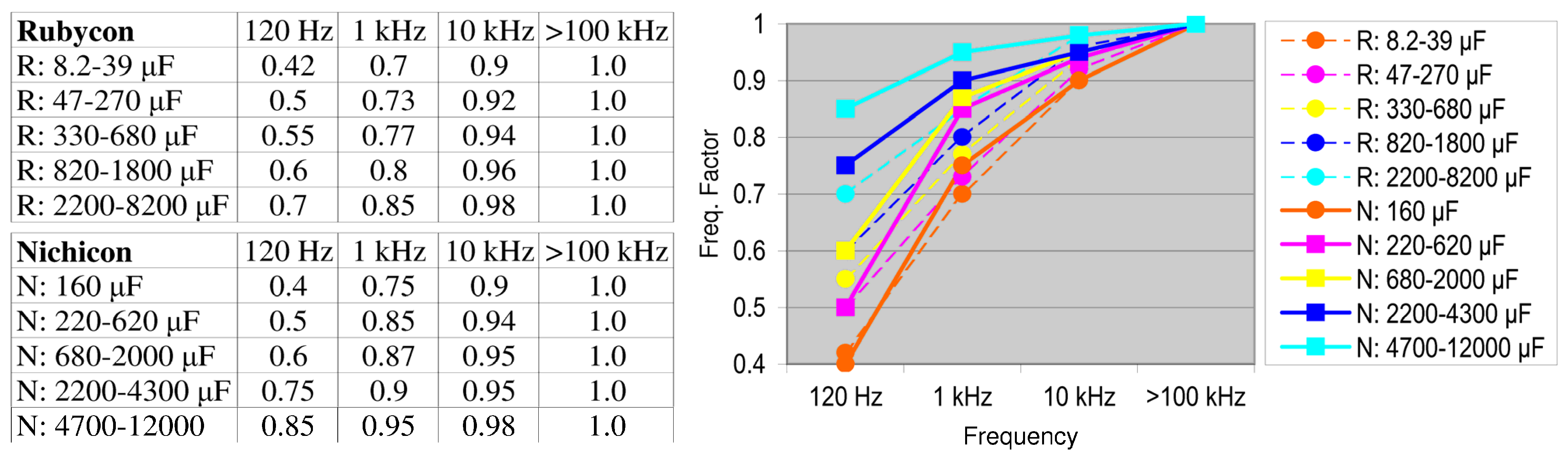
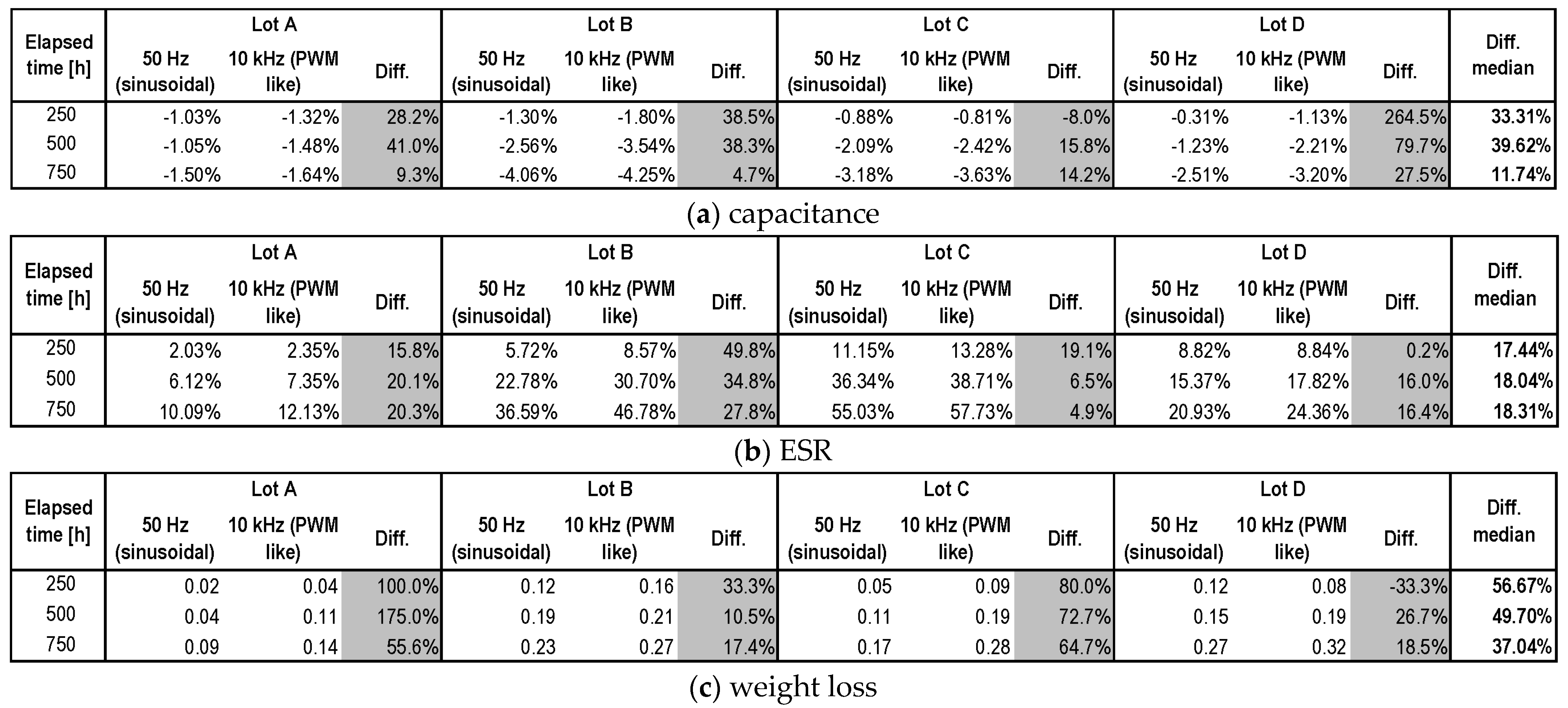
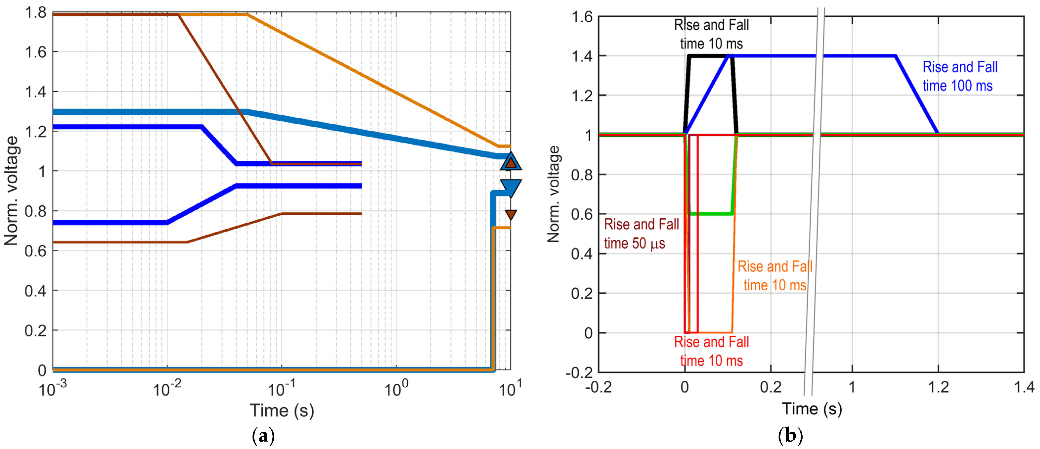
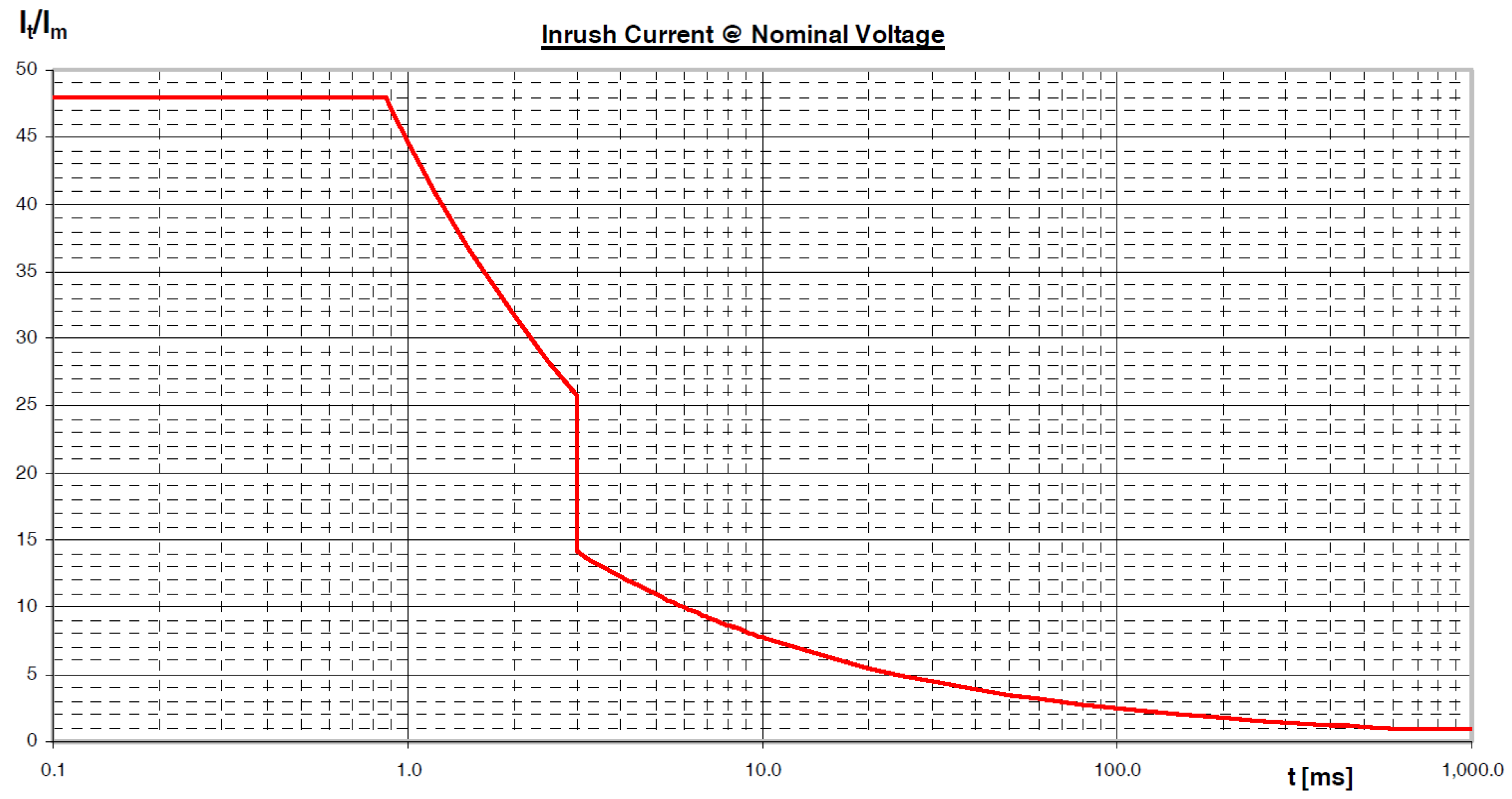
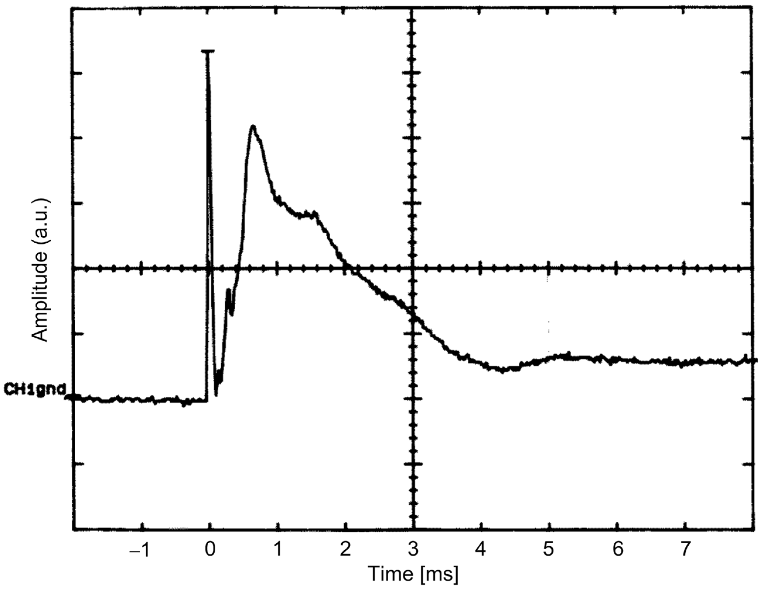
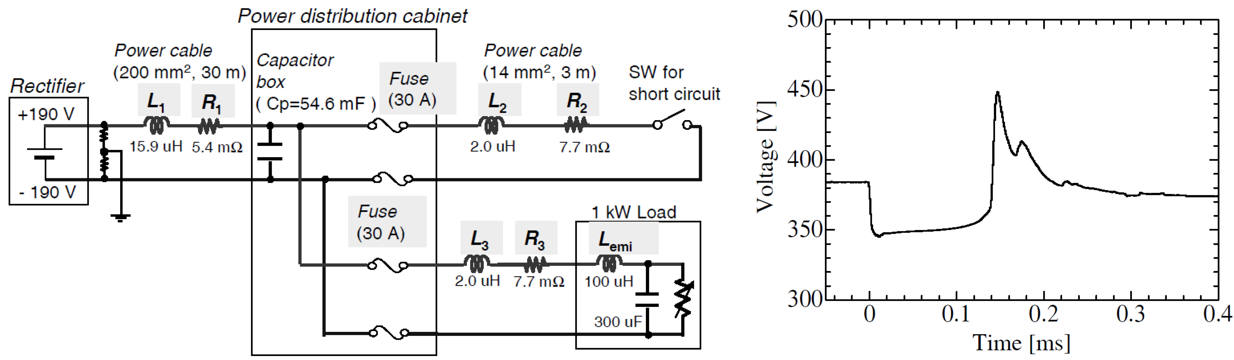
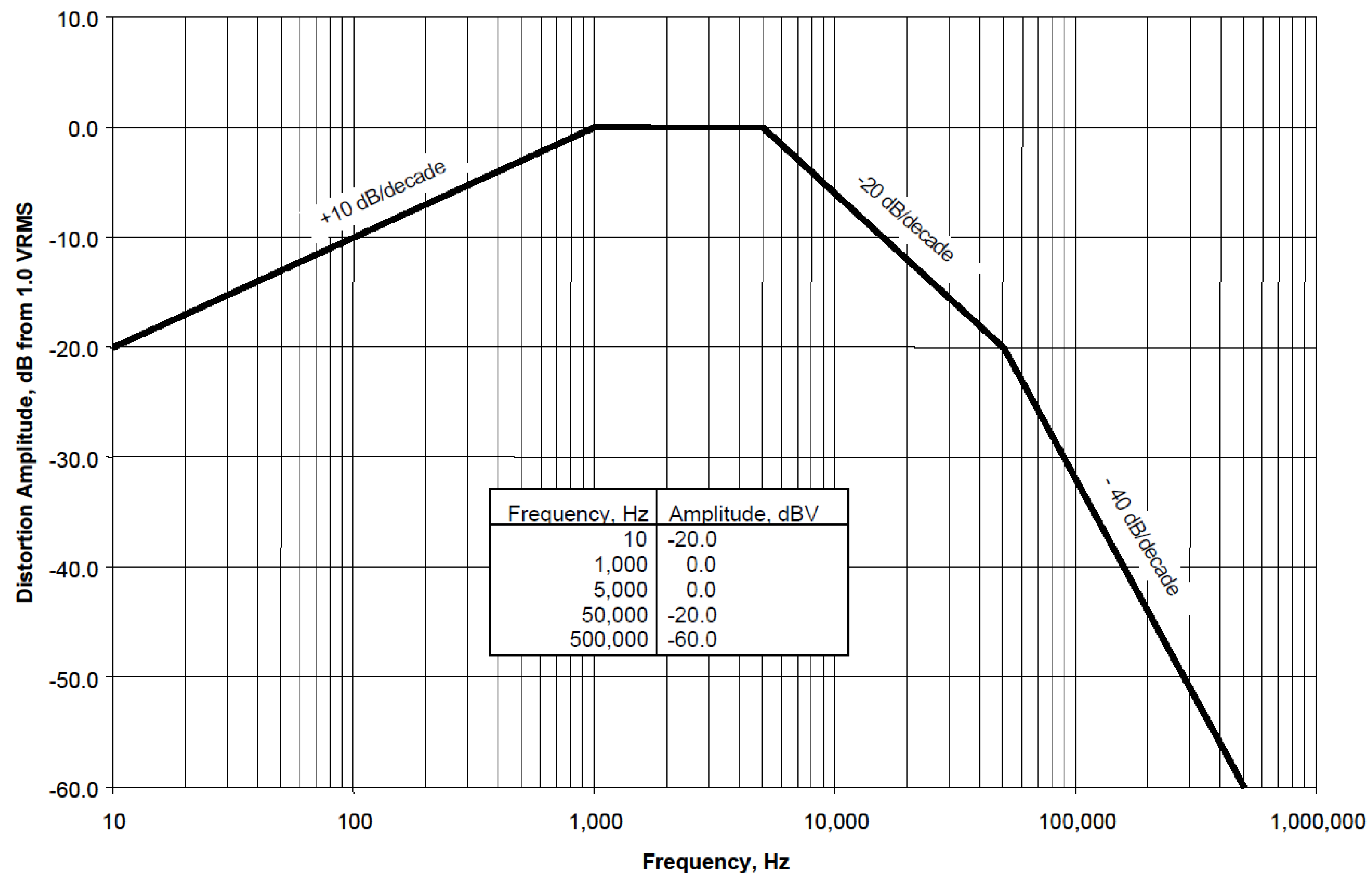
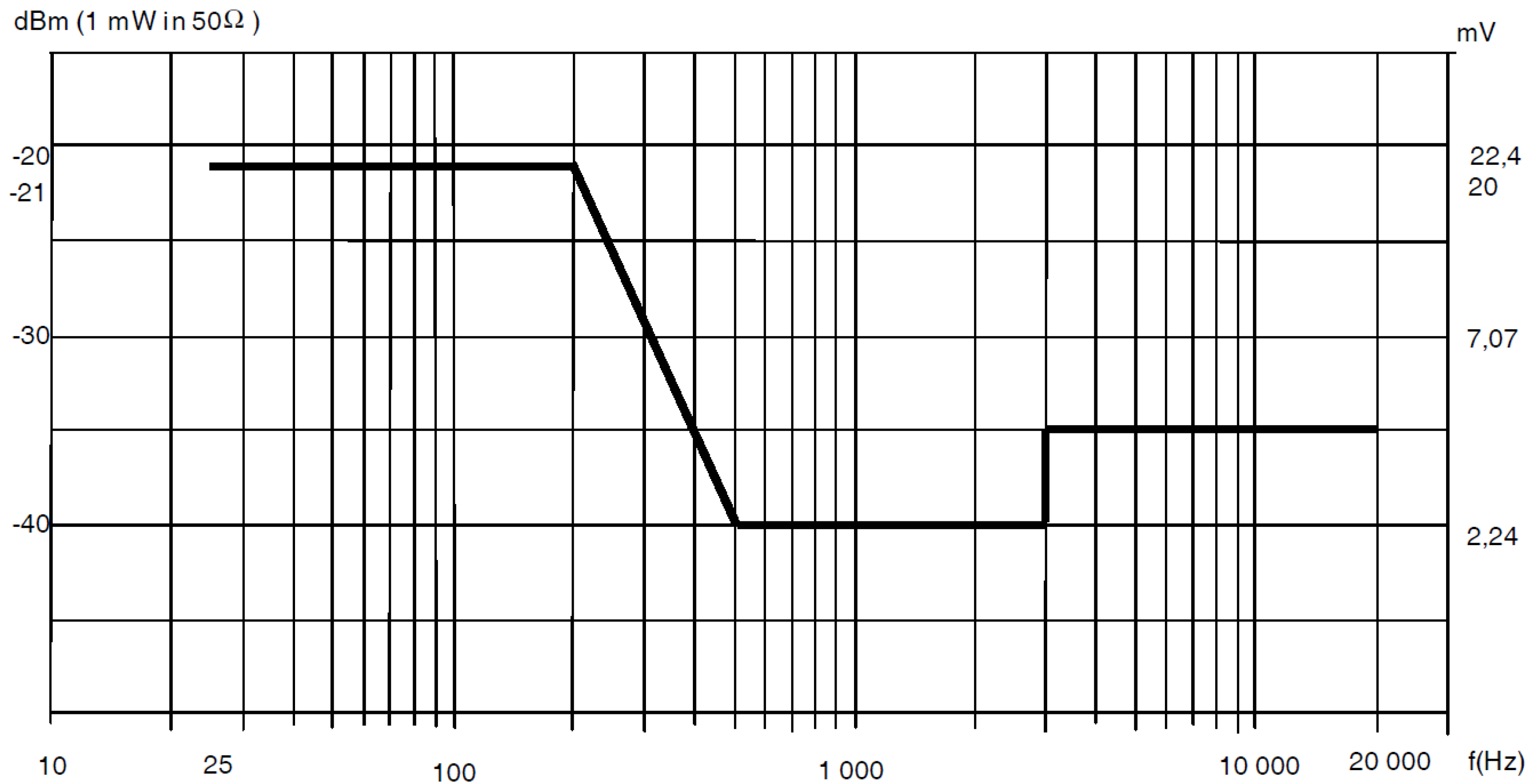
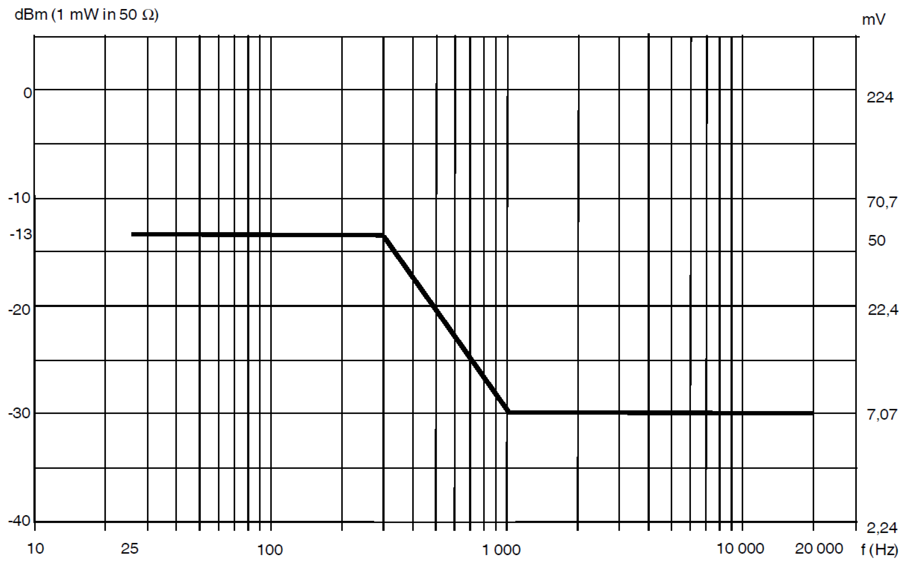
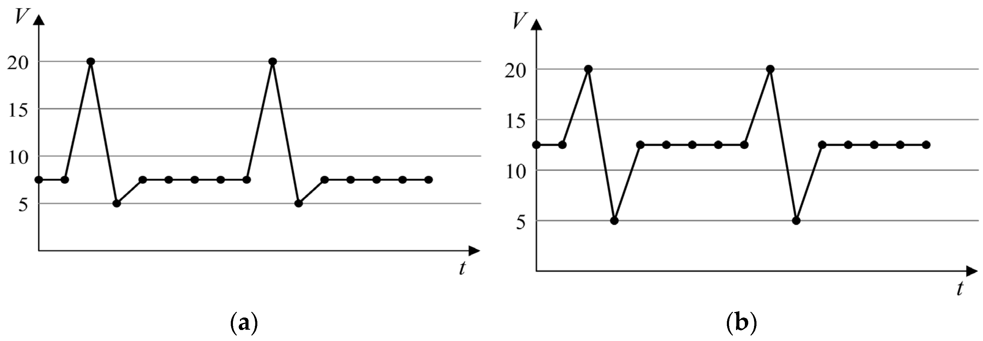
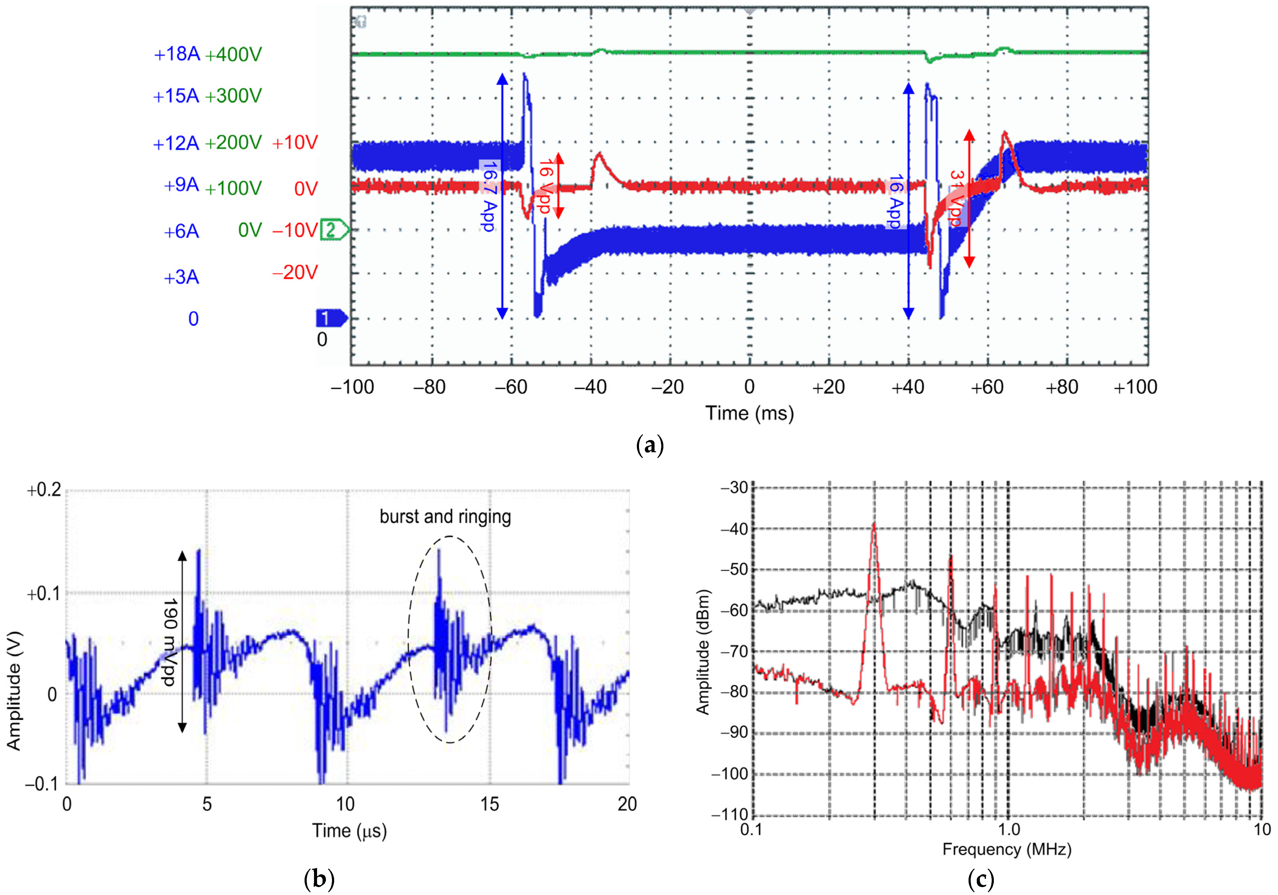
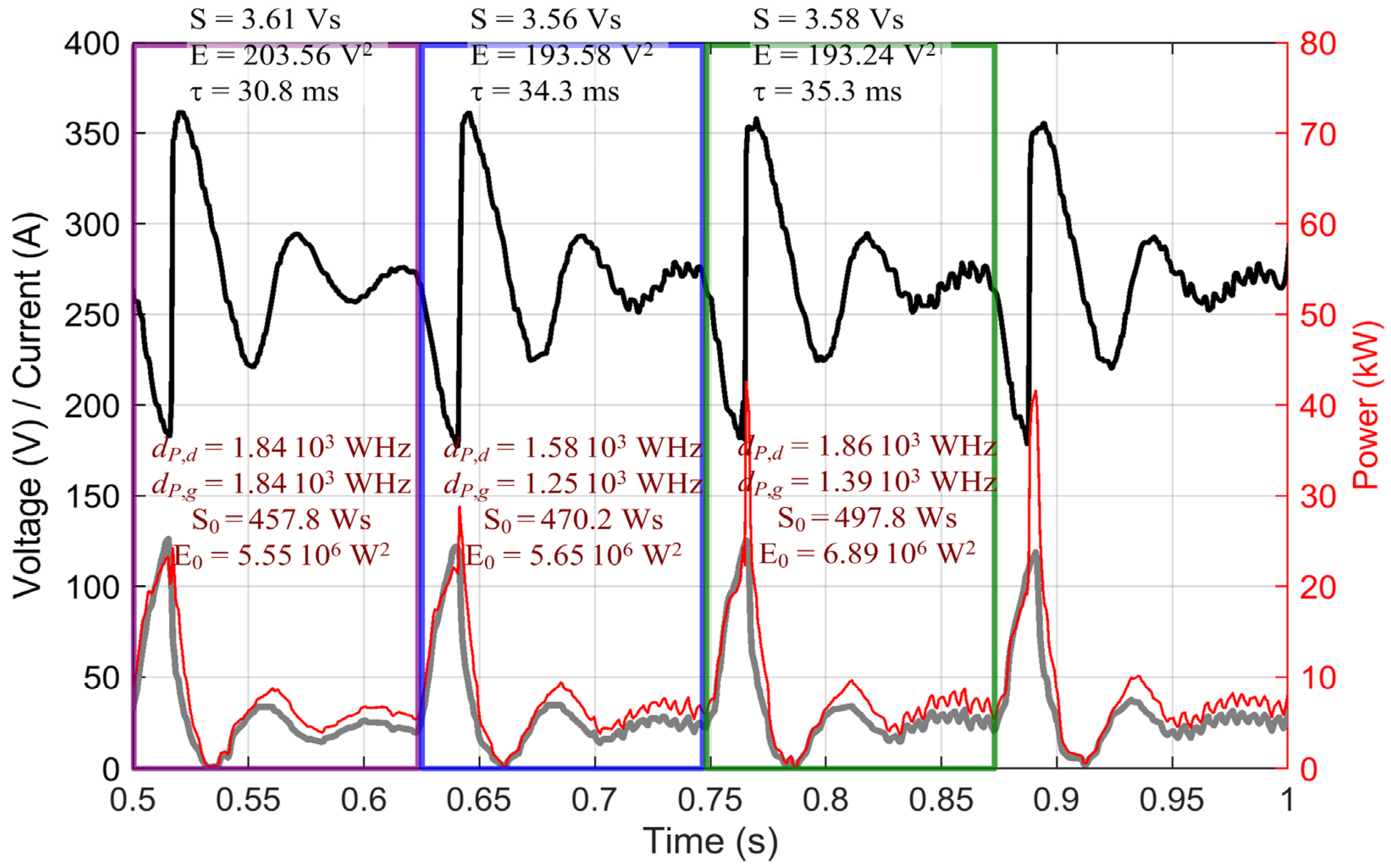
Table 1.
Summary of effect of sources and loads (and their number) on DC microgrid main resonance [29].
Table 1.
Summary of effect of sources and loads (and their number) on DC microgrid main resonance [29].
| Sources and Loads (1) (Increase Number or Rated Power) | Grid Parameters | ||||
|---|---|---|---|---|---|
| Stability (2) | Impedance | Main Res. Freq. | Main Res. Damping | ||
| Sources | Voltage controlled (VCS) | ↑ | ↓ | ↑↑ | ↑↑ |
| Current controlled (CCS) | ↓ | ↑ | ↓ | ↓↓ | |
| Loads | Constant current (CCL) | ↑ | — | ↑↑ | ↑↑ |
| Constant impedance (CIL) | ↑ | — | ↑↑ | ↑↑ | |
| Constant power (CPL) (3) | ↓ | — | ↓ | ↓↓ | |
Notes: (1) Effect of sources and loads is evaluated assuming that their number or their rated power increase; (2) Contribution to stability is neutrally evaluated, as a consequence of damping; (3) CPLs in their operating bandwidth behave like negative CILs.
Table 2.
Supercapacitors: dependency of ESR and capacitance on frequency, ripple, and number of cycles.
Table 2.
Supercapacitors: dependency of ESR and capacitance on frequency, ripple, and number of cycles.
| Ripple | ESR | Capacitance | Ref. |
|---|---|---|---|
| 20% rms, 0.1 Hz (±5 Apk sin. on 30 Adc) | linear +50% at 0–60% ripple | −5% at ≥20% ripple | Sarr * et al. [33] |
| 10% rms, 100 and 10 kHz (12 Arms sin. on 120 Adc) | +2/+20% at 1000 h, +25/+70% at 5000 h | −10/−16% at 1000 h, −25/−30% at 5000 h | German et al. [34] |
| 16.7% p-p (9.6% rms), 0.1–0.5 Hz (±5 Apk triang. on 30 Adc) | 0% at 0.2 Hz, +15% at 0.5 Hz +8% at 1000 cy (110 h), +8% at 8000 cy (900 h), +12% at 14,000 cy (1550 h) | −2% at 0.2 Hz, −3% at 0.5 Hz −2% at 1000 cy (110 h), −5% at 8000 cy (900 h), −6% at 14,000 cy (1550 h) | Bellache et al. [89] |
* Sarr et al. mix ripple and number of cycles: the longer the test, the higher the ripple, which increases by 20% every 56 h (250 cycles of 400 s duration each).
Table 3.
PV panel efficiency as a function of ripple (frequency and peak-peak amplitude) [102].
Table 3.
PV panel efficiency as a function of ripple (frequency and peak-peak amplitude) [102].
| Efficiency % | Ripple Amplitude (mA) | Ripple Frequency (kHz) | ||
|---|---|---|---|---|
| 5 | 10 | 25 | ||
| Low insolation 0.07 kW/m2 IPV,sc = 175 mA | 50 | >99 | >99 | 98 |
| 100 | 98.5 | 96 | 91.5 | |
| 150 | 97 | 87 | 74 | |
| High insolation 0.193 kW/m2 IPV,sc = 483 mA | 100 | >99 | 99 | 98 |
| 200 | 99 | 94 | 92 | |
| 400 | — | 81 | 75 | |
Table 4.
Fuel cell efficiency * as a function of ripple (frequency and peak–peak amplitude, expressed by ripple factor Ipp/Iavg) [105].
Table 4.
Fuel cell efficiency * as a function of ripple (frequency and peak–peak amplitude, expressed by ripple factor Ipp/Iavg) [105].
| Test Type | Operating Point % | Ripple Factor % | Ripple Frequency (kHz) | |||
|---|---|---|---|---|---|---|
| 30 | 60 | 120 | 1250 | |||
| Hydrogen concentration | ≤80 | >99 | >99 | >99 | >99 | |
| 98 | 91 | 96 | — | — | ||
| Oxygen concentration | 25 | 3 | >99 | >99 | >99 | >99 |
| 9 | >99 | >99 | >99 | >99 | ||
| 30 | 97 | 98.5 | 99 | >99 | ||
| 62 | 3 | >99 | >99 | >99 | >99 | |
| 9 | 98 | 99 | 99 | >99 | ||
| 30 | 93 | 95 | 96.5 | 99 | ||
| 98 | 3 | 99 | >99 | >99 | >99 | |
| 9 | 95 | 97.5 | 98 | >99 | ||
| 30 | 85 | 87 | 91 | 97.5 | ||
* Efficiency corresponds to percentage of utilization, measured as concentration of hydrogen and oxygen at electrodes.
Table 5.
Limits and test values for transient phenomena (voltage swells, sags, and interruptions) (E = emission, I = immunity, G = generator, A = ambient specification).
Table 5.
Limits and test values for transient phenomena (voltage swells, sags, and interruptions) (E = emission, I = immunity, G = generator, A = ambient specification).
| Standard | Phenomenon | Type | Nom. Volt. Un [V] | Ref. Values | |
|---|---|---|---|---|---|
| MIL-STD-704F | Voltage var. | A | 28, 270 | see Figure 3a | |
| EN 61000-4-29 | Voltage var. | I | 24–110 | 85–120%, 0.1–10 s | |
| EN 61000-4-29 | Voltage dip | I | 24–110 | 40, 70%, 0.01–1 s | |
| EN 61000-4-29 | Voltage interr. HiZ and LoZ | I | 24–110 | 0%, 0.001–1 s | |
| IACS | Voltage var. | I | ≤1kV | 95–105% | |
| Lloyd Reg. | Voltage var. | I | LV & MV | 90–110% | |
| EN 50155 | Voltage var. | I | 24–110 | see Figure 3b | |
| EN 50155 | Voltage interr. | I | 24–110 | 0%, 0.01–0.03 s | |
| L.1200 | Voltage var. | A | 300, 380 | Un→400→Un, 1 min Un→260→Un, 1 min Un→410→Un, 1 s Un→420→Un, 10 ms | |
| L.1200 | Voltage dip | I | 300, 380 | 40%, 0.01 s | |
| L.1200 | Voltage interr. HiZ & LoZ | I | 300, 380 | 0%: 0.01 s (LoZ), 1 s (HiZ) | |
Table 6.
Limits and reference values for ripple (voltage ripple, if not otherwise specified) (E = emission, I = immunity, G = generator, A = ambient specification).
Table 6.
Limits and reference values for ripple (voltage ripple, if not otherwise specified) (E = emission, I = immunity, G = generator, A = ambient specification).
| Standard | Type | Nom. Volt. Un (V) | Ref. Values | |
|---|---|---|---|---|
| MIL-STD-704F | A | 28 | DF < 3.5%; Rp,1 < 1.5/28 V | |
| MIL-STD-704F | A | 270 | DF < 1.5%; Rp,1 < 6/270 V | |
| EN 61000-4-17 | G | ≤360 V | Vrip-gen = Rpp = 2, 5, 10, 15% | |
| IACS | I | ≤1 kV | Rrms < 10% (1) | |
| EN 50155 | I | 24–110 | Rp,2, Rp,3 < 5% | |
| IEEE Std. 1662 | I | LV & MV (2) | Rrms < 10% (1) | |
| IEC 61851-23 (3) | A,E | LV | Rp,1 < 5 V | |
| Lloyd Reg. | I | LV & MV | Rrms < 10% (1) | |
Notes: (1) accompanied by specification of “voltage cyclic variation” of 5%; (2) for MV reference to IEEE Std. 1709, that covers 1 to 35 kV DC; (3) ripple specified for the charger–vehicle interface during pre-charge and charging.
Publisher’s Note: MDPI stays neutral with regard to jurisdictional claims in published maps and institutional affiliations. |
© 2021 by the author. Licensee MDPI, Basel, Switzerland. This article is an open access article distributed under the terms and conditions of the Creative Commons Attribution (CC BY) license (https://creativecommons.org/licenses/by/4.0/).
Share and Cite
MDPI and ACS Style
Mariscotti, A. Power Quality Phenomena, Standards, and Proposed Metrics for DC Grids. Energies 2021, 14, 6453. https://doi.org/10.3390/en14206453
AMA Style
Mariscotti A. Power Quality Phenomena, Standards, and Proposed Metrics for DC Grids. Energies. 2021; 14(20):6453. https://doi.org/10.3390/en14206453
Chicago/Turabian StyleMariscotti, Andrea. 2021. "Power Quality Phenomena, Standards, and Proposed Metrics for DC Grids" Energies 14, no. 20: 6453. https://doi.org/10.3390/en14206453
Note that from the first issue of 2016, this journal uses article numbers instead of page numbers. See further details here.