Load Profile-Based Residential Customer Segmentation for Analyzing Customer Preferred Time-of-Use (TOU) Tariffs

Abstract

Smart meters and dynamic pricing are key factors in implementing a smart grid. Dynamic pricing is one of the demand-side management methods that can shift demand from on-peak to off-peak. Furthermore, dynamic pricing can help utilities reduce the investment cost of a power system by charging different prices at different times according to system load profile. On the other hand, a dynamic pricing strategy that can satisfy residential customers is required from the customer’s perspective. Residential load profiles can be used to comprehend residential customers’ preferences for electricity tariffs. In this study, in order to analyze the preference for time-of-use (TOU) rates of Korean residential customers through residential electricity consumption data, a representative load profile for each customer can be found by utilizing the hourly consumption of median. In the feature extraction stage, six features that can explain the customer’s daily usage patterns are extracted from the representative load profile. Korean residential load profiles are clustered into four groups using a Gaussian mixture model (GMM) with Bayesian information criterion (BIC), which helps find the optimal number of groups, in the clustering stage. Furthermore, a choice experiment (CE) is performed to identify Korean residential customers’ preferences for TOU with selected attributes. A mixed logit model with a Bayesian approach is used to estimate each group’s customer preference for attributes of a time-of-use (TOU) tariff. Finally, a TOU tariff for each group’s load profile is recommended using the estimated part-worth.

1. Introduction

In recent years, global warming resulting from extensive carbon dioxide emissions has become an increasing concern. Accordingly, many countries have sought to establish a truly global coalition for carbon neutrality by 2050. Many countries use energy storage systems and variable renewable energy sources on the supply side and demand response, such as dynamic pricing programs, to transition from the current centralized system to a carbon-free decentralized system [1,2].

Dynamic pricing based on smart meters plays an important role in implementing a smart grid. Dynamic pricing is one of demand-side management methods that can reduce the on-peak demand by charging different prices at different times according to demand. TOU based demand-side management is proposed in [3]. Furthermore, dynamic pricing can help utilities reduce investment cost of a power system by shifting peak loads from peak to off-peak hours. Dynamic pricing contracts are available in many countries. In the United States, the most popular dynamic pricing schemes are the time-of-use (TOU) and critical peak pricing (CPP). In European countries, TOU is the most dynamic pricing scheme [4,5].

Several previous studies have analyzed how to implement an effective TOU tariff structure [6,7]. Based on these theoretical analyses, several field experiments have been implemented to evaluate the effect of dynamic pricing. The empirical results of the field experiments show that TOU or dynamic pricing decreases the peak-time electricity demand [8,9]. However, even if TOU is effective, it is unclear whether customers prefer TOU instead of existing flat pricing. Additionally, if customers prefer the TOU tariff, then which attribute of the TOU tariff is preferred. In estimating the preference of virtual goods, the application of a discrete choice model such as a choice experiment is increasing. A choice experiment has the advantage of being able to estimate customers’ the benefits of various changes according to the preference estimation for each attribute. Therefore, to investigate customer acceptance of the TOU tariff and its most preferred attributes by customers, a choice experiment is conducted.

Several previous studies have used the choice experiment presented in this study. Ozbafli and Jenkins studied 350 households in North Cyprus using a choice experiment. While this study did not estimate the preference for electricity tariffs, it estimated the willingness to pay (WTP) of customers for reliable electricity supply [10]. Christian et al. analyzed strong customer preference for prevailing time-invariant pricing plans compared with time-variant pricing plans for electricity services. They compared customer preferences for different pricing plans using a modification of the traditional discrete choice experiment. They found that households rejected dynamic pricing due to unpredictable price variations [11]. Elisabeth et al. investigated the type of pricing preferred and why, based on the following two empirical studies from Germany. First was a questionnaire study including a choice experiment, and the second was a field experiment with test residents of a smart-home laboratory. They found that customers interested to dynamic pricing but preferred simple programs to complex and highly dynamic ones. A limitation of this study is that the experimental environment is not real, and the attributes constituting the choice experiment are not representative of the dynamic pricing plan. [12]. Yoshida et al. investigated customers’ preferences for dynamic pricing by studying customers living in Japan using a choice experiment. Yoshida et al. found that TOU was the preferable pricing method for customers, and TOU had the highest value of willingness to pay (WTP) among other dynamic pricing schemes. Their investigation results show that household characteristics are important factors in the choice of dynamic pricing. However, Yoshida et al. only used a conditional logit model that is not fully reflected the preferences for dynamic pricing of each customer [13]. Most recently, in Germany, consumers’ acceptance of TOU tariffs was analyzed using a choice experiment. It showed that about 70% of respondents chose a TOU tariff. The limitation of the study conducted in Germany was that the number of attributes constituting the choice experiment survey was small, and the attributes consisting of the TOU tariff were not sufficiently considered [14].

CE in the previous studies only aimed to investigate the customers’ preferences for TOU tariff with other pricing program. For example, dynamic pricing program of attributes are also fixed by researchers, and customers’ preferences are estimated between different dynamic pricing programs. Therefore, research on which TOU tariff attributes are important to customers is lacking. Furthermore, little is known about customer preferences for TOU tariff plans and attributes based on the daily load profile of the customer. However, it is important to consider the load profiles when analyzing the preferences for TOU tariffs. For example, when choosing a TOU tariff plan, customers can consider their daily electricity usage patterns over time. This is because customers do not have the opportunity to reduce their electricity usage and generally do not want longer peak time periods when they use little electricity during peak time periods. To the best of knowledge, this study is the first attempt to analyze customer preferences for TOU tariff plans and attributes based on the customer’s daily load profile. Therefore, in this study, customers were clustered according to their load profiles. Subsequently, each group’s attribute preferences of the TOU tariff are investigated using the choice experiment. Lastly, the most preferred TOU tariff design is presented in an enumeration method based on each group’s preferred attribute.

The remainder of this paper is organized as follows: Section 2 describes the method used to cluster the residential load profile. Section 3 introduces the method for the choice experiment to identify customers’ preferences for TOU tariffs. Section 4 presents the results of the analysis using the method proposed in this study. Finally, Section 5 concludes the paper.

2. Clustering Method for Residential Load Profiles

2.1. Feature Definition for Clustering Residential Load Profiles

In this study, in order to analyze which TOU tariff plan is preferred based on the daily usage patterns of residential customers, the load profiles of each residential customer are obtained using the median value for each hour to construct a representative load profile. This is done to cluster thousands of customer load profiles into the number of consumption patterns that can be analyzed. The median value is used because it is less affected by anomalous data than the average value. A representative load profile is normalized by the hour using the min-max normalization method to compare patterns for each customer. The load profiles of each customer are normalized as follows [15]:

$$Loa{d}_{i,h}^R=median\left(z\right), where z\in Loa{d}_j,j\in {\theta }_h$$

(1)

$$Normalized\_L_{i,h}=\frac{L_{i,h}-min\left(L_i\right)}{max\left(L_i\right)-min\left(L_i\right)}$$

(2)

where, $Loa{d}_{i,h}^R$ is the representative load at hour h for customer i. ${\theta }_h$ is the set of previous h hours on the same day. z is the electricity consumption during ${\theta }_h$. $Normalized\_L_{i,h}$ is the normalized electricity consumption of customer i at time h. $L_{i,h}$ is the median electricity consumption of customer i at time h. $L_i$ is the load profile of customer i.

As a person’s behavior can be characterized during specific time intervals (for example, commuting or working), it is essential to understand the behavioral patterns of customers over time. Considering that the first bus time in Korea is usually 5:00 AM, the morning period is assumed to start at 4:00 AM in this study. Because some non-working family members have morning routines, such as watching TV, doing laundry, and vacuuming, the morning period is assumed to end at 11:00 AM. It can be observed from Figure 1 that the electricity usage pattern increases from around 4:00 AM, peaks at 8:00 AM, and shows a constant usage pattern after 11:00 AM. Since working hours end around 18:00 PM in Korea, the daytime period is assumed to end at 18:00 PM. The electricity usage pattern drops sharply after 22:00 PM so that the evening period is assumed to end at 22:00 PM in this study. Therefore, the time periods are classified as morning, daytime, evening, and night. The four time periods are as follows:

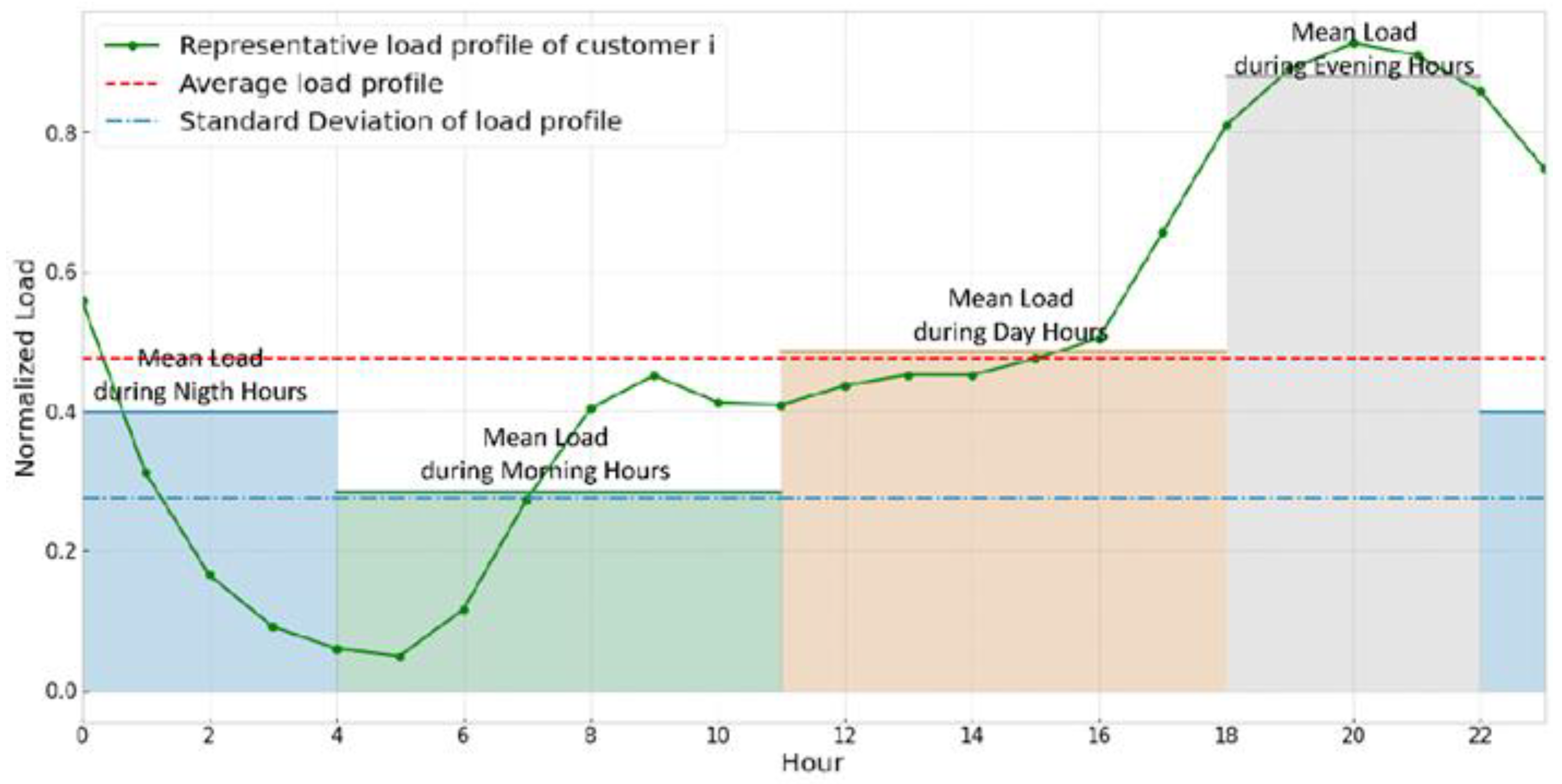
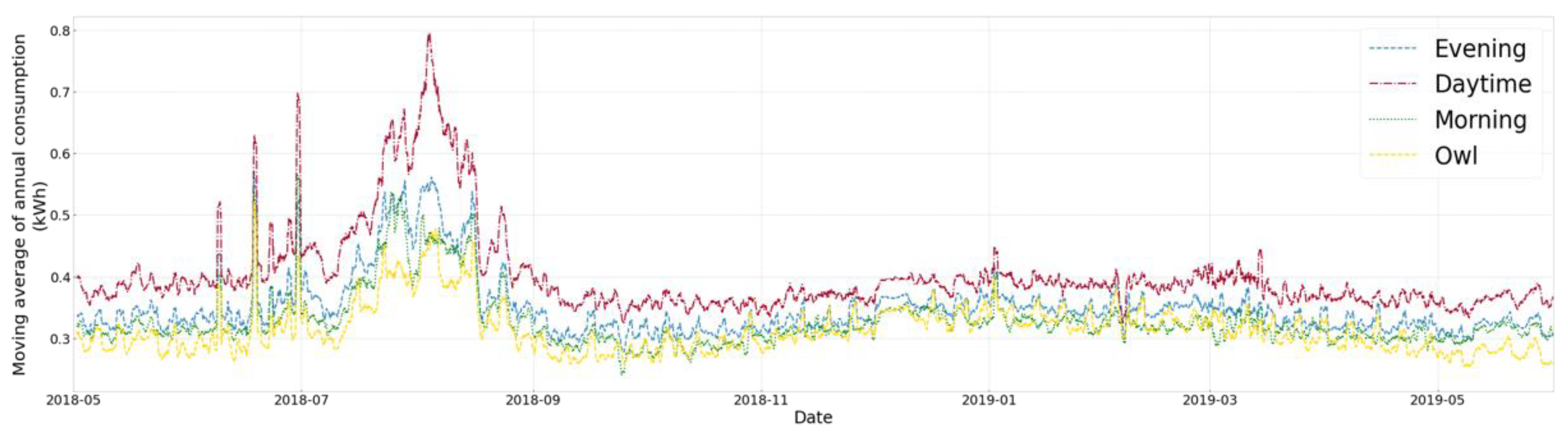
• Night period: 22:00 PM–04:00 AM
• Morning period: 04:00 AM–11:00 AM
• Daytime period: 11:00 AM–18:00 PM
• Evening period: 18:00 PM–22:00 PM

Furthermore, some residential customers use electricity throughout the day because of unemployed older adults, elementary school students, or preschool children. If the average normalized load profile is close to the average of the daytime period, the customer is more likely to use electricity during the daytime period. In addition, if the standard deviation of the normalized load profile is relatively small, the electricity consumption of a residential house can be considered to remain constant. Therefore, the standard deviation and average of customers’ electricity use patterns are defined. Figure 2 shows an example of the normalized daily load profile of a residential customer, and six features are defined for clustering the load profiles as follows:

$$AvgLoa{d}_i={\displaystyle \sum _h}N\_Loa{d}_{h,i}/ 24 where h\in \left(0,23\right)$$

(3)

$$StdLoa{d}_i=\sigma (N\_Loa{d}_{h,i})$$

(4)

$$\frac{{\sum }_{h}N\_Loa{d}_{h,i}}{p}\{\begin{array}{c}AvgMornin{g}_i, if p\in morning period\\ AvgDytim{e}_i, if p\in daytime period\\ AvgEvenin{g}_i, if p\in evening period\\ AvgNigh{t}_i, if p\in night period\end{array} where h\in p$$

(5)

where, $N\_Loa{d}_{h,i}$ is the normalized load of customer i at time h. $AvgLoa{d}_i$ is the average normalized load of customer i. $StdLoa{d}_i$ is the standard deviation of the normalized load of customer i. $AvgMornin{g}_i$, $AvgDaytim{e}_i$, $AvgEvenin{g}_i$ and $AvgNigh{t}_i$ are the average of the normalized load in each period defined in this study.

Six features, which are defined in Equations (3)–(5), extracted from the normalized load profiles of all customers. Therefore, the daily load profile of customer i can be defined by six features in Equation (6). Six features are utilized to group residential customers into K clusters using GMM:

$${\mathrm{C}}_{\mathrm{i}}=\left\{{\mathrm{AvgLoad}}_{\mathrm{i}}, {\mathrm{StdLoad}}_{\mathrm{i}}, {\mathrm{AvgMorning}}_{\mathrm{i}}, {\mathrm{AvgDaytime}}_{\mathrm{i}}, {\mathrm{AvgEvening}}_{\mathrm{i}}, {\mathrm{AvgNight}}_{\mathrm{i}}\right\}$$

(6)

2.2. Gaussian Mixture Model (GMM) for Clustering Residential Load Profiles

The Gaussian Mixture Model (GMM) is s a parametric probability density function representing a dataset with a weighted sum of several normal distributions called mixture components [16]. The GMM can be described as follows [17]:

$$p(X|{\mu }_k,{\displaystyle \sum _k},{\omega }_k)={\displaystyle \sum _{k=1}^K}{\alpha }_k{\omega }_k(X|{\mu }_k,{\displaystyle \sum _k})$$

(7)

$${\omega }_k(X|{\mu }_k,{\displaystyle \sum _k})=\frac{1}{{\left(2\pi \right)}^{\frac{d}{2}}{\left|{\sum }_k\right|}^{\frac{1}{2}}}\exp \{-\frac{1}{2}{\left(X-{\mu }_k\right)}^T{\displaystyle \sum _k}{}^{-1}\left(X-{\mu }_k\right)\}$$

(8)

where $\omega$ is the Gaussian probability density function. K is the number of mixture models. ${\alpha }_k$ is set of the mixture weights. ${\mu }_k$ and ${\sum }_k$ indicate the mean vector and covariance matrix. Each Gaussian model represents a cluster [18]. X is the feature set defined in Equation (6)

The expectation maximization (EM) algorithm is commonly used to estimate GMM, and EM is divided into two steps: expectation and maximization [19]. In the expectation step, each observation is assigned to one of the mixture components that assigns the highest probability to this observation. Next, the parameter of each mixture component is updated in the maximization step based on the location of the observations assigned to the mixture component. After an initial set of the model parameters is first randomly selected, the expectation and maximization steps are iteratively computed until likelihood function in Equation (9) is convergence [20]:

$$lnp(X|{\mu }_k,{\displaystyle \sum _k},{\omega }_k)={\displaystyle \sum _{i=1}^N}\ln \{{\displaystyle \sum _{k=1}^K}{\alpha }_k{\omega }_k\left(X|{\mu }_k,{\displaystyle \sum _k}\right)\}$$

(9)

where N is the number of samples, $lnp(X|{\mu }_k,{\sum }_k,{\omega }_k)$ is the natural log of Equation (7). $\omega$, ${\alpha }_k$, ${\mu }_k$, ${\sum }_k$, and X are the same as those in Equation (7). A key problem in GMM-based clustering is to determine the optimal number of components, K. The Bayesian information criterion (BIC), one of the most widely used criterion for statistical model selection, is used to select the number of components, as follows [21]:

$$BIC=-L(X|{\mu }_k,{\sum }_k,{\omega }_k)+\frac{W}{2}\log \left(N\right)$$

(10)

$$W=Kd+\frac{1}{2}Kd\left(d+1\right)+\left(K-1\right)$$

(11)

where, $L(X|{\mu }_k,{\sum }_k,{\omega }_k)$ is log likelihood function defined in Equation (9), W is the total number of estimated parameters, N is the number of sample and d is set to 6 in this study.

3. Choice Experiment for Customers’ Preference for Time-of-Use (TOU) Tariff

3.1. Design of the Choice Experiment

A choice experiment is a multivariate analysis that identifies respondents’ preferences for virtual products or services that consist of the selected attributes. This method identifies respondents’ preferences through the levels that make up each attribute of virtual services and analyzes the importance of each attribute that customers consider [22,23].

The following should be considered to identify customer preferences accurately through choice experiments: First, it is recommended that the number of attributes is eight or fewer, and each attribute must be independent of each other [23]. However, each attribute can be divided into several levels. Second, the choice experiment separates the influence of individual attributes on the selection behavior. Therefore, it uses the main effects orthogonal design method that ensures orthogonality between individual properties. The orthogonal design method solves the problem of choice experiments owing to the high correlation between attributes [24]. Finally, a discrete selection model is used to analyze consumers’ preference data.

To describe the TOU tariff, several attributes were selected as follows: rate design, month, weekends, and peak-times.

Table 1. Attributes and levels of TOU tariff in the choice experiment survey.

Attributes	Levels
Rate design		Structure	Off-peak rate 1	Mid-peak rate 1	On-peak rate 1	On-to-off peak rate ratio
	Rate A	2	82	-	188	2.3
	Rate B	2	77	-	246.4	3.2
	Rate C	2	73	-	316	4.2
	Rate D	3	82	155	188	2.3
	Rate E	3	77	155	246.4	3.2
	Rate F	3	73	155	316	4.2
Month	2 month(July-August)/3 month(June-August)/4 month(May-August)
Weekends	only weekdays/all week
Peak-times	2 h per day/3 h per day/4 h per day

Note: ¹ US$1 = 1165.00 KRW (at August 2021).

presents the levels of each attribute according to the TOU tariff for choice experiment survey. There are some descriptions about Weekends attribute. If a customer chooses TOU tariff applied all week, off-peak rate (73 KRW/kWh) and on-peak rate (188 KRW/kWh) apply on weekends. On the other hand, if customers choose TOU tariff that applied only on weekdays, mid-peak rate (155 KRW/kWh) and off-peak rate (82 KRW/kWh) apply on Saturday, and only off-peak rate (82 KRW/kWh) apply on Sunday.

This study analyzes consumers’ preferences for TOU tariffs according to Rate design, Month, Peak-times, and whether to apply all weeks, that is, Weekends. Designing a choice set to influence the respondents’ probability of selecting a TOU alternative is critical in choice experiments. Therefore, this study uses an orthogonal main effects design that ensures the orthogonality of each attribute to construct a simplified alternative card for the survey. Thus, this method produces four alternative choice sets consisting of four cards. The preference of each attribute is analyzed based on the respondents’ choice. The four alternative choice sets used in the study are used for choice experiment survey and the example of choice set is shown in

Table 2. Choice set example of TOU tariff in the one-to-one individual survey.

	Rate Design	Month	Weekends	Peak-Times
Type A	Rate D	July–August	Yes	4 h/day
Type B	Rate E	July–August	No	3 h/day
Type C	Rate A	July–August	Yes	3 h/day
Type D	Rate F	May–August	No	2 h/day

.

3.2. The Mixed Logit Model for Analyzing the Choice Experiment

The conditional logit model is easy to estimate and interpret the results. However, it is difficult to explain the heterogeneity in preferences among individual consumers fully. This study considers preference heterogeneity for each customer using a mixed logit model. TOU tariff attributes preferred by consumers differ according to the environment for electricity consumers. Preferred heterogeneity is divided into two categories: systematic preference heterogeneity, representing observed characteristics, and heterogeneity, indicating unobserved characteristics [25]. The mixed model estimates the distribution of coefficients representing the effects of attributes reflecting preferences for the TOU tariff. This model can also account for the heterogeneity in which individual consumers have different preferences for different factors. Residential consumer preferences consist of two parts of the proposed questionnaire: deterministic parts related to the observed characteristics and stochastic parts related to uncertainty. If respondent n encounters the selection T sets with J alternatives, the utility of respondent n for alternative j in the selection t set is as follows:

$$U_{njt}={\beta }_n{x}_{njt}+{\epsilon }_{njt}$$

(12)

where,$x_{nj\mathrm{t}}$ is a vector of attributes that associated with respondent n and alternative $j$ in selection situation $t$ and ${\beta }_n$ is a vector of coefficients associated with each attribute. ${\epsilon }_{nj}$ is assumed to be a random variable and indicates a distribution similar to the extreme type I distribution. The coefficient vector ${\beta }_n$ assumes that the parameter $\theta$ is a probability density function that follows a normal or lognormal distribution, that is, $f\left(\beta |\theta \right)$. The probability $P_{njt}\left(\beta \right)$ of a respondent n choosing an alternative j in situation t for a given ${\beta }_n$ is estimated by a mixed-logit model in this study.

As $P_{njt}\left(\beta \right)$ cannot have the closed form solution, it is estimated as a simulation for parameter estimation. The approximate value ($\acute{P_{njt}})$ is calculated by obtaining $\beta$ values as many as R from $f\left(\beta |\theta \right)$:

$$\acute{P_{njt}}=\frac{1}{R}{\displaystyle \sum _{r=1}^R}\frac{exp\left({\beta }_r{x}_{njt}\right)}{{\sum }_{k=1}^{J}exp\left({\beta }_r{x}_{nkt}\right)}$$

(13)

The Bayesian method with Gibbs sampling is adopted to estimate the mixed logit model in Equation (13). Bayesian estimation is better than the maximum likelihood estimation (MLE) method and has more advantages [25,26].

Lastly, the relative importance of each attribute, related to decision-making, might be different in customers’ selection of alternatives. The relative importance of each attribute m can be calculated from the part-worth of each level consisting of attribute m. The range of the part-worth of attribute m is obtained from the difference between the maximum and minimum levels of attribute m [27]. The equations of relative importance are as follows:

$$Range of Partwort{h}_m=max\left({\beta }_{mk}\right)-min\left({\beta }_{mk}\right)$$

(14)

$$Relative importanc{e}_m=\frac{Range of Partwort{h}_m}{{\sum }_{m=1}Range of Partwort{h}_m}\times 100$$

(15)

4. Empirical Results

4.1. Description of Data

For accurate data collection, a one-to-one individual survey was conducted. Respondents’ demographic characteristics were surveyed to identify heterogeneity among the 529 residential customers living in apartment houses with conducting the choice experiment survey by the end of April 2021.

Table 3. Summary of residential customers in this study.

Characteristic	Index	Categorization	Number of Respondents
Family member	1	single	31
	2	two	142
	3	three	126
	4	four	169
	5	$\ge$five	61
Unemployed older adult	1	single	84
	2	$\ge$two	62
Elementary student	1	single	77
	2	$\ge$two	26
Family income	1	$\le$2.4 million ₩	103
	2	2.41–3.1 million ₩	76
	3	3.11–4.4 million ₩	102
	4	4.41–5.1 million ₩	78
	5	5.11–7.3 million ₩	100
	6	≥₩7.31 million ₩	70
House area	1	33.1–62.8 m2	52
	2	66.1–95.6 m2	99
	3	99.2–128.9 m2	250
	4	≥132.2 m2	127
Education level	1	≤middle school	31
	2	high school	148
	3	university	307
	4	graduate school	43

presents a summary of the demographic data.

4.2. Results of Clustering of Load Profiles

The electricity consumption data of 529 customers from May 2018 to May 2019 were obtained from smart meters. Features described in Section 2.1. are extracted following Equations (1) to (5). Figure 3 shows the result of the optimal cluster number from conducting cluster method described in Section 2. BIC has a minimum when the value of K is 4. The BIC continues to increase above the point of four. Therefore, the optimal cluster number K is four based on the BIC.

Figure 4. shows the clustering results, which represent a representative load profile of residential customers. In addition, to describe the annual load profile of each group, representative annual consumption is extracted using the median of hourly consumption for each group. After the annual load profile is extracted, a moving average using a 24-h window is applied to the representative annual consumption to clearly show the differences between each group. Figure 5. shows the moving average of the annual load profiles for each group. The evening pattern (258 customers) is the typical load profile of customers who use electricity for commuting to work in the morning but are not home in the afternoon and begin their evening routine after leaving the office. The daytime pattern (68 customers) shows electricity use during the day, indicating that other family members such as preschool children and unemployed older people use the appliances in the house. The morning pattern (67 customers) describes residential customer activity with a temporary increase in electricity during the morning and no electricity usage until the evening routine. The owl pattern (136 customers) shows high energy consumption during the night and may increase briefly in morning hours, and is rarely used during the day, before increasing again in the evening.

Table 4. Average of the demographic index by each group.

	Group
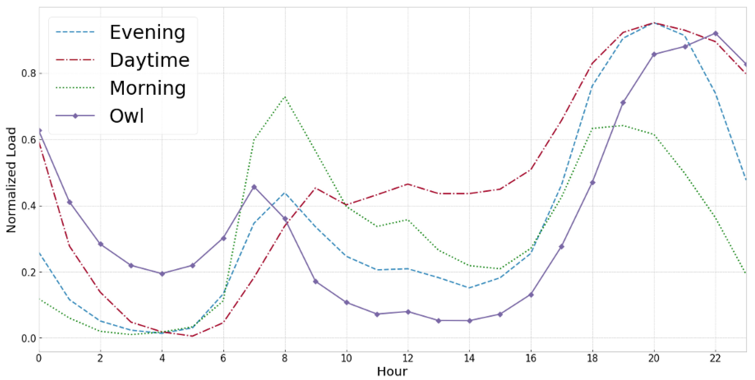
	Evening	Daytime	Morning	Owl
Family member	3.35	3.29	2.79	2.97
Unemployed older adults	1.43	1.63	1.38	1.35
Elementary student	1.25	1.36	1.00	1.28
Family income	3.54	3.42	2.9	3.29
House area	2.98	2.82	2.79	2.63
Education level	2.75	2.77	2.62	2.52

. shows the average of each group in the demographic characteristic indices that are dimensionless and defined in Table 3. The evening and daytime groups had more family members than the other groups. It may be inferred that the generally known residential load shape indicates the increased number of family members. The daytime group had relatively many unemployed older adults and elementary school children, who might increase electricity consumption during the daytime. Differences in family income and housing area are very intuitive. This is because the higher the number of family members, the higher the family income. For this reason, house area and education level have the same results.

4.3. Results of Cojoint Analysis of Each Group

A total of 25,000 draws were conducted with Gibbs sampling to estimate the mixed logit using the Bayesian method.

Table 5. Estimation of choice experiment using the mixed logit model.

	Group
	Evening	Daytime	Morning	Owl
Levels	Part-Worth
Rate B	−1.008 *** (0.109)	−0.976 *** (0.265)	−0.997 *** (0.276)	−0.797 *** (0.147)
Rate C	−0.334 *** (0.078)	−1.08 *** (0.277)	−0.259 (0.194)	−0.506 *** (0.153)
Rate D	−0.218*** (0.091)	−0.42* (0.229)	−0.224 (0.220)	−0.266 * (0.144)
Rate E	−0.276 *** (0.727)	−0.818 ** (0.267)	−0.126 (0.241)	−0.37 ** (0.18)
Rate F	−0.596 *** (0.107)	−0.417 (0.266)	−0.438 * (0.241)	−0.574 *** (0.159)
3 Months	0.053 (0.079)	−0.03 (0.230)	−0.221 (0.202)	−0.02 (0.119)
4 Months	−0.071 (0.083)	0.05 (0.27)	−0.320 * (0.198)	−0.02 (0.114)
Weekends	0.996 *** (0.079)	0.876 ** (0.249)	1.21*** (0.213)	0.724 *** (0.158)
3 h/day	−0.199 * (0.080)	0.125 (0.235)	−0.524 ** (0.234)	−0.233 * (0.143)
4 h/day	−0.125 * (0.078)	−0.0003 (0.196)	−0.362 * (0.209)	0.04 (0.143)

Note: ***, **, *; significance at 1%, 5%, and 10%, respectively. Standard error is in parentheses. Rate A, 2 Months and 2 h/day are assumed to be the base attribute.

. provides the estimated customers’ part-worth by the TOU tariff attribute and cluster using the mixed logit model explained in Section 2. The normal distribution has no restrictions. Therefore, the parameters were estimated using the normal distribution in this study.

Table 6. Relative importance of attribute by group.

	Group
	Evening	Daytime	Morning	Owl
Attributes	Relative Importance (%)
Rate design	43.31	49.96	33.77	43.93
Month	5.34	3.70	7.50	1.12
Weekends	42.80	40.55	40.98	39.91
Peak-times	8.55	5.79	17.75	15.04

Note: Relative importance is calculated with no significant coefficients in each attribute. The coefficients of base levels in each attribute are assumed to be zero.

. shows the relative importance calculated from part-worth of each group.

The results of the mixed logit model are interesting. Considering the Rate design, which has the highest relative importance, except for the morning group, shows a similar preference to Rate D relative to the base rate design, that is, Rate A. As Rate A differs from Rate D only in the structure (i.e., tier), it can be inferred that most residential customers show higher utility for on-peak rate than the tier of the TOU tariff. For the estimation result of Month, no significant coefficient was estimated in most groups except for the morning group. Additionally, the relative importance of Month is minimal. This estimation result indicates that customers have little utility in the number of months of choosing the TOU tariff. For estimation results of Weekends, the relative importance and utility of Weekends are relatively high. This may be because that if applying TOU tariff on all week is selected, then the off-peak rate is lower than applying TOU tariff only on weekdays. It is very probable that if the weekend tariff structure is designed to the customers’ preferences, it can induce the selection of the TOU tariff. Lastly, according to the Peak-times estimates, in all groups except for the daytime group, the coefficient of peak-times is significant and has a very negative value. The daytime group can respond effectively during the on-peak rate period because there is constant electricity consumption in the afternoon. However, because the electricity consumption of other groups was lower in the afternoon, they could not reduce their electricity consumption any further. Furthermore, in the morning and owl groups with fewer family members, the relative importance of Peak-times is high, and relatively high negative preference is estimated. It is reason that suppose the number of household members is small, then there is a small probability of people in the house during the peak rate period. Therefore, it can be inferred that customers with fewer family members do not prefer longer peak times.

It is reasonable to suppose that a TOU design with close part-worth to a TOU design composed of base levels in each attribute satisfies both customers and utility company. Therefore,

Table 7. TOU tariff design for each group by enumeration method.

Groups	Attributes				Total Part Worth
	Rate Design	Month	Weekends	Peak-Times
Evening	Rate D	2 Months	Yes	4 h/day	0.653
Daytime	Rate D	2 Months	Yes	2 h/day	0.456
Morning	Rate F	4 Months	Yes	4 h/day	0.09
Owl	Rate D	2 Months	Yes	3 h/day	0.225

Note: The coefficients of base levels in each attribute are assumed to be zero. Levels that are not statistically significant are excluded.

presents the TOU tariff designs for each group with the closest part-worth to the TOU tariff with base levels.

5. Conclusions

In this study, the load profiles of Korean residential electricity customers were clustered into four groups. The four groups were explained through the demographic characteristics of the customers.

Customers’ preferences for TOU tariffs in each group were analyzed with Rate design, Month, Weekends, and Peak-times, the main attributes in composing a TOU tariff. The results of the mixed-logit model with Bayesian estimation describe each customer’s preference for attributes of the TOU tariff in each group. Finally, a rate design for the load profile was suggested based on the preference for the attributes of each group.

Therefore, the TOU rate recommended for the Evening group is Rate D and 4 h/day peak times on both weekdays and weekends for 2 months. For the Daytime group, the suggested TOU rate is Rate D and 2 h/day peak times on both weekdays and weekends for 2 months. The TOU tariff plan recommended for the Morning group is Rate F and 4 h/day peak times on both weekdays and weekends for 4 months. Lastly, the TOU tariff plan suggested for the Owl group is Rate D and 3 h/day peak times on both weekdays and weekends for 2 months.

Considering residential load profiles when designing TOU tariffs for each customer could be an efficient design approach. This is because the residential electricity consumption can be measured in real-time.

Validation with customer feedback will require further TOU pilots based on each group’s preferred TOU tariff plan. The future study of the additional TOU pilots based on preferred TOU tariff plan will help analyze how the preferred TOU tariff plan influences the load shift of individual customers.

References

- Fitiwi, D.Z.; Santos, S.F.; Catalão, J.P.S. Role of Distributed Energy Storage Systems in the Quest for Carbon-Free Electric Distribution Systems. In Proceeding of the 2018 IEEE International Conference on Environment and Electrical Engineering and 2018 IEEE Industrial and Commercial Power Systems Europe (EEEIC/I&CPS Europe), Palermo, Italy, 12–15 June 2018; pp. 1–6. [Google Scholar]
- Hu, Z.; Kim, J.; Wang, J.; Byrne, J. Review of dynamic pricing programs in the U.S. and Europe: Status quo and policy recommendations. Renew. Sustain. Energy Rev. 2015, 42, 743–751. [Google Scholar] [CrossRef]
- Rashid, M.M.U.; Alotaibi, M.A.; Chowdhury, A.H.; Rahman, M.; Alam, M.; Hossain, M.; Abido, M.A. Home Energy Management for Community Microgrids Using Optimal Power Sharing Algorithm. Energies 2021, 14, 1060. [Google Scholar] [CrossRef]
- Dutta, G.; Mitra, K. A literature review on dynamic pricing of electricity. J. Oper. Res. Soc. 2017, 68, 1131–1145. [Google Scholar] [CrossRef] [Green Version]
- Correia-da-Silva, J.; Soares, I.; Fernández, R. Impact of dynamic pricing on investment in renewables. Energy 2020, 202, 117695. [Google Scholar] [CrossRef]
- Zhao, L.; Yang, Z.; Lee, W. The impact of time-of-use (TOU) rate structure on consumption patterns of the residential customers. IEEE Trans. Ind. Appl. 2017, 53, 5130–5138. [Google Scholar] [CrossRef]
- Potter, J.M.; George, S.S.; Jimenez, L.R. SmartPricing options final evaluation. In Sacramento Municipal Utility District Report; US Department of Energy, U.S. Government Printing Office: Washington, DC, USA, 2014. [Google Scholar]
- Study by Brattle Economists Evaluates Time-of-Use (TOU) Pilots for Maryland Utilities. Available online: https://www.brattle.com/news-and-knowledge/publications/pc44-time-of-use-pilots-year-one-evaluation (accessed on 23 July 2021).
- Karen, H. Residential implementation of critical-peak pricing of electricity. Energy Policy 2007, 35, 2121–2130. [Google Scholar]
- Aygul, O.; Glenn, J. Estimating the willingness to pay for reliable electricity supply: A choice experiment study. Energy Econ. 2016, 56, 443–452. [Google Scholar]
- Schlereth, C.; Skiera, B.; Schulz, F. Why do consumers prefer static instead of dynamic pricing plans? An empirical study for a better understanding of the low preferences for time-variant pricing plans. Eur. J. Oper. Res. 2018, 269, 1165–1179. [Google Scholar] [CrossRef]
- Dütschke, E.; Paetz, A.-G. Dynamic electricity pricing—Which programs do consumers prefer? Energy Policy 2013, 59, 226–234. [Google Scholar] [CrossRef] [Green Version]
- Yoshida, Y.; Tanaka, K.; Managi, S. Which dynamic pricing rule is most preferred by consumers?—Application of choice experiment. J. Econ. Struct. 2017, 6, 1–11. [Google Scholar] [CrossRef]
- Sundt, S.; Rehdanz, K.; Meyerhoff, J. Consumers’ willingness to accept time-of-use tariffs for shifting electricity demand. Energies 2020, 13, 1895. [Google Scholar] [CrossRef]
- Lin, S.; Li, F.; Tian, E.; Fu, Y.; Li, D. Clustering load profiles for demand response applications. IEEE Trans. Smart Grid 2017, 10, 1599–1607. [Google Scholar] [CrossRef]
- Han, J.; Pei, J.; Kamber, M. Data Mining: Concepts and Techniques; Elsevier: Waltham, MA, USA, 2011; pp. 497–508. [Google Scholar]
- Figueiredo, M.A.T.; Jain, A.K. Unsupervised learning of finite mixture models. IEEE Trans. Pattern Anal. Mach. Intell. 2002, 24, 381–396. [Google Scholar] [CrossRef] [Green Version]
- Fraley, C.; Raftery, A.E. Bayesian regularization for normal mixture estimation and model-based clustering. J. Classif. 2007, 24, 151–181. [Google Scholar] [CrossRef] [Green Version]
- Tan, P.N.; Steinbach, M.; Kumar, V. Introduction to Data Mining; Pearson Addison Wesley: Boston, MA, USA, 2005. [Google Scholar]
- Lu, Y.; Tian, Z.; Peng, P.; Niu, J.; Li, W.; Zhang, H. GMM clustering for heating load patterns in-depth identification and prediction model accuracy improvement of district heating system. Energy Build. 2019, 190, 49–60. [Google Scholar] [CrossRef]
- David, H. Comparison of integrated clustering methods for accurate and stable prediction of building energy consumption data. Appl. Energy 2015, 160, 153–163. [Google Scholar]
- Bateman, I.J.; Carson, R.T.; Day, B.; Hanemann, M.; Hanley, N.; Hett, T.; Jones-Lee, M.; Loomes, G.; Mourato, S.; Özdemirog-lu, E.; et al. Economic Valuation with Stated Preference Techniques: A Manual; Edward Elgar Publishing Ltd.: Cheltenham, UK, 2002. [Google Scholar]
- Ruth, H.P.; James, S. Livestock judges: How much information can an expert use? Organ. Behav. Hum. Perform. 1978, 21, 209–219. [Google Scholar]
- Nick, H.; Robert, E.W.; Vic, A. Using choice experiments to value the environment. Environ. Resour. Econ. 1998, 11, 413–428. [Google Scholar]
- Ko, W.; Hahn, T.-K. Analysis of consumer preferences for electric vehicles. IEEE Trans. Smart Grid 2013, 4, 437–442. [Google Scholar] [CrossRef]
- Gelman, A.; Carlin, J.B.; Stern, H.S.; Rubin, D.B. Bayesian Data Analysis, 2nd ed.; Chapman and Hall: Boca Raton, FL, USA, 2009. [Google Scholar]
- Kim, J.H. Preference Analysis on Electric Power Transmission Line Installation: Focusing on the Heterogeneity of S. Korean Residents. Master’s Thesis, Seoul National University, Seoul, Korea, 2017. [Google Scholar]