Article

Novel Experimental Device to Monitor the Ground Thermal Exchange in a Borehole Heat Exchanger

by
Cristina Sáez Blázquez
*,
Laura Piedelobo
,
Jesús Fernández-Hernández
,
Ignacio Martín Nieto
,
Arturo Farfán Martín
,
Susana Lagüela
and
Diego González-Aguilera
Department of Cartographic and Land Engineering, University of Salamanca, Higher Polytechnic School of Avila, Hornos Caleros 50, 05003 Avila, Spain
*
Author to whom correspondence should be addressed.
Energies 2020, 13(5), 1270; https://doi.org/10.3390/en13051270
Submission received: 16 January 2020 / Revised: 17 February 2020 / Accepted: 4 March 2020 / Published: 9 March 2020
(This article belongs to the Special Issue Thermal Response Tests for Shallow Geothermal Systems)

Abstract

:
Ground source heat pump (GSHP) systems are becoming popular in space heating and cooling applications. Despite this fact, in most countries, the role of this energy is not as important as it should be nowadays according to its capabilities for energy generation without CO2 emissions, mainly due to the lack of technical knowledge about GSHP performance. The analysis of the physical processes that take part in the geothermal exchanges is necessary to allow the optimal exploitation of the geothermal resources. For all the above, an experimental geothermal device was built in the laboratory to control the phenomena that take place in a borehole heat exchanger (BHE). A 1-m high single-U heat exchanger was inserted in the center of a polyethylene container which also included granular material (surrounding ground) and the grouting material. Temperature sensors were situated in different positions of the experimental setup. Physical processes are evaluated to finally validate the model. Numerous applications can be developed from the experimental BHE. In this research, the determination of the thermal conductivity of the material used as medium was carried out. Results of this parameter were also compared with the ones obtained from the use of the KD2 Pro device.

1. Introduction

There is an emerging need (at a global scale) of electrical driven heating systems in order to reduce CO2 emissions. Heat pump (HP) systems (geothermal and air source HPs) are a very efficient way of using the electrical energy to provide heating and cooling services at any scale. A great growth of these types of installations all over the world in the next few years is expected [1]. On this matter, Ground Source Heat Pump Systems (GSHPs) seem to be more efficient with average energy needs, so this type of installation may become much more popular in the near future [2].
In the process of finding improvements for vertical GSHPs, the physical analysis of the process of heat exchange in the ground is one of the most important features in the development of new and improved installations and devices [3,4]. This improvement could be studied and defined in three different ways: through mathematical software running in computers and simulating the geothermal process, by sensor monitoring of real geothermal systems, and by building scale models in the laboratory [5,6]. Numerous analytical and numerical models have been evaluated and used as an analysis tool of the heat transfer in a Borehole Heat Exchanger (BHE). However, these models usually require validation through experimental data from real systems, for which obtaining is often inviable due to difficulties of in-field measurements [7,8,9]. In this regard, physical models offer a solution to those phenomena that are not simple to solve analytically or numerically. They are commonly used in the verification of numerical or analytical applications and can be implemented to describe a large number of thermodynamic processes [10,11]. In the specific geothermal heat exchange, some published researches are focused on the creation of experimental devices to analyze the thermal phenomena that takes place in a shallow geothermal system at laboratory scale (including different applications; heat pumps and heat-exchanger technologies; and energy recovery) [12,13,14,15,16].
Already in 1999, Remund, C. P. [17] states that vertical ground heat exchangers are a common method of linking geothermal heat pump systems to the Earth. Until then, very little attention had been given to the thermal properties of the materials on the thermal performance of the vertical ground heat exchanger. Laboratory experiments were focused on the effect of grout thermal conductivity, borehole diameter, pipe size, and pipe configuration on the total thermal resistance in the borehole. Since then, several laboratory simulations of geothermal systems have been proposed [18,19] Results derived from controlled laboratory experiments can be used to verify predictions from analytical and numerical models of heat transfer. Moreover, this drastically reduces the installation cost associated with the ground source heat pump (GSHP) [18]. However, in the proposed experiments, the comparison of soil thermal conductivity values obtained using different calculation methods show considerable differences, being around 11 % higher than that calculated from element tests using Fourier’s law. Moving forward to 2015, Luo et al. [20] performed an experimental investigation measuring thermal conductivity of layered ground. Enhanced Geothermal Response Test (EGRT) and numerical analysis are used. Specifically, the effect of groundwater flow on the thermal performance is assessed in this experiment, finding that the EGRT deviates drastically to the laboratory outcomes under groundwater flow. Currently, studies are also focused on measurements of thermal conductivity on sedimentary rocks and thermally enhanced materials [21,22]. Still, the outcomes reveal that additional data is required to improve the reliability of the estimates and understanding of the thermal processes [22].
The present research is based on the reproduction of a scale physical model of a BHE. Thus, a single-U heat exchanger was inserted into a polyethylene cylinder container, which also includes sandy material simulating the surrounding ground. The measurements of a set of temperature sensors distributed at different levels of the experiment allow the analysis of the physical processes involved in the geothermal exchange. After the theoretical validation of the scale model, it allows the computation of a series of physical measures such as the temperature in different positions; the heat exchange; and, from them, the thermal conductivity of the material.
Another important feature when designing a geothermal system is the thermal conditions of the subsoil, specifically the thermal conductivity of the ground [23]. This parameter is crucial in defining the length of the boreholes in the well field of the GSHPs. After an exhaustive evaluation and validation of the model implemented in the experimental setup, the thermal conductivity of the material used as surrounding ground was estimated [24,25,26].
Although a more detailed explanation of the scale model will be given in Section 2, as a brief introduction, it is worth mentioning that the present research will take place in two phases:
Phase 1: Using the general equation of heat conduction in cylindrical coordinates and the Dirichlet border condition [27], the temperature measurements of the sensors in the model should be predicted by the theoretical equations. This is the way we can be reasonably confident in the predictability of our scale model.
Phase 2: Characterization of the thermal conductivity of the sandy material simulating the ground. This will also be accomplished by using the heat conductivity model from phase 1 in order to obtain the thermal conductivity through the thermal resistivity. Beyond this “global conductivity” of the model, several measurements of thermal conductivity at local points will be made at different depths using the KD2-PRO analyzer with RK-1 sensor [28]. Results of those measurements will be related to the global conductivity in order to evaluate the local distribution of thermal conductivities and their contribution to the global value.
In a summarized way, this work proposes an experimental setup that will be validated from the theoretical model and that, in turn, will be used as a method to estimate the thermal conductivity of the material included in the setup. Finally, a successful comparison between the laboratory measurements and that obtained with the KD2 Pro device is obtained. Therefore, this novel device represents an inexpensive, less time-consuming, and reliable approach to measure thermal conductivity. Such approach can step in for, or complement, well-known but costly methods, such as the Thermal Response Test (TRT). The following sections present the theoretical basis of the model and the experimental steps, the results of the laboratory tests, and the final modules of discussion and main conclusions.

2. Materials and Methods

2.1. Description of the Experimental Setup

In this work, a borehole heat exchanger is reproduced on a laboratory scale. The main structure consisted of a cylindrical polyethylene container of 1.20 m height and 0.77 m interior diameter. Moreover, a vertical geothermal borehole was fitted in the middle of the system. Thus, all the following elements composed the settled experimental structure:
A vertical borehole, consisting of a single-U polyethylene heat exchanger, a grouting high conductive material, and an external cylindrical polyethylene structure. The grouting material was selected from previous research results [29] and consisted of an aluminum cement, water, and silica sand mixture in portions of 25/25/50.
Working fluid that eased the heat-exchange throughout the system. Water directly taken from a hydraulic system was the selected fluid since no freezing temperatures were expected along the study.
A glass container that kept the working fluid. This container was equipped both with (i) an electric resistance that allowed setting the fluid to a fixed temperature and (ii) an immersed pump that conducted the previously heated working fluid inside the single-U heat exchanger and returned it to the glass container to begin a new cycle.
The connection between the heat exchanger and the pump, made using additional polyethylene tubes insulated by thermal protective material.
A sandy material with a humidity of 15%, placed to fill the space between the vertical borehole and the container of the entire experimental system up to 1 m height, used to simulate the surrounding ground of a common geothermal system.
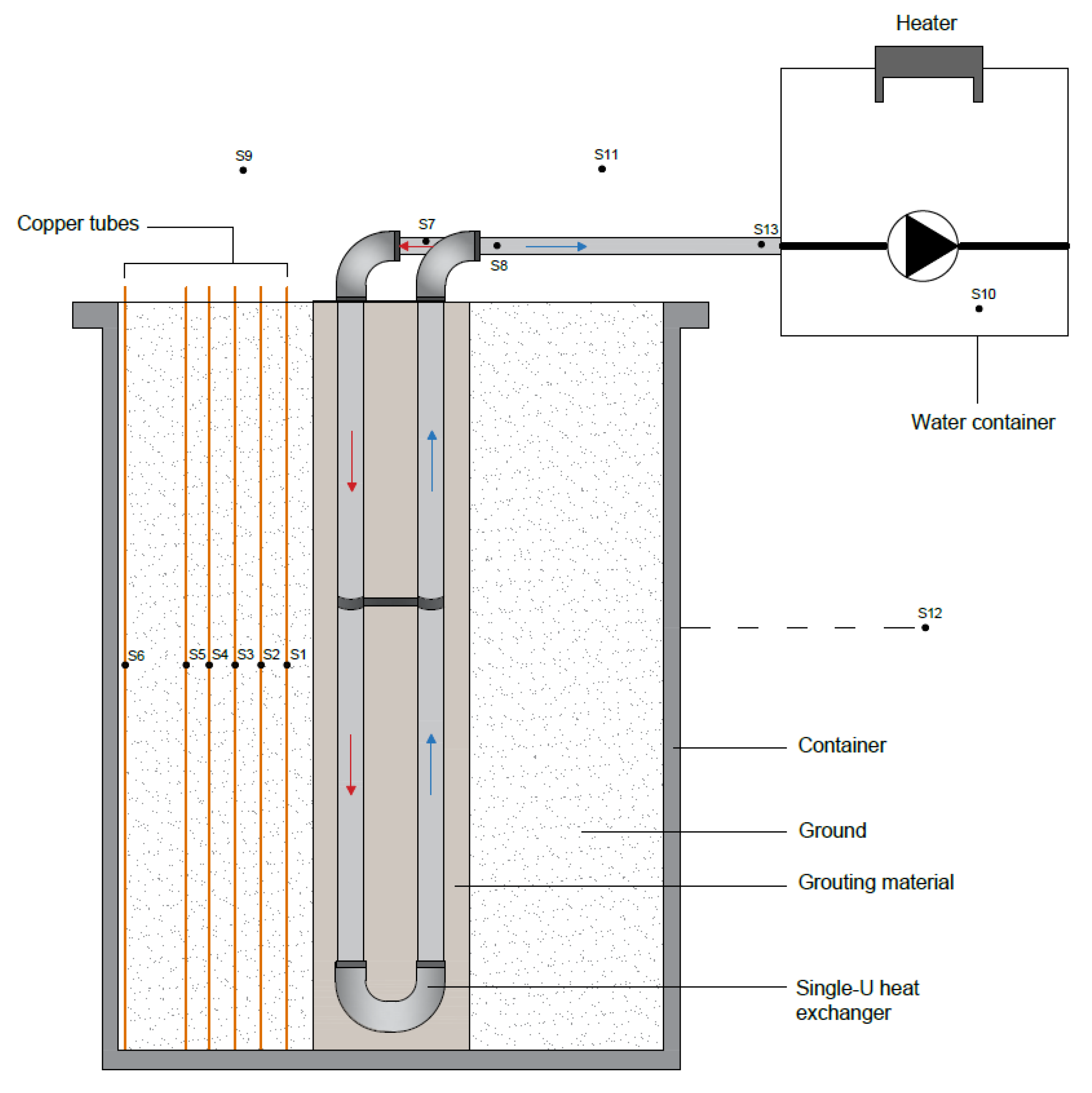
Six copper tubes of 10 mm diameter placed inside the sandy material and used to keep the temperature sensors to monitor this parameter along the study time at different distances from the vertical heat exchanger. One of the tubes was placed right next to the external container, while the other 5 were equally separated 41 mm thanks to the development of a fixed structure in a 3D printer.
Thirteen sensors set in several components of the experimental setup to monitor and control significant parameters for its proper performance: (i) 6 temperature sensors placed inside the copper tubes in the sandy material (S1 to S6), (ii) 2 temperature sensors to control this thermal parameter when the working fluid was driven in and outside the vertical single-U heat exchanger from the glass container (S7 and S8), (iii) 2 sensors to control the room temperature conditions during the study time (S9 and S11), (iv) 1 temperature sensor inside the glass container of the working fluid (S10), (v) 1 laser sensor to measure the external temperature of the main cylindrical container of the setup (S12), and (v) a flowmeter sensor to measure the flow rate of the system, placed right after an external valve that let control this parameter in the inlet heat-exchanger tube (S13).
Insulating polyurethane base with a thermal conductivity of 0.08 W/m·K placed on the bottom of the main container to avoid additional heating losses during the experiment. The top has been left without insulation to replicate the real conditions of the well field in typical geothermal installations.
Figure 1 presents a basic schema of the experimental setup described above with the aim of easily recognizing all the mentioned components. Additionally, Figure 2 shows the setup assembly process and the final appearance of the system.
It must be noted that the material filling was made following a specific procedure to ensure the homogeneity of the horizontal layers. As the previous Figure 1 shows, the temperature registers were made in a radial way (keeping the z coordinate constant) with the aim of avoiding different material density states probably derived from the gravity effect.

2.1.1. Temperature Control

As briefly mentioned above, the temperature was measured along several points of the analyzed geothermal setup every 5 s. For this purpose, DS18B20 temperature sensors with ±0.5 °C of accuracy were used. This set of sensors was connected to a unique device that recorded all the measured data in a removable memory card. Additionally, all measured parameters could be accurately controlled in the laboratory in real-time using a Wi-Fi connection in an external handheld machine from any standard mobile phone.
Specifically, the external temperature of the main polyethylene container that capsuled the entire structure was measured using an infrared sensor. This device measured both the external temperature of the container from a fixed distance and the room temperature of the working environment. Besides all the temperature sensors, a flowmeter sensor was also used to measure the flow rate in the circuit. Figure 1 showed the sensors’ location along the geothermal setup while Table 1 presents the measures taken by each sensor and the corrections applied.
Before starting the geothermal heat exchanging performance in the laboratory and hence measuring temperatures, sensors were calibrated so the corresponding correction factors were applied to each of them before carrying any other calculation. The flowmeter sensor was also tested in a smaller deposit in such a way that the flow rate measures were adjusted depending on the obtained results.
The ground temperature sensors (S1–S6) were set in the copper tubes of 10 mm diameter carefully placed in the ground of the main container.
Before using, all the temperature sensors were calibrated and the corresponding correction factors were applied to each of them. The flowmeter sensor was equally tested and adjusted in function of the results obtained during its calibration. Figure 3 shows the schema of the data acquisition system implemented in the experimental device.

2.1.2. Experimental Procedure

The experimental setup presented in this research was assembled with the aim of reproducing the same thermal phenomena that takes place in a real geothermal installation but on a laboratory scale. Given the limitations, the reproduced process was actually opposite to the one experienced in real installations. While the working fluid is normally ground-heated and flows through the heat exchanger, the developed system used a resistance placed in the glass tank that contained the water. Thus, the working fluid got heated inside the tank and cooled down while flowing through the heat exchanger in a close system.
Once the geothermal process started, the thermal response of the sandy filling material placed between the vertical borehole and the external container was evaluated using the temperature sensors previously described. The geothermal system worked for 6 entire days, being both the water pump and the heat resistance stopped in the middle of the study period. In this way, the thermal response of the sand both when the working fluid was exchanging heat and cooling down could be studied. Moreover, this approach eased determination of the stationary period.
Finally, the thermal conductivity of the sandy material was calculated following the existing theoretical basis, as being one of the most significant parameters that define the efficiency of the geothermal systems. Moreover, results were compared with those obtained using a commercial measuring device.

2.2. Theoretical Basis

The basis of the experiment consisted of providing a certain amount of heat through the heat-exchanger system to increase the temperature of the sand that filled the surroundings. Thus, the sand temperature was warmer when measured closer to the borehole and cooler down radially depending on the thermal conductivity of the material.
This thermal parameter was measured at certain distances to the geothermal borehole using the sensors placed inside the cupper tubes (S1 to S6). Given the system geometry, the heat transmission took place in a radial way so the proper mathematical model to analyze the system was based on cylindrical coordinates. Figure 4 shows the heat transmission and the location of the temperature sensors in the sand, with r1 to r5 as the distances from each sensor (S1 to S5) to the center of the vertical borehole.
The sandy material (ground) behaves as an insulating layer, so the heat transmitted through the first radial cylinder must be necessarily transferred through the second and so on. This behavior defined the developed experimental system as a series-resistive model. The general equation that defines the heat transmission is presented in cylindrical coordinates as Equation (1) and is further described in Figure 5.
1 r r ( k r   T r ) + 1 r 2 ( k T ) + z ( k T z ) + e ˙ g = ρ c T t
where
  • k = material thermal conductivity
  • r = radio
  • r = radio differential
  • = angle
  • = angle differential
  • z = height differential
  • p = material density
  • c = material specific heat
  • e ˙ g = energy generated
  • T = temperature differential
  • t = time differential
Once the boundary restrictions are considered, integrating and applying the Dirichlet border condition in the two lateral areas of the cylinder, the following Equation (2) is obtained.
T ( r ) =   ( l n ( r / r 1 ) l n ( r 2 / r 1 ) ) ( T 2 T 1 ) + T 1
In this way, the heat rate through a cylinder can be defined as follows:
Q ˙ =   k A d T d r     Q ˙ = 2 π k L T 1 T 2 l n ( r 2 / r 1 )
As the usual practice uses the concepts of thermal resistance and thermal circuit in analogy to electric circuits, Equation (4) is deduced.
Q ˙ = Δ T R T
where
  • Q ˙ = Heat rate equivalent to the electrical power
  • Δ T = Temperature difference (T1 − T2) comparable to the potential difference in an electric circuit
  • RT = Thermal resistance
    L = Borehole length
All the above allows writing the previous Equation (4) as follows:
Q ˙ =   T 1 T 2 ( l n ( r 2 / r 1 ) 2 π k L )
Thus, the thermal resistance could be obtained as shown in Equation (6).
R T = l n ( r 2 / r 1 ) 2 π k L

2.2.1. Model Validation

The validation of the theoretical model applied on the developed geothermal setup was based on the measurements made with the temperature sensors S1–S5. As previously stated, the thermal resistances were based on a series resistive cylindrical system so the following expression (Equation (7)) had to be verified.
Q ˙ =   T 1 T 2 ( l n ( r 2 / r 1 ) 2 π k L ) = T 2 T 3 ( l n ( r 3 / r 2 ) 2 π k L )
In this way, if the model is correct, when the permanent regime is reached, the equalities presented in Equations (8)–(10) must be also satisfied.
T 3 T 2 T 2 T 1 = l n ( r 3 / r 2 ) l n ( r 2 / r 1 )                 T 3 T 2 T 2 T 1 l n ( r 3 / r 2 ) l n ( r 2 / r 1 ) = 0
T 4 T 3 T 3 T 2 = l n ( r 4 / r 3 ) l n ( r 3 / r 2 )                 T 4 T 3 T 3 T 2 l n ( r 4 / r 3 ) l n ( r 3 / r 2 ) = 0
T 5 T 4 T 4 T 3 = l n ( r 5 / r 4 ) l n ( r 4 / r 3 )                 T 5 T 4 T 4 T 3 l n ( r 5 / r 4 ) l n ( r 4 / r 3 ) = 0

2.2.2. Temperature Sensors Calibration

The temperature sensors used in the several tests performed for this experiment were thoroughly calibrated beforehand (Section 2.1.1). With that aim, all these sensors were actively measuring the same room and location during a certain period of time. Despite the fact that sensors do not need calibration, temperature tests were made to determine the possible measurement deviation among sensors. These measurements are graphically represented in Figure 6.
The calibration of the sensors considering the measurements previously presented was performed as follows:
Calculation of the average value read by each sensor.
Determination of the difference between the mean value and the sensor measurement for each reading.
For each sensor, calculation of the mean value of the difference estimated in the previous step. This average value represented the correction factor to be applied to the measurement of each sensor. These factors can be observed in Table 2.
Additionally, the standard deviation of each sensor measurement regarding the mean temperature value was calculated using the expression of Equation (11).
σ = σ 2 = ( x μ ) 2 N
where
  • σ = deviation
  • x = Temperature sensor measurement
  • μ = Mean value from the set of measurements of each sensor
As a result of the individual calculation of the deviation of each sensor in each reading, the total deviation associated to the measurement of each temperature sensor is shown in Table 3. These deviations are only an indication of the relative quality of the measurements acquired. It is a way of controlling the possible deviation respect to the real value depending on which sensor the measurement comes from.

2.3. Experimental Phase

Once the setup was installed and after making all the corresponding verifications and calibrations, the experimental workflow was carried out following the sequence described in Figure 7.

Thermal Conductivity Characterization

The thermal conductivity of a certain material is a constant parameter supposing a homogeneous and isotropic medium. Effective thermal conductivity of the surrounding ground is the foremost parameter for geothermal applications [31]. Thus, experimental models and measurements are required to both understand and verify the results obtained following the theoretical basis, comparing it to commercial measurement instruments. All measurements were taken in a model that, even on a laboratory scale, reproduced the working flow of a real geothermal installation. Moreover, this experiment was a great alternative to measure and analyse the thermal properties of the soil in an inexpensive and more effective way than using thermal response tests (TRTs) on a real installation [32].
The estimation of this property in the ground that constitutes the experimental setup derives from the determination of the thermal resistance between two points. To obtain these thermal resistances, the heat transfer that goes through the model must be defined. With that aim, the following Equation (12) was implemented.
Q ˙ = m ˙ c p ( T i T o )
where
  • Q ˙ = Heat rate
  • m ˙ = mass flow rate (kg/s)
  • cp = working fluid specific heat
  • Ti = inlet temperature
  • To = outlet temperature
From the flow rate (m3/h) established in the pump, the mass flow rate can be directly obtained using the following Equation (13).
m ˙ [ k g s ] = F   [ m 3 h ] · p [ k g m 3 ] · [ 1   h 3600   s ]
Finally, calculating the thermal resistance applying Equation (6), the thermal conductivity is deduced by the expression of Equation (14):
k = l n ( R 2 R 1 ) 2 π R T L

3. Results

3.1. Preliminary Test

After several experimental tests trying to define the correct operation of the geothermal device, in the final test, the setup was working for a period of time of approximately six days. In the third day of the experiment, the water pump and the heating device were disconnected but the sensors continued measuring. In this way, the response of the ground was evaluated during the fluid circulation and heating and during the cooling down with no fluid flowing. As already described in the workflow (Figure 7), the water tank was heated by the thermal resistance before connecting the set of sensors.
Results of the complete tests are represented in Figure 8, where all the measurements of the temperature sensors are shown. Additionally, Figure 9 shows the flow rate during the same test period. The water pump was paused working around the mid-term of the total experimental test, and hence, the flow rate was radically reduced to zero (Figure 9). Water flow rate was established from different preliminary tests that allowed the establishment of the most appropriate system performance and conditions.
As can be observed in Figure 9, the water pump was paused around mid-term of the total experimental test, the moment in which the flow rate is reduced to zero.
The following step consisted of determining when the permanent regime was achieved. This regime is settled when all the temperatures values remain quite constant, without remarkable variations in time (below 10%). Finally, applying the correction factors presented in Table 2 for temperature sensors S1–S10, the corrected temperature measurements can be graphically observed in Figure 10.

3.2. Validation

As explained in Section 2.2.1, the developed geothermal model must satisfy Equations (8)–(10). Thus, these calculations were determined once detected and corrected the permanent regime (Figure 10).
In the setup built to perform the present research, distances (r1–r5) mentioned in Equations (8)–(10) and graphically represented in Figure 4 have the values contemplated in Table 4.
Considering that the temperatures measured by the temperature sensors should remain timely constant in the permanent regime according to its definition, already corrected data from a certain instant of this period were used for the model validation. The fixed temperature values used are collected in Table 5.
Based on the data of the previous Table 4 and Table 5, the results of each of the terms of Equations (8)–(10) are presented in Table 6.
The difference between the first and second terms of each equation (Equations (8)–(10)) should be zero. As observed in Table 6, these differences are quite low, representing errors of less than the decimal point (10%), meaning that it is correct to assume that the system reached the steady state (also verified by Figure 10). In this way, the developed model was considered valid for performing the corresponding analysis of the geothermal exchange in a borehole. From the validation of this model, numerous studies could be carried out. This research considered the estimation of the thermal conductivity of the material used as a surrounding ground as it is a crucial parameter that determines the heat transmission and hence the installation efficiency [31].

3.3. Estimation of the Ground Thermal Conductivity

As already mentioned, the final aim of this work is calculating the thermal conductivity of the surrounding material that represents the ground on a real geothermal installation. In this way, this was the approach selected among the multiple applications of the experiment. Temperatures measured by sensors S1–S5 were the basis for this estimation. Figure 11 shows the evolution of the heat transfer process between the working fluid and the surrounding material based on the data recorded by sensors S1–S5.
Heat transmission variations were really notable during the first stages of the experiment (stages 1 to 6 in Figure 11) and were almost imperceptible afterwards (stages 6 to 12) (Figure 11). This fact was due to the gradual appearance of the permanent regime in the second half of the study.
Based on the corrected temperature values recorded by sensors S1–S5 during the permanent regime (Figure 10) and the theoretical basis (Section 2.2), the thermal conductivity of the surrounding material was estimated following the next steps:
Determination of the mass flow rate and heat rate using Equations (12) and (13). Data of a certain instant from the set of corrected temperature results in the permanent regime (inlet and outlet fluid temperatures) were used to calculate the mentioned parameters. Table 7 presents all the required parameters and the results of the mass flow rate and heat rate. As this Table shows, the difference between the temperature of the inlet and outlet fluid is 0.18 °C. Since the BHE constituting the proposed apparatus is just one meter long, higher differences are not possible because of scale limitations. It should be also noted that previous tests allowed verifying that lower flow rates did not contribute to increasing the mentioned temperature difference. With reduced flow rates, the fluid behaved in laminar regime, reducing the thermal exchange among pipes, grouting material, and ground, making the temperature between inlet and outlet fluids even lower.
Calculation of the thermal resistances of the material found between sensors S1–S2, S2–S3, S3–S4, and S4–S5. The expression presented in Equation (4) was used with that aim. Results are shown in Table 8.
Determination of the ground thermal conductivity applying Equation (14). This calculation, also made for the material contained between the couple of sensors S1–S2, S2–S3, S3–S4, and S4–S5, is based on the thermal resistances presented in Table 8. The results of the thermal conductivity parameter can be found in Table 9.

4. Discussion

This paper presents an experimental setup that is capable of determining the thermal conductivity of the surrounding material of the borehole heat exchanger. After validating the developed model, the temperature values recorded by a set of sensors placed at several distances from the main geothermal heat exchanger were used to calculate the ground thermal conductivity. This parameter was estimated for several sections of the material applying the same mathematical procedure. The average value obtained was 0.543 W/m·K (Table 9), with a standard deviation of 0.001 W/m·K.

KD2 Pro Measurement

Even obtaining a clearly low value for the standard deviation and hence quite a proper result for the thermal conductivity, which demonstrated the validity of the developed system, a supplementary method was also applied and compared. Thus, KD2 Pro device was used on the same sandy material and under the same conditions. It is a thermal properties analyzer developed by Decagon Devices [28] that allows the measurement of the thermal resistivity or the thermal conductivity of a certain rocky material. In this case, the portable controller was connected to the sensor RK-1, usually named as “needle probe”. Based on the infinite line heat source theory, heat is applied to the needle for a set heating time and the temperature is measured in the monitoring needle during heating and for an additional time after the heating period. Expressions applied for the computation during heating and cooling are shown in Equations (15) and (16). Additionally, Equation (17) presents the way of computing the thermal conductivity [33,34,35].
T =   m 0 + m 2 t +   m 3 l n t
T =   m 1 + m 2 t + m 3 l n t t t h
k = q 4 m 3
where
  • m0 is the ambient temperature during heating
  • m2 is the rate of background temperature drift
  • m3 is the slope of a line relating temperature rise to logarithm of temperature
  • q is the heat flux applied to the needle probe for a certain set of time
RK-1 sensor (3.9 mm in diameter, 6 cm in length, and ±10% of accuracy) was used in this work to measure the thermal conductivity of the material placed in the experimental device holding the same role as the ground in a real geothermal installation. Since this thermal parameter is affected by the state of compaction, the measurement was carried out in several levels to finally obtain a representative value of the whole volume contained in the experimental setup. This is the only way the level of compaction could be equaled in both methods towards a valid comparison. Thus, KD2 Pro was used in different locations: at the surface and at the depths of 25 cm, 50 cm, and 75 cm. The bottom of the experiment could not be reached due to the limited length of the sensor cable. Figure 12 shows one of the measuring processes taken with KD2 Pro.
The results obtained are shown in Table 10. It is worth noting that each measurement was made three times, calculating the mean value for each location.
In order to estimate the measurement that this device would determine in the deepest level of the container, the relation between the thermal conductivity and depth (directly related with the level of compaction of the material due to the weight of material supported) was graphically obtained (Figure 13). Thus, applying the equation that relates both variables, a thermal conductivity value of 0.676 W/m·K was obtained for the depth of 100 cm (bottom of the container).
Finally, the mean value for all the values of Table 10 and the one deduced from them was calculated. In this way, the thermal conductivity of the material used as ground in the suggested experiment takes the value of 0.522 W/m·K ± 0.01 W/m·K by applying KD2 Pro procedure.
As way of comparison, Figure 14 represents the thermal conductivity value obtained from three procedures: the suggested experimental setup (0.543 W/m·K), the KD2 Pro device (0.522 W/m·K), and a standard tabulated value for a dry sandy material (0.582 W/m·K) [36].
Observing Figure 14, the thermal conductivity result obtained from the implementation of the experimental setup is similar to the one coming from the use of KD2 Pro equipment (0.543 W/m·K and 0.522 W/m·K, respectively). Both solutions were obtained by measuring the thermal parameter of the material in the same conditions, and the low difference of values (0.021 W/m·K) could be attributed to the limitation of the KD2 Pro to measure at all levels of the medium. Low deviations are also indicative of proper system operation beyond the scale and geometric limits derived from its design.
Regarding the standard tabulated value, it is highly conditioned by the measuring conditions (ambient temperature, material humidity, compaction, etc.). Thus, obtaining the same value would not be realistic since the probabilities that the conditions of the material in the experimental test are equal to the conditions of the sandy material considered in the standard table are low.

5. Conclusions

It is important to accurately study the actual thermal exchange between the ground and the geothermal components in order to design Ground Source Heat Pumps (GSHPs). The development of this experimental device offers new approaches for analyzing the different thermal parameters that define the geothermal field. In this first research, the design of the system was both tested and validated from the physical model and applied in the calculation of the thermal conductivity parameter. Thus, as an example of the several applications this device could have, the thermal conductivity of the surrounding sandy material (ground-role) was estimated from the temperature sensors measurements. The agreement found among the thermal conductivity results obtained from the different sections defined by the set of sensors initially confirmed the system validity. For a more consistent corroboration, KD2 Pro equipment was also used on the same material and conditions. The final thermal conductivity value obtained using this instrument highly corresponded to the experimental setup results.
In addition to this application that allows both calculating and monitoring of the thermal conductivity of the ground, future researches will analyze other essential factors that thoroughly affect the geothermal behavior and hence the system efficiency. In the short term, the following studies are expected:
Modification of the original state of the sandy material used as geothermal ground. Different humidity states will be applied, and the evolution of the thermal conductivity parameter will be analyzed.
Application of different flow rates (controlling them using the valve installed in the system) and study of the thermal exchange and fluid circulation regime.
Use of new working fluids, varying the content of glycol and analysis of the influence of each fluid in the thermal behavior.
Study of the minimum distances among the boreholes of a certain geothermal system. Results from the laboratory device could be a valuable reference in real GSHP installations and heat-exchange affection between neighbor boreholes.
Finally, it must be clarified that, despite the fact that the proposed experimental device constitutes a useful tool to understand the phenomena taking part in the geothermal exchange, it cannot be considered as a substitute of the TRT. Nevertheless, it constitutes a preliminary step in the estimation of the ground thermal conductivity, resulting from special interest when in situ tests (as the TRT) are not viable. Beyond this application, the apparatus is also valuable to perform different analyses on the ground as an approach to understand the thermal phenomena that take place in low enthalpy geothermal systems (as the ones detailed before).

Author Contributions

All authors performed the experimental and theoretical basis of the research. C.S.B., L.P.M, I.M.N., and J.F.-H. implemented the methodology and calculations and analyzed the results. A.F.M., S.L., and D.G.-A. provided technical and theoretical support. C.S.B. wrote the manuscript and all authors read and approved the final version. All authors have read and agreed to the published version of the manuscript.

Funding

This research received no external funding.

Acknowledgments

Authors would like to thank the Department of Cartographic and Land Engineering of the Higher Polytechnic School of Avila, University of Salamanca, for allowing us to use their facilities and for their collaboration during the experimental phase of this research. In addition, authors would like to thank Iberdrola S.L. and the University of Salamanca for the support given through Cátedra Iberdrola VIII Centenario. The authors would also like to thank the Ministry of Education, Culture, and Sport, the University of Salamanca and the Santander Bank for providing an FPU Grant and a predoctoral grant to some of the authors of this paper.

Conflicts of Interest

The authors declare no conflict of interest.

Nomenclature

Symbols
kMaterial thermal conductivity [W/m·K]
rRadio [m]
rRadio differential [m]
Angle [°]
Angle differential [°]
zHeight differential [m]
t Time differential [s]
pMaterial density [kg/m3]
cMaterial specific heat [J/kg°C]
e ˙ g Energy generated [J]
TTemperature differential [°C]
LBorehole length [m]
Q ˙ Heat rate [W]
FFlow rate [m3/h]
Δ T Temperature difference [°C]
RTThermal resistance [m·K/W]
σ Deviation
xTemperature sensor measurement [°C]
μ Mean value from the set of measurements of each sensor [°C]
m ˙ Mass flow rate [kg/s]
cpWorking fluid specific heat [J/kg°C]
TiInlet temperature [°C]
ToOutlet temperature [°C]
m0Ambient temperature during heating [K]
m2Rate of background temperature drift [K]
m3Slope of a line relating temperature rise to logarithm of temperature [K]
q ˙ Heat flux applied to the needle probe for a certain set of time [W/m]
Acronyms
GSHPGround Source Heat Pump
HPHeat Pump
BHEBorehole Heat Exchanger

References

  1. Self, S.J.; Reddy, B.V.; Rosen, M.A. Geothermal heat pump systems: Status review and comparison with other heating options. Appl. Energy 2013, 101, 341–348. [Google Scholar] [CrossRef]
  2. Esen, H.; Inalli, M.; Esen, M. A techno-economic comparison of ground-coupled and air-coupled heat pump system for space cooling. Build. Environ. 2007, 42, 1955–1965. [Google Scholar] [CrossRef]
  3. Blázquez, C.S.; Nieto, I.M.; Martín, A.F.; González-Aguilera, D. Optimization of the Dimensioning Process of a Very Low Enthalpy Geothermal Installation. In Smart Cities, Proceedings of the ICSC-CITIES 2018, Soria, Spain, 26–27 September 2018; Nesmachnow, S., Hernández Callejo, L., Eds.; Communications in Computer and Information Science; Springer: Cham, Switzerland, 2019; Volume 978, pp. 179–191. [Google Scholar]
  4. Bauer, D.; Heidemann, W.; Diersch, H.J. Transient 3D analysis of borehole heat exchanger modeling. Geothermics 2011, 40, 250–260. [Google Scholar] [CrossRef]
  5. Blázquez, C.S.; Martín, A.F.; García, P.C.; Pérez, L.S.S.; Caso, S.J.d. Analysis of the process of design of a geothermal installation. Renew. Energy 2016, 89, 1–12. [Google Scholar] [CrossRef]
  6. Sáez Blázquez, C.; Farfán Martín, A.; Martín Nieto, I.; Carrasco García, P.; Sánchez Pérez, L.S.; González-Aguilera, D. Efficiency Analysis of the Main Components of a Vertical Closed-Loop System in a Borehole Heat Exchanger. Energies 2017, 10, 201. [Google Scholar] [CrossRef] [Green Version]
  7. Al-Khoury, R.; Bonnier, P.G.; Brinkgreve, R.B. Efficient finite element formulation for geothermal heating system. Part I: Steady state. Int. J. Numer. Methods Eng. 2005, 63, 988–1013. [Google Scholar] [CrossRef]
  8. Al-Khoury, R.; Bonnier, P.G. Efficient finite element formulation for geothermal heating system. Part II: Transient. Int. J. Numer. Methods Eng. 2005, 67, 725–745. [Google Scholar] [CrossRef]
  9. Carlini, M.; Castellucci, S.; Allegrini, E.; Tucci, A. Down-Hole Heat Exchangers: Modelling of a Low-Enthalpy Geothermal System for District Heating. Math. Probl. Eng. 2012, 2012, 1–11. [Google Scholar] [CrossRef]
  10. Green, D.L. Modelling Geomorphic Systems: Scaled Physical Models. Section 5.3; In Geomorphological Techniques; Cook, S.J., Clarke, L.E., Nield, J.M., Eds.; British Society for Geomorphology: London, UK, 2014. [Google Scholar]
  11. Volkov, A.V.; Ryzhenkov, A.V.; Kurshakov, A.V.; Grigoriev, S.V.; Bekker, V.V. Physical Modelling of Temperature’s Potential Decrease for Near-Wellbore Rocks during Extraction of Thermal Energy. Int. J. Appl. Eng. Res. 2017, 12, 6570–6575. [Google Scholar]
  12. Scotton, P.; Teza, G.; Santa, G.D.; Galgaro, A.; Rossi, D. An experimental setup to measure the heat-exchange processes by controlling thermal and hydraulic conditions. Igshpa Res. Track Stockh. 2018, 18–20. [Google Scholar] [CrossRef]
  13. Ebeling, J.C.; Kabelac, S.; Luckmann, S.; Kruse, H. Simulation and experimental validation of a 400 m vertical CO2 heat pipe for geothermal application. Heat Mass Transf. 2017, 53, 3257–3265. [Google Scholar] [CrossRef]
  14. Sivasakthivel, T.; Murugesan, K.; Kumar, S.; Hu, P.; Kobiga, P. Experimental study of thermal performance of a ground source heatpump system installed in a Himalayan city of India for compositeclimatic conditions. Energy Build. 2016, 131, 193–206. [Google Scholar] [CrossRef]
  15. Postrioti, L.; Baldinelli, G.; Bianchi, F.; Buitoni, G.; Maria, F.D.; Asdrubali, F. An experimental setup for the analysis of an energy recovery system from wastewater for heat pumps in civil buildings. Appl. Therm. Eng. 2016, 102, 961–971. [Google Scholar] [CrossRef]
  16. Golasi, I.; Salata, F.; Coppi, M.; Vollaro, E.d.L.; Vollaro, A.d.L. Experimental Analysis of Thermal Fields Surrounding Horizontal Cylindrical Geothermal Exchangers. Energy Procedia 2015, 82, 294–300. [Google Scholar] [CrossRef] [Green Version]
  17. Remund, C.P. Borehole thermal resistance: laboratory and field studies. Ashrae Trans. 1999, 105, 439. [Google Scholar]
  18. Kramer, C.A.; Ghasemi-Fare, O.; Basu, P. Laboratory thermal performance tests on a model heat exchanger pile in sand. Geotech. Geol. Eng. 2015, 33, 253–271. [Google Scholar] [CrossRef]
  19. Salim Shirazi, A.; Bernier, M. A small-scale experimental apparatus to study heat transfer in the vicinity of geothermal boreholes. HvacR Res. 2014, 20, 819–827. [Google Scholar] [CrossRef]
  20. Luo, J.; Rohn, J.; Xiang, W.; Bayer, M.; Priess, A.; Wilkmann, L.; Zorn, R. Experimental investigation of a borehole field by enhanced geothermal response test and numerical analysis of performance of the borehole heat exchangers. Energy 2015, 84, 473–484. [Google Scholar] [CrossRef]
  21. Harlé, P.; Kushnir, A.R.; Aichholzer, C.; Heap, M.J.; Hehn, R.; Maurer, V.; Duringer, P. Heat flow density estimates in the Upper Rhine Graben using laboratory measurements of thermal conductivity on sedimentary rocks. Geotherm. Energy 2019, 7, 1–36. [Google Scholar] [CrossRef]
  22. Lyne, Y.; Paksoy, H.; Farid, M. Laboratory investigation on the use of thermally enhanced phase change material to improve the performance of borehole heat exchangers for ground source heat pumps. Int. J. Energy Res. 2019, 43, 4148–4156. [Google Scholar] [CrossRef]
  23. Nieto, I.M.; Martín, A.F.; Blázquez, C.S.; Aguilera, D.G.; García, P.C.; Vasco, E.F.; García, J.C. Use of 3D electrical resistivity tomography to improve the design of low enthalpy geothermal systems. Geothermics 2019, 79, 1–13. [Google Scholar] [CrossRef]
  24. Blázquez, C.S.; Martín, A.F.; Nieto, I.M.; García, P.C.; Pérez, L.S.S.; Aguilera, D.G. Thermal conductivity map of the Avila region (Spain) based on thermal conductivity measurements of different rock and soil samples. Geothermics 2017, 65, 60–71. [Google Scholar] [CrossRef]
  25. Blázquez, C.S.; Martín, A.F.; Nieto, I.M.; González-Aguilera, D. Measuring of Thermal Conductivities of Soils and Rocks to Be Used in the Calculation of a Geothermal Installation. Energies 2017, 10, 795. [Google Scholar] [CrossRef]
  26. Blázquez, C.S.; Martín, A.F.; García, P.C.; González-Aguilera, D. Thermal conductivity characterization of three geological formations by the implementation of geophysical methods. Geothermics 2018, 72, 101–111. [Google Scholar] [CrossRef]
  27. Zeng, H.Y.; Diao, N.R.; Fang, Z.H. A finite line source model for boreholes in geothermal heat exchangers. Heat Transf.—Asian Res. Cosponsored Soc. Chem. Eng. Jpn. Heat Transf. Div. Asme 2002, 31, 558–567. [Google Scholar] [CrossRef]
  28. Devices, D. KD2 Pro Thermal Properties Analyser Operator’s Manual; Decagon Devices, Inc.: Pullman, WA, USA, 2016. [Google Scholar]
  29. Blázquez, C.S.; Martín, A.F.; Nieto, I.M.; García, P.C.; Pérez, L.S.S.; González-Aguilera, D. Analysis and study of different grouting materials in vertical geothermal closed-loop systems. Renew. Energy 2017, 114, 1189–1200. [Google Scholar] [CrossRef]
  30. ÇENGEL, Y. Transferencia de Calor y de Masa, un Enfoque Práctico, 3rd ed.; Editorial McGraw-Hill: Mexico City, México, 2007. [Google Scholar]
  31. Jia, G.S.; Tao, Z.Y.; Meng, X.Z.; Ma, C.F.; Chai, J.C.; Jin, L.W. Review of effective thermal conductivity models of rock-soil for geothermal energy applications. Geothermics 2019, 77, 1–11. [Google Scholar] [CrossRef]
  32. Li, M.; Zhang, L.; Liu, G. Estimation of thermal properties of soil and backfilling material from thermal response tests (TRTs) for exploiting shallow geothermal energy: Sensitivity, identifiability, and uncertainty. Renew. Energy 2019, 132, 1263–1270. [Google Scholar] [CrossRef]
  33. Carslaw, H.S.; Jaeger, J.C. Conduction of Heat in Solid, 2nd ed.; Oxford University Press: Oxford, UK, 1959. [Google Scholar]
  34. Kluitenberg, G.J.; Ham, J.M.; Bristow, K.L. Error analysis of the heat pulse method for measuring soil volumetric heat capacity. Soil Sci. Soc. Am. J. 1993, 57, 1444–1451. [Google Scholar] [CrossRef]
  35. Shiozawa, S.; Campbell, G.S. Soil thermal conductivity. Remote Sens. Rev. 1990, 5, 301–310. [Google Scholar] [CrossRef]
  36. Propiedades Termicas de Algunos Materiales de Construccion y Aislantes. Informes de la Construcción, Universidad de Buenos Aires, Facultad de Ingeniería. Available online: http://materias.fi.uba.ar/6731/Tablas/Tabla6.pdf (accessed on 16 January 2020).
Figure 1. Schema of the geothermal setup reproduced in the laboratory.
Energies 13 01270 g001
Figure 2. Installation of the experimental setup: (A) Thermal insulation of the main container, (B) main container and first cupper tube, (C) geothermal borehole placement, (D) Set of cupper tubes set to equal distances, and (E) overview of the setup with all the sensors and accessories.
Energies 13 01270 g002
Figure 3. Schema of the data acquisition system.
Energies 13 01270 g003
Figure 4. Heat transmission through the ground system and temperature sensors location.
Energies 13 01270 g004
Figure 5. A differential volume element in cylindrical coordinates [30].
Energies 13 01270 g005
Figure 6. Temperature sensors measuring in a common ambient for the corresponding calibration.
Energies 13 01270 g006
Figure 7. Description of the experimental methodology followed on the geothermal device.
Energies 13 01270 g007
Figure 8. Measurements of the set of temperature sensors used in the experimental setup.
Energies 13 01270 g008
Figure 9. Flow rate during the test carried out on the experimental setup.
Energies 13 01270 g009
Figure 10. Corrected temperature measurements in the permanent regime by applying the correction factors on sensors S1–S10. (Note that S7 measurements are hidden due to their coincidence with the measurements from S8).
Energies 13 01270 g010
Figure 11. Heat transfer between the working fluid (water) and the surrounding material (silica sand with 15% humidity) according to the temperature values recorded by sensors S1–S5: Step 1 = 21,600 s, step 2 = 43,200 s, step 3 = 64,800 s, step 4 = 86,400 s, step 5 = 108,000 s, step 6 = 129,600 s, step 7 = 151,200 s, step 8 = 172,800 s, step 9 = 194,400 s, step 10 = 216,000 s, step 11 = 237,600, and step 12 = 259,200.
Energies 13 01270 g011
Figure 12. Measuring the ground thermal conductivity using KD2 Pro equipment and RK-1 sensor.
Energies 13 01270 g012
Figure 13. Relation between the thermal conductivity of the material and the depth where the parameter was measured.
Energies 13 01270 g013
Figure 14. Thermal conductivity of the sandy material obtained from the experimental setup, the KD2 Pro device, and the standard tabulated value.
Energies 13 01270 g014
Table 1. Description of the temperature sensors used in the experimental device.
Sensor IdentificationSensor ModelMeasurementUnit of Measure
S1DS18B20Ground temperature°C
S2DS18B20Ground temperature°C
S3DS18B20Ground temperature°C
S4DS18B20Ground temperature°C
S5DS18B20Ground temperature°C
S6DS18B20Ground temperature°C
S7DS18B20Inlet fluid temperature°C
S8DS18B20Outlet fluid temperature°C
S9DS18B20Ambient temperature°C
S10DS18B20Fluid temperature in the heater container°C
S11MLX90614Ambient temperature°C
S12MLX90614External container temperature°C
S13YF-S201Flow rateL/h
Table 2. Correction factors to be implemented in the temperature measurement of each sensor.
SensorS1S2S3S4S5S6S7S8S9S10
Correction Factor (°C)−0.040.180.28−0.31−0.030.010.09−0.090.03−0.12
Table 3. Deviations of each sensor measurement in relation to the mean value.
SensorS1S2S3S4S5S6S7S8S9S10
Deviation0.040.180.280.310.040.020.090.100.040.12
Table 4. Distances of sensors S1–S5 to the center of the cylinder tank used to hold the geothermal experimental device.
Distancesr1r2r3r4r5
(mm)126.8167.8208.8249.8290.8
Table 5. Temperature values of sensors S1–S5 for a certain moment of the permanent regime.
TemperaturesT1T2T3T4T5
(°C)37.734.231.429.327.4
Table 6. Results of each term of Equations (8)–(10), differences, and errors.
EquationsFirst Term (°C)Second Term (mm)DifferenceError * (%)
Equation (8) T 3 T 2 / T 2 T 1 ln ( r 3 / r 2 ) / ln ( r 2 / r 1 ) 0.022.50
0.8000.780
Equation (9) T 4 T 3 / T 3 T 2 ln ( r 4 / r 3 ) / ln ( r 3 / r 2 ) −0.079.33
0.7500.820
Equation (10) T 5 T 4 / T 4 T 3 ln ( r 5 / r 4 ) / ln ( r 4 / r 3 ) 0.066.63
0.9050.848
* Error is obtained from the expression: (Difference/First term) ∗ 100.
Table 7. Calculation of the mass flow rate and heat rate ( m ˙ ,   Q ˙ )
Q (m3/h) p (kg/m3) T i (°C) T o (°C) m ˙ (kg/s) Q ˙ (W)
0.182100047.3147.130.05142.325
Table 8. Thermal resistances for the material included between sensors S1–S2 (R1-2), S2–S3 (R2-3), S3–S4 (R3-4), and S4–S5 (R4-5).
R1-2 (m·K/W) R2-3 (m·K/W) R3-4 (m·K/W) R4-5 (m·K/W)
0.0830.0660.0490.045
Table 9. Thermal conductivities of the surrounding material obtained from the measurement of sensors S1–S5.
k1-2 (W/m·K) k2-3 (W/m·K) k3-4 (W/m·K) k4-5 (W/m·K)
0.5350.5270.5760.535
Table 10. Thermal conductivity results from the KD2 Pro measuring in each of the established depth positions.
Thermal
Conductivities
Position 1 (Surface)Position 2 (25 cm)Position 3 (50 cm)Position 4 (75 cm)
K1 (W/m·K)0.2820.3560.3980.462
K2 (W/m·K)0.2910.3520.4010.475
K3 (W/m·K)0.2860.3650.4100.466
Mean Value (W/m·K)0.2860.3580.4030.468

