In-Situ Stress Measurements at the Utah Frontier Observatory for Research in Geothermal Energy (FORGE) Site

Abstract

A scientific injection campaign was conducted at the Utah Frontier Observatory for Research in Geothermal Energy (FORGE) site in 2017 and 2019. The testing included pump-in/shut-in, pump-in/flowback, and step rate tests. Various methods have been employed to interpret the in-situ stress from the test dataset. This study focuses on methods to interpret the minimum in-situ stress from step rate, pump-in/extended shut-in tests data obtained during the stimulation of two zones in Well 58-32. This well was drilled in low-permeability granitoid. A temperature of 199 °C was recorded at the well’s total depth of 2297 m relative to the rotary Kelly bushing (RKB). The lower zone (Zone 1) consisted of 46 m of the openhole at the toe of the well. Fractures in the upper zone (Zone 2) were stimulated between 2123–2126 m measured depths (MD) behind the casing. The closure stress gradient variation depended on the depth and the injection chronology. The closure stress was found to increase with the pumping rate/volume. This stress variation could indicate that poroelastic effects (“back stress”) and the presence of adjacent natural fractures may play an important role in the interpretation of fracture closure stress. Further, progressively increasing local total stresses may, consequently, have practical applications when moderate volumes of fluid are injected in a naturally fractured or high-temperature reservoir. The alternative techniques that use pump-in/flowback tests and temperature signatures provide a valuable perspective view of the in-situ stress measurements.

1. Introduction

Enhanced geothermal systems (EGS) offer the potential to bring low-cost geothermal energy to locations that lack natural permeability. Permeability enhancement and the formation of EGS reservoirs can be accomplished through hydraulic or thermal stimulations. Although EGS development has been pursued throughout the world since the late 1970s, no commercial-scale EGS reservoirs have been developed. In 2018, the U.S. Department of Energy selected a location in south-central Utah near the rural community of Milford to develop and test the techniques required for creating, sustaining, and monitoring EGS reservoirs [1]. The centerpiece of the Frontier Observatory for Research in Geothermal Energy (FORGE) will consist of two deep, highly deviated wells drilled into low-permeability granite. Temperatures near 225 °C are anticipated at the total depth of the wells.

In-situ stresses, especially the minimum (often horizontal) total principal stress, are one of the key parameters required to optimize hydraulic fracturing design. In 2017 and 2019, a suite of injection activities was conducted in a pilot well, Well 58-32, at the FORGE site to assess the in-situ stress and other reservoir properties. These injection activities included pump-in/shut-in, pump-in/flowback, and step rate tests. For decades, various methods have been employed to infer in-situ stresses, mainly from pump-in/shut-in [2] and step rate tests. Various methods have been utilized to determine the fracture closure pressure, including G function analysis [3,4,5], plotting pressure vs. $\sqrt{t}$, and diagnostic log-log plots using pressure during extended shut-ins. It can also be inferred from ISIP (instantaneous shut-in pressure) [5,6] and reopening pressure. Fracture closure pressure is the in-fracture fluid pressure at closure, which is associated with the minimum total principal (often horizontal) in-situ stress.

At the FORGE site, the inferred in-situ stresses vary with different injection cycles (in two separate stress measurement campaigns where multiple injection-shut-in or injection-flowback cycles were performed) in different zones along the length of a vertical well drilled in a relatively uniform granitoid. The variations of inferred in-situ stresses were investigated, and possible reasons were suggested. The in-situ stresses obtained by different methods are summarized and will serve as a reference for future hydraulic fracture design. Pump-in/flowback tests [7] and temperature signatures [8] provide alternative methods to infer the in-situ stresses, which is beyond the scope of this investigation.

In the following sections, we review the geological condition of the FORGE site and then discuss the injection activities in Well 58-32. Then, in-situ stress interpretations are summarized for different injection cycles using various analytical methods. Finally, issues related to the in-situ stress interpretation are discussed, and a brief description of alternative methods of analysis, such as flowback tests and temperature signatures, are presented.

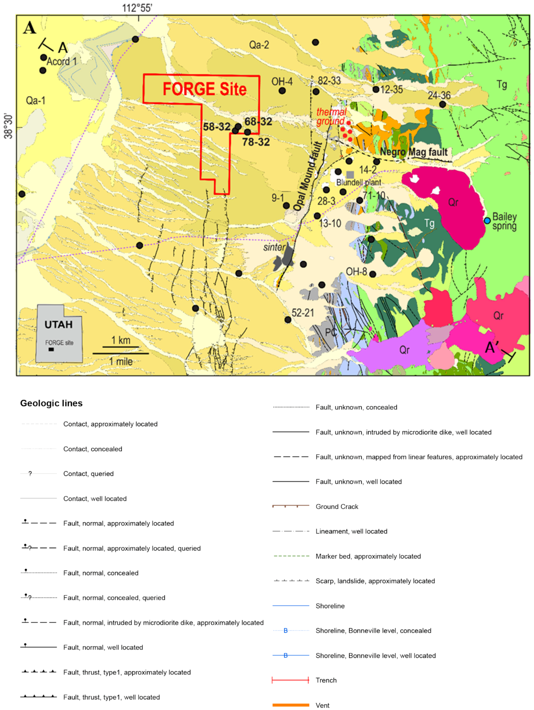
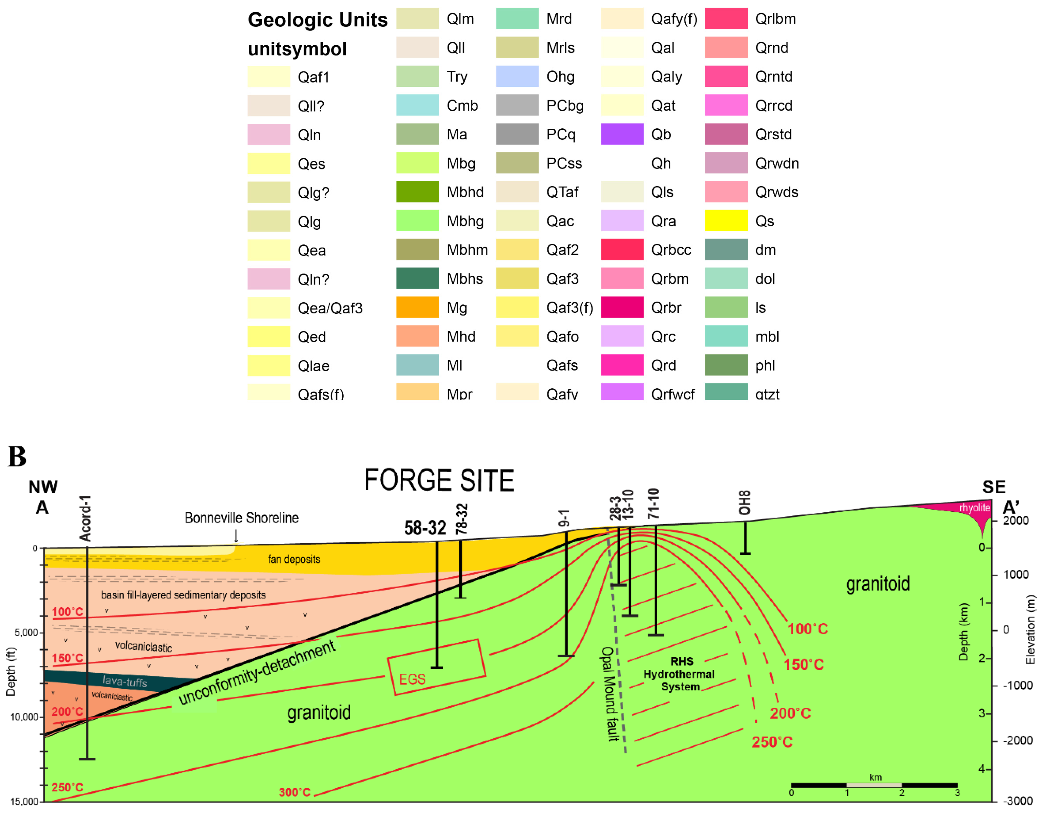
2. Geological Review of FORGE Site

The FORGE site is located ~322 km south of Salt Lake City and 16 km north of Milford, a small community with a population of 1400. The FORGE site is unpopulated and covers an area of about 5 km².

The FORGE EGS reservoir will be created in Tertiary plutonic rocks that extend westward from the core of the Mineral Mountains. The pluton is composed of diorite, granodiorite, quartz monzonite, syenite, and granite [9] (Figure 1 ranging in age from 25.4 Ma [10] to 8 Ma [9,11]. In this paper, the plutonic rocks are collectively referred to as granitoid. Quaternary (0.5–0.8 Ma) rhyolite lava flows originating from domes along the crest of the Mineral Mountains partially cover the Precambrian gneiss exposed along the flank of the Mineral Mountains and the granitoid. The Paleozoic and Mesozoic sedimentary sequences dipping to the east are exposed in the northern and southern parts of the Mineral Mountains but were not encountered in any of the deep wells. Temperatures of 250 °C in the Roosevelt Hot Springs reservoir suggest the presence of a still-cooling magma chamber in the shallow crust.

As part of the FORGE program, three new vertical wells have been drilled to date. The deepest is Well 58-32. This well was drilled to a total depth (TD) of 2297 m and plugged back to 2294 m measured depth (MD) relative to the rotary Kelly bushing (RKB). All depths were reported as 7 m above ground level (GL) to be consistent with the RKB in the September 2017 injection program. Well 58-32 penetrated alluvium to a depth of 968 m RKB and a thin, sheared rhyolite dike from 968 to 974 m RKB before encountering the granitoid basement. The poorly sorted alluvial deposits are derived from the granitoid exposed to the east in the Mineral Mountains. Few fractures are visible in the Formation MicroScanner Image (FMI) log from Well 58-32 and, in thin sections, no evidence of contact metamorphism is observed. In contrast, the rhyolite and the upper ~100 m of the granitoid are extensively sheared, fractured, and locally brecciated [12].

Structural discontinuities in the Mineral Mountains and adjacent basin primarily reflect the effects of ongoing east-west Basin and Range extension that produced steeply dipping basin-bounding faults during the last ~17 Ma (e.g., [13,14]). In contrast to other parts of the Basin and Range Province, there is no surficial indication of an active high-angle range front fault east of the FORGE site or geophysical evidence of steeply dipping faults that displace the granitoid-basin fill contact.

Seismic reflection and gravity data [17,18] indicate the contact between the basin fill and the basement dips approximately 20° to 35° to the west on the east side of Milford Valley. This contact is interpreted to represent the eroded foot wall side of a steeply dipping basin-bounding fault that was tilted eastward during uplift and exhumation of the Mineral Mountains block [19,20,21]. Beneath the FORGE site, the surface was covered by alluvial deposits. The absence of recent tectonic activity along the range front is significant, because it suggests the shallow, eastern portion of the basin-forming fault is no longer active [21]. Thus, the rotated fault is not expected to influence the development and growth of the FORGE EGS reservoir.

The most prominent of the younger Basin and Range structures is the Opal Mound fault (Figure 1). Temperature and pressure data demonstrate that the Opal Mound fault forms a hydraulic barrier separating the convective, permeable Roosevelt Hot Springs geothermal system from the low-permeability thermal regime to the west, beneath the FORGE site. Faults south of the FORGE site form short, narrow grabens and horsts [9,22] that die out as the FORGE site is approached. Three-dimensional seismic reflection surveys confirmed the shallow nature of these faults [18] and the absence of any fault offsets in the granitoid-alluvial contact greater than a few 10 s of meters.

The Negro Mag fault trends east-west (Figure 1). The fault cuts across the Mineral Mountains for ~6 km. An east-west-trending structure, 2 km south of the Negro Mag fault, was the site of seismicity recorded in the late 1970s [9,23]. Both the Negro Mag and Opal Mound faults appear to terminate at their intersection.

Despite the Mineral Mountain rotation, the current extensional regime enables an assessment of the vertical and horizontal principal stress directions. At the FORGE site, the orientation of the maximum total horizontal stress, ${\sigma }_{Hmax}$, was inferred from the Well 58-32 FMI log. More than 2000 natural fractures and 356 induced fractures were identified during logging in 2017 before running production casing [24] (Figure 2). Azimuths of the induced fractures indicate the orientation of ${\sigma }_{Hmax}$ trends NNE-SSW (Figure 2). The same fractures were mapped in an FMI log run in the openhole section of Well 58-32 after the 2019 stimulation. Similar orientations were recorded from televiewer logs run in wells 14-2 and 52-21 ([25]; Davatzes, 2016, written comm.) (refer to Figure 1). The consistency of stress orientations in the wells indicates that the direction of ${\sigma }_{Hmax}$ is consistent across the region.

A comparison of the pre- and poststimulation FMI logs from September 2017 demonstrates that significant enhancement and growth of the induced fractures occurred during injection testing (Figure 3). The orientations of these enhanced fractures confirm the NNE-SSW orientation of ${\sigma }_{Hmax}$.

3. Injection Activities

Well 58-32 is a pilot well for testing and monitoring at the FORGE site. This well was drilled to a total depth of 2297 m RKB and penetrated more than 1300 m of granitoid. After completion, 46 m of openhole was left below the production casing shoe. The well encountered low-permeability crystalline rocks at 968 m RKB. A static bottomhole temperature of 199 °C was measured at total depth. In September 2017, an initial injection program was carried out in the openhole section at the toe. A follow-on injection program was carried out in this same well in April and May 2019. The 2019 program repeated the injection into the openhole section (Zone 1) and pumped into two cased and perforated zones farther uphole (denoted as Zone 2 and Zone 3; see below). The zones were isolated during testing with packers and bridge plugs.

The zones are as follows and depicted in Figure 4:

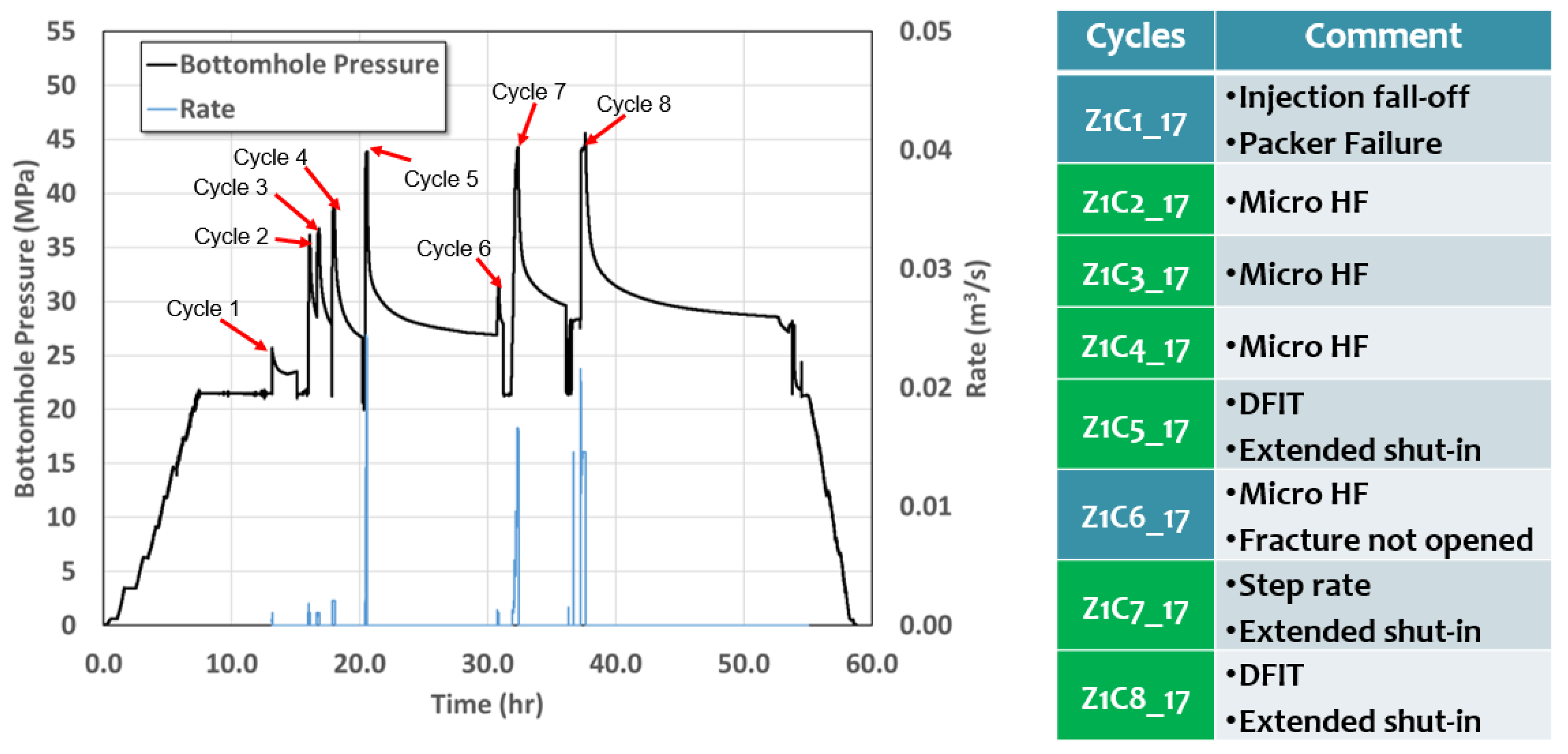
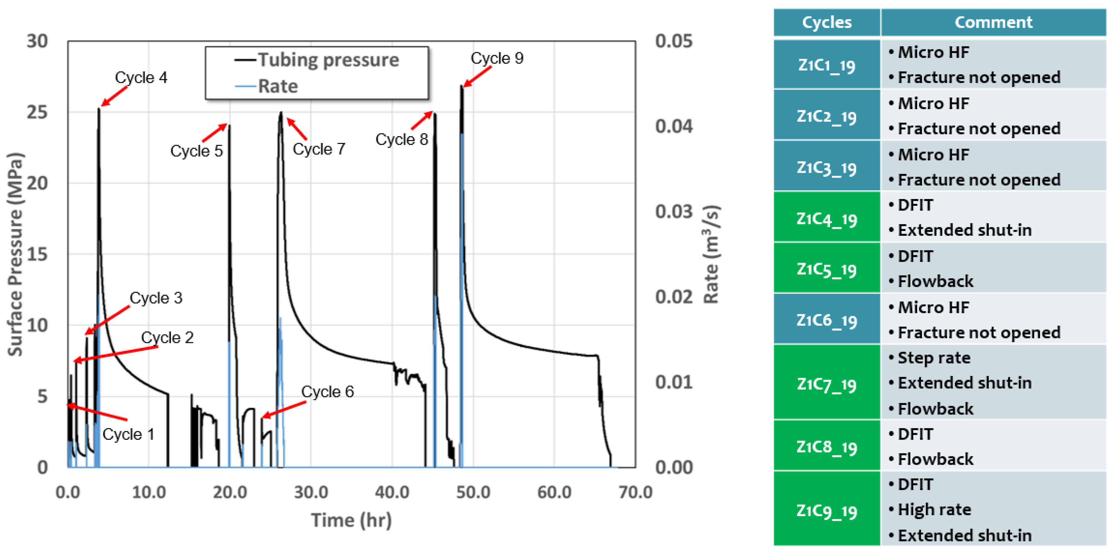
• Zone 1 is the barefoot section of the hole, extending from the production shoe at 2248 m MD to the plug back total depth at 2294 m MD. For this zone, all gradient calculations were carried out at a depth of 2262 m true vertical depth (TVD), relative to the RKB. This zone was previously stimulated in Sept. 2017 at rates up to $2.3\times {10}^{-2}$ m³/s. During the 2019 testing program, injection rates as high as $3.9\times {10}^{-2}$ m³/s were implemented.
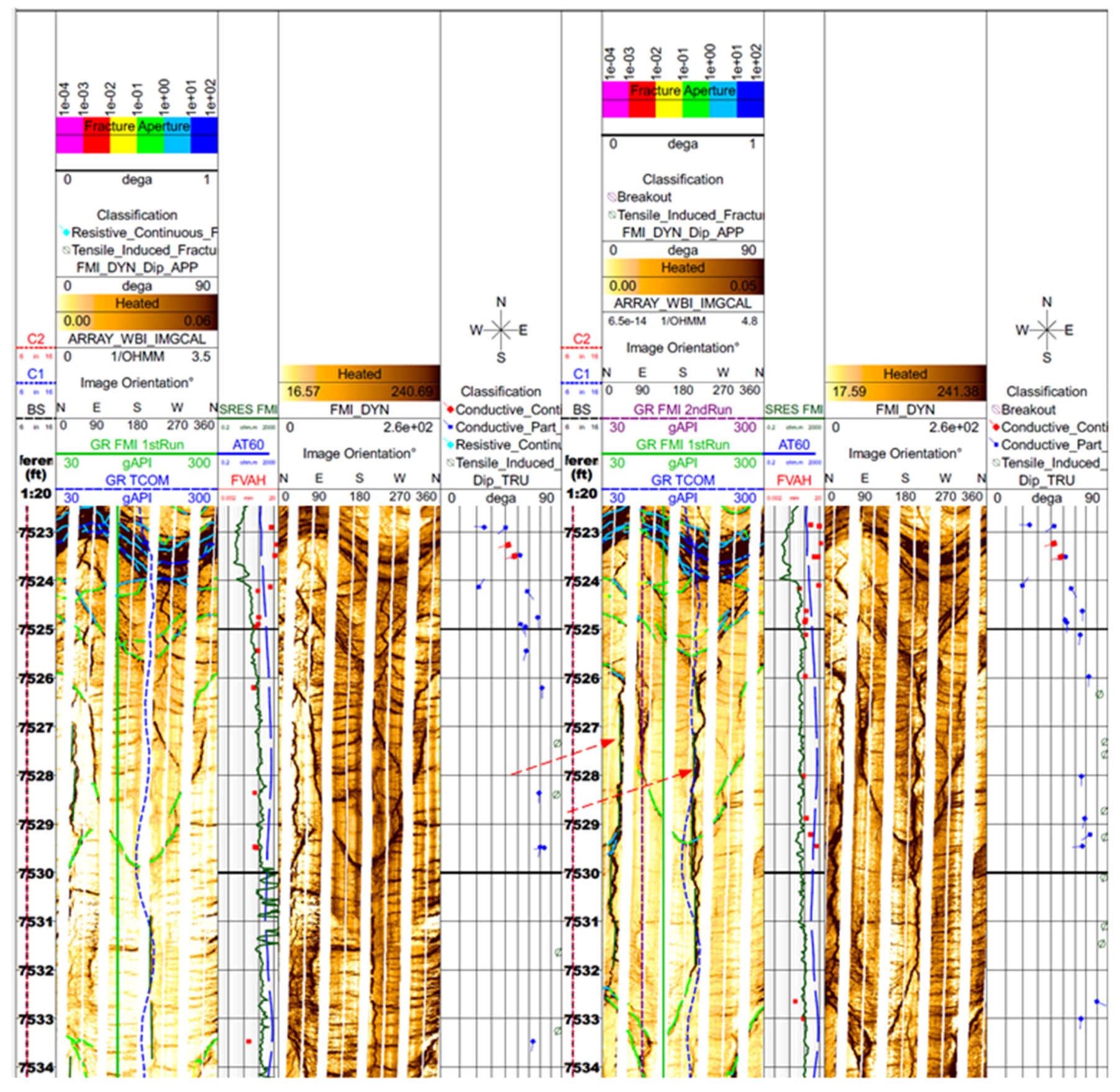
• Zone 2 was perforated over a 3-m interval from 2123 to 2126 m MD. The guns were loaded with 30-g charges at six shots per foot and 60° phasing. Gradients were calculated using a depth of 2122 m TVD RKB September 2017. This zone was picked, because it contained abundant pre-existing fractures (determined from an FMI log run before casing in 2017) that were anticipated to be near critically stressed and prone to shear and dilation.
• Zone 3 was perforated over a 3-m interval from 2001 to 2004 m MD. The guns were fired at six shots per foot with 30-g charges and 60° phasing. Gradients were calculated at a depth of 2000 m TVD RKB September 2017. This zone contained few fractures that were not prone to shear and dilation. The stimulation of Zone 3 was interrupted by the failure of the bridge plug. The consequent anticipation was that breakdown would be difficult (before the failure of the isolation tools). This proved to be true.

In each zone, a program of up to nine injection cycles was conducted. Zone 1 was treated twice—in 2017 and again in 2019. These injection activities included pump-in/shut-in, pump-in/flowback, step rate tests, and combinations. During the 2019 injection, all the bottomhole pressure and temperature information failed. Figure 5, Figure 6 and Figure 7 depict the entire chronology (pressure and pumping rate data) in Zones 1 and 2. Zone 3 was not broken down, despite pressurization to the limit of the allowable system pressure (44.8 MPa at the surface). The bridge plug failed in Zone 3 after Cycle 6.

4. In-Situ Stress Interpretation from Step Rate and Pump-In/Shut-In Tests

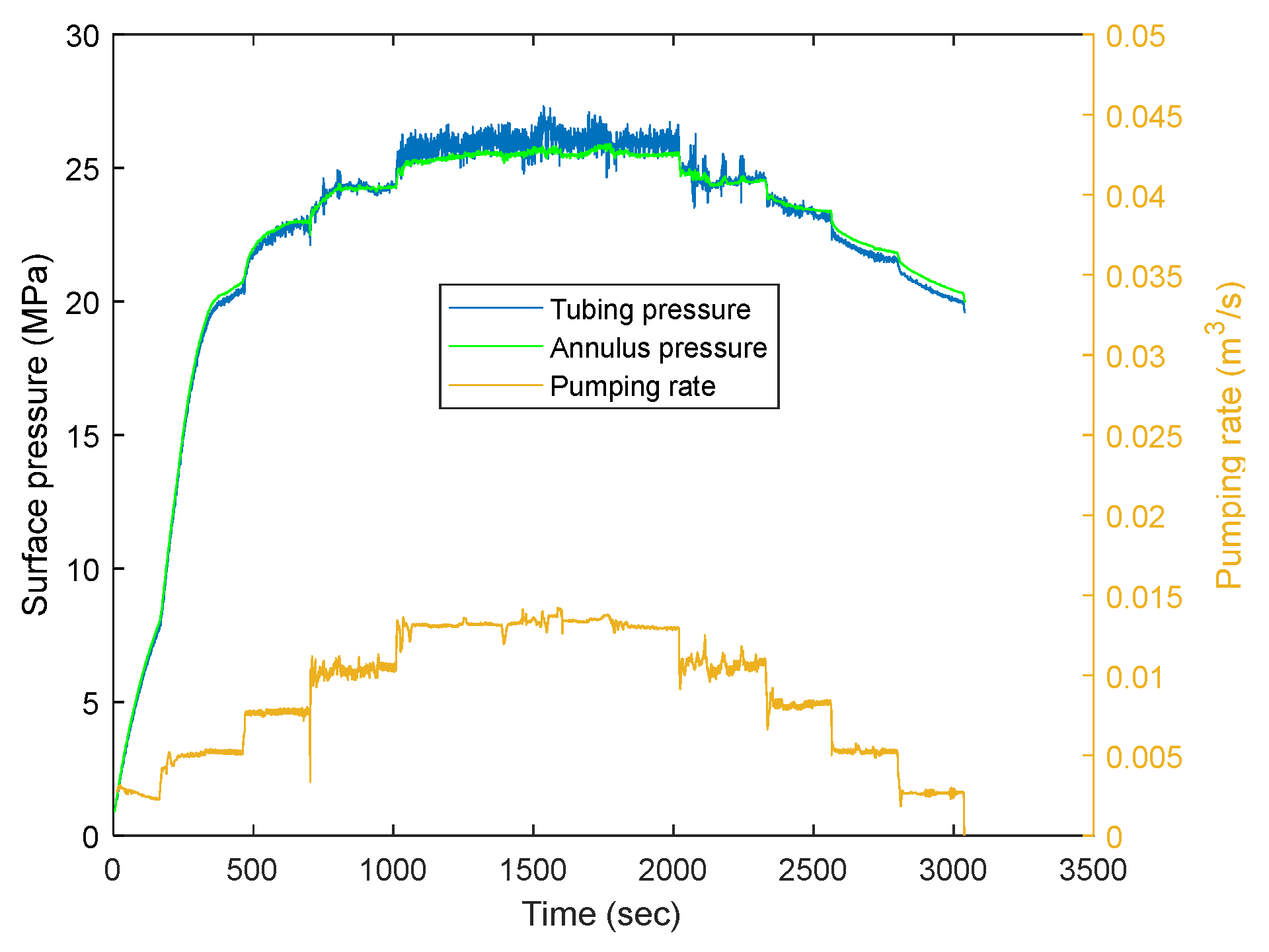
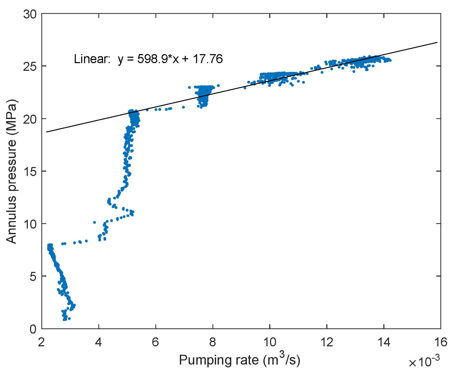
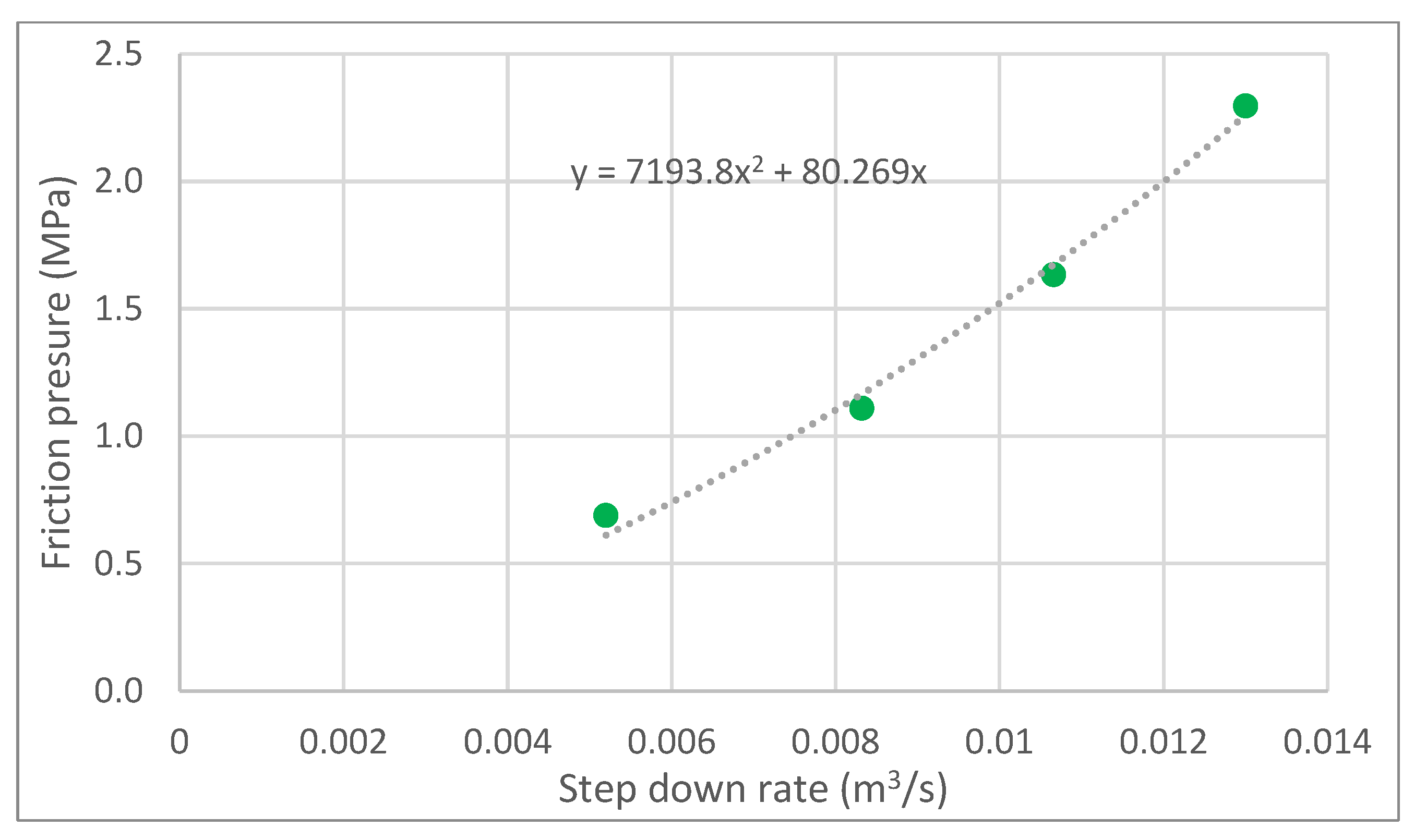
4.1. In-Situ Stress Inferred from Step Rate Tests and Estimation of Near-Wellbore Friction

Step rate tests can be used to infer the in-situ stress, and step down tests can be employed to obtain near-wellbore tortuosity and perforation friction where appropriate. Step rate tests were conducted in both Zone 1 and Zone 2 (refer to Figure 5, Figure 6 and Figure 7).

Cycle 7 of Zone 1 during the 2019 injection provided an example of step rate tests. This zone was not cased. Figure 8 illustrates the pumping rate and surface pressure for this cycle. The downhole gauges failed during the 2019 injection, and hence, no bottomhole pressure was recorded. Figure 9 shows the annulus pressure vs. the pumping rate during the increasing rate stage. The packer above the perforated zone had failed, and the annulus was exposed to pressure. This is a classic “dead string” configuration. Since there is no friction in the annulus, adding the hydrostatic pressure to the annulus pressure measured at the surface is a reliable measure of the bottomhole pressure. As shown in Figure 9 for the step rate test with increasing rate, the fracture closure pressure is the intercept of the upper linear section of the surface annulus pressure, which is estimated as 17.8 MPa. We can obtain the fracture closure pressure from the step rate down test using a similar procedure. As indicated, the annulus pressure is used, because it does not include tubing friction. The corresponding bottomhole pressure can be calculated as:

$$p_{BH}=p_{sf}+p_{hydro}=p_{sf}+{\lambda }_p{h}_{TVD}$$

(1)

where $p_{BH}$ is the bottomhole pressure, $p_{sf}$ is the surface annulus pressure, $p_{hydro}$ is the hydrostatic pressure, ${\lambda }_p$ is the hydrostatic gradient (9.8 MPa/km taken as constant all throughout the study), and $h_{TVD}$ is the TVD. TVD in Zone 1 ($h_{TVD}$) is 2262 m. Hence, in Zone 1, Cycle 7 during 2019 injection, the inferred closure stress is 39.9 MPa, and the closure stress gradient is 17.6 MPa/km.

While using the annulus pressure eliminates considering tubing friction, it is still desirable to consider the near-wellbore losses due to the perforations and tortuosity. Figure 10 plots the “friction” pressure change with the step-down pumping rate. Incremental friction pressure is the instantaneous pressure drop when the pumping rate is decreased, which can be calculated as the pressure difference between the end of the previous rate and the beginning of the current rate. Since annulus pressure is used, tubing friction is excluded, and the friction obtained from Figure 10 is exclusively near-wellbore friction. This near-wellbore friction can be then treated as tortuosity, since there are no perforations in the openhole section. Then, we can apply the near-wellbore friction correction obtained from this cycle to the closure pressure estimation of other cycles in Zone 1 (the openhole section) during the 2019 injection. This simple demonstration is a reminder that near-wellbore losses may be somewhat akin to entrance losses in pipe flow and are not insignificant.

4.2. Closure Stress Inferred from Pump-In/Shut-In Tests

Most of the injection tests in Well 58-32 are pump-in/shut-in tests, including microhydraulic fracture tests and Diagnostic Fracture Injection Tests (DFIT). The differences between a microhydraulic fracture test and a DFIT are that the former uses a much lower pumping rate and pumping volume. In this testing program, microhydraulic fracture tests are characterized by pumping rates of $1.0\times {10}^{-3}–5.2\times {10}^{-3}$ m³/s and pumping volumes of 0.1–1.6 m³, while DFITs are characterized by pumping rates of $1.3\times {10}^{-2}–3.9\times {10}^{-2}$ m³/s and pumping volumes of 4.5–30.2 m³.

Various methods were used to infer the closure stress from pump-in/shut-in tests. Several methods—including G function analysis, plotting pressure vs. $\sqrt{t}$, and diagnostic log-log plots—can be used to infer the closure stress by processing the falloff pressure during an extended shut-in. The description of these methods is as follows:

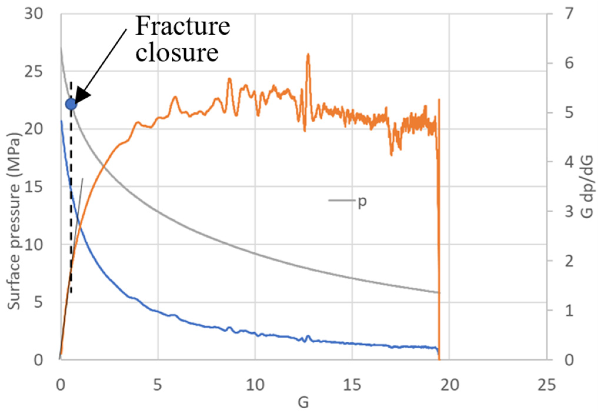
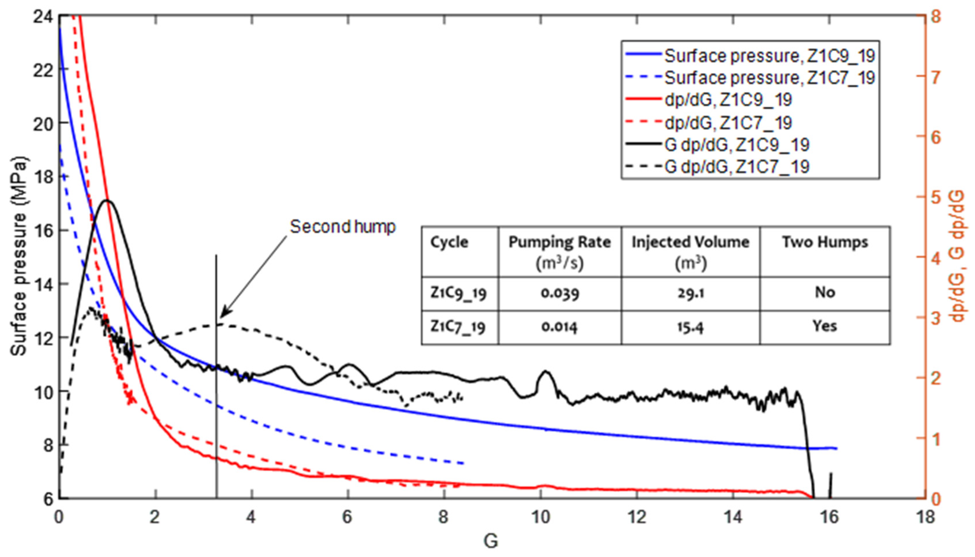
• The first method, G-function analysis, uses a superposition time, known as the G-function. This is the most commonly used method in hydrocarbon settings. This superposition time is a modified version of the time since shut-in and the injection time. Origins for the G-function derive from methods developed to calculate leak-off coefficients during hydraulic fracturing (see, for example, [3,26]). Economides and Nolte [27] provide a clear description of the original principles, including the basic premise of a bi-winged fracture with ad hoc modifications for complexity. For the G-function method, the fracture closure pressure is picked as an inflection point that distinguishes change on a derivative plot, dp/dG, or G dp/dG vs. G, related to the change in leak-off before and after fracture closure.
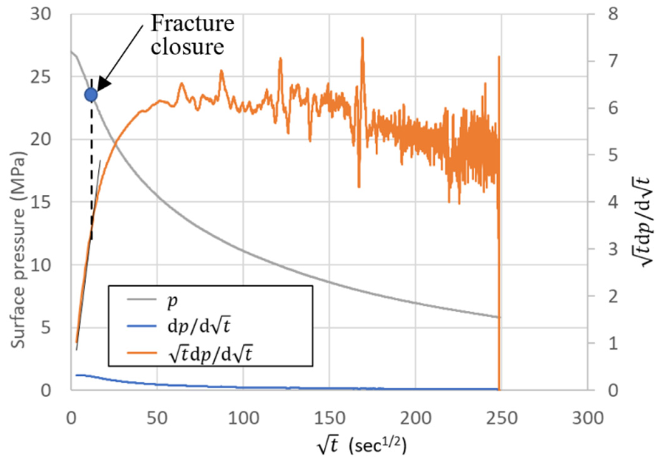
• An alternative method to G-function analysis is to plot the pressure since shut-in versus the square root of the time since shut-in ($p \mathrm{vs}. \sqrt{t}$). A straight-line section of data is indicative of linear (fracture) flow, and the end of linearity suggests that the fracture has closed and that the pressure in the fracture is equal to the stress-causing closure.
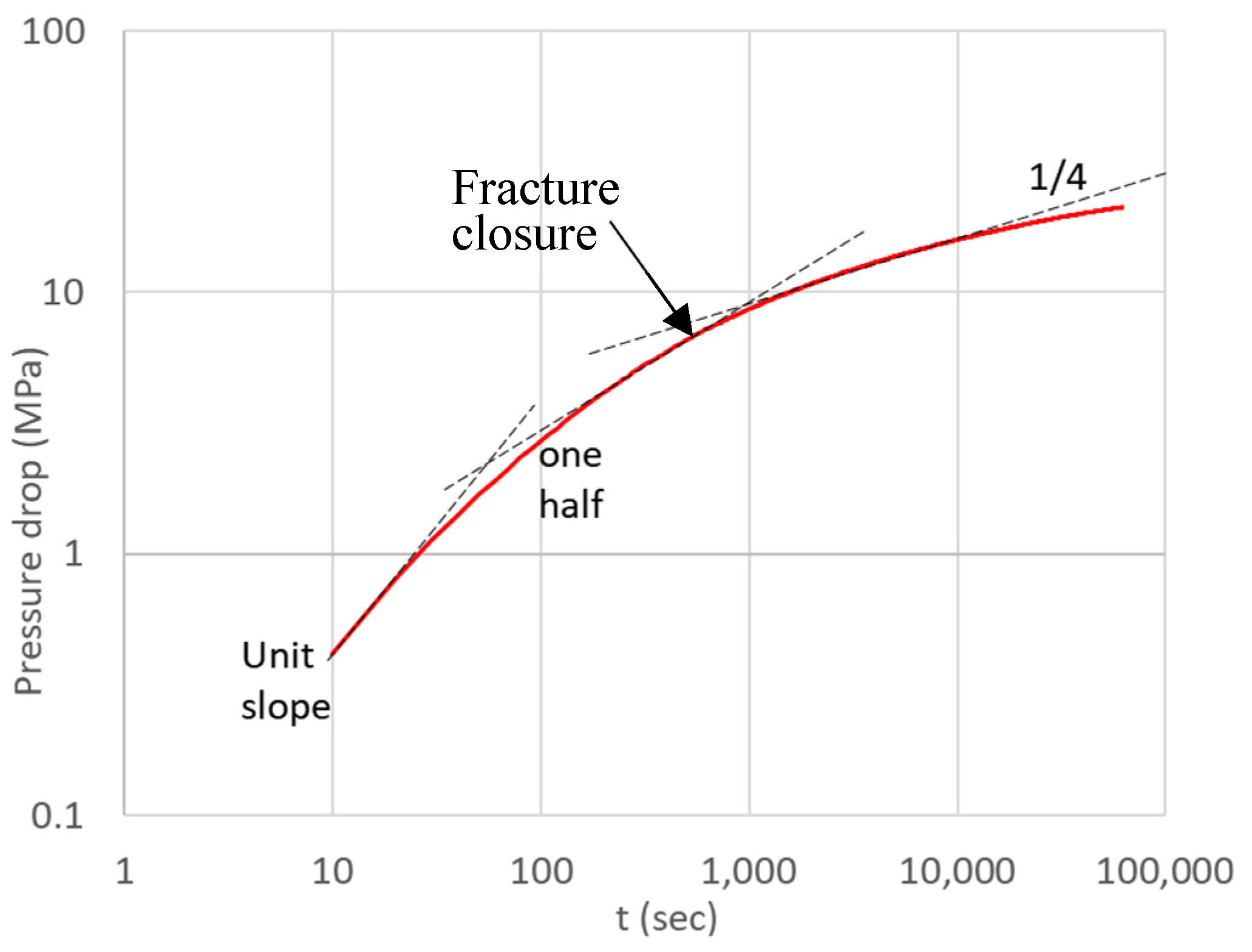
• A diagnostic log-log plot is a plot of the pressure drop since shut-in versus the time since shut-in. A one-half slope on a diagnostic plot may suggest linear flow in this single fracture (presuming a low permeability matrix). When the fracture closes, linear flow along the fracture (in this low permeability reservoir) terminates, because there is no longer adequate fracture width for effective linear flow. The pressure when linear flow ends (end of the one-half slope) is indicative of the normal stress that has closed the fracture.

Other inferences used the ISIP (instantaneous shut-in pressure) and the reopening pressure. ISIP approximates the fracture closure pressure when the near-wellbore friction is subtle, such as in some lower rate (pumping rate less than 0.002 m³/s) cycles in openhole section Zone 1. Additionally, the reopening pressure can be used to infer the fracture closure pressure by subtracting tubing friction and near-wellbore friction. The tubing friction may already be excluded by using the surface annulus pressure or the bottomhole pressure, and the near-wellbore friction can be obtained from a step rate down test (see Figure 10).

Zone 2 Cycle 8 is an example of the stress interpretation from pump-in/shut-in tests. Figure 11 shows the surface pressure and pumping rate for Zone 2 Cycle 8. This was another instance where a packer failed, and the surface annulus pressure plus the hydrostatic pressure gave the bottomhole injection pressure. We compared the closure stresses obtained by different methods for this cycle. First, we used the reopening pressure to infer the closure stress. The surface annulus pressure at reopening was 23.7 MPa. According to Equation (1), the calculated bottomhole pressure was 44.5 MPa (TVD was 2122 m for Zone 2). However, to use the reopening pressure to estimate the closure stress, it was necessary to correct this by the near-wellbore friction, including, in this case, perforation friction and tortuosity. Fortunately, there is step-down data from an earlier cycle in this zone. The near-wellbore friction estimated from the step-down test performed in Zone 2 Cycle 7 for a pumping rate of $2.1\times {10}^{-2}$ m³/s (the rate used in Zone 2 Cycle 8) is 2.8 MPa. After correction, the closure stress is 41.7 MPa, and the closure stress gradient is 19.7 MPa/km.

Picking the reopening pressure is only one method to estimate the closure stress for this cycle. We also provide the stress interpretations from other methods, which infer the closure stress from processing the falloff pressure during the extended shut-in. Figure 12, Figure 13 and Figure 14 show the closure stress interpretation from an extended shut-in period, including G-function analysis (Figure 12), analysis of pressure vs. $\sqrt{t}$ (Figure 13), and a conventional diagnostic plot (Figure 14). These techniques show the closure pressure as 42.8, 44.9, and 41.9 MPa, and the closure stress gradient as 20.1, 21.3, and 19.7 MPa/km, respectively. All values are largely in agreement.

4.3. Summary of Inferred Closure Stress from Step Rate and Pump-In/Shut-In Tests

Figure 15 summarizes the stress interpretation for the openhole zone tested in 2017 and the openhole and perforated Zone 2 in the 2019 injections. The in-situ stresses inferred by different methods for each cycle are also listed in Appendix A. Not every cycle is valid for closure stress interpretation. In some cases, such as some low injection rate/volume cycles, the fractures may not have opened or reopened. The details of the evaluation of each cycle are provided in [28,29,30].

A range of gradients is suggested in Figure 15. Some of those gradients may not be representative of the minimum in-situ stress. Possible factors affecting the gradients include near-wellbore features and/or losses, self-induced porothermoelastic back stress in a fractured environment, and dilation/contraction of fractures not aligned with the maximum horizontal total principal stress. The key observations are as follows.

(1)

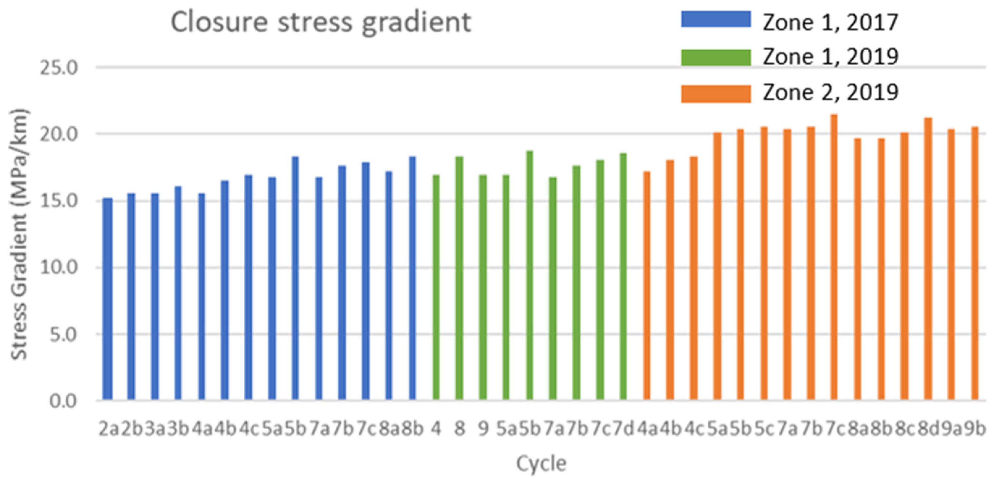
The closure stress gradients are: 15.2–18.3 MPa/km in Zone 1 2017, 16.7–18.8 MPa/km in Zone 1 2019, and 17.2–21.5 MPa/km in Zone 2. There is no stress interpretation in Zone 3, since this zone could not be broken down because of wellhead pressure limitations.

(2)

For Zone 1, the in-situ stress predictions from the 2019 injection are consistent with those from the 2017 injection program, excluding the cycles with lower injection rates in 2017.

(3)

The inferred “apparent” stress gradients in Zone 2 are greater than those in Zone 1.

(4)

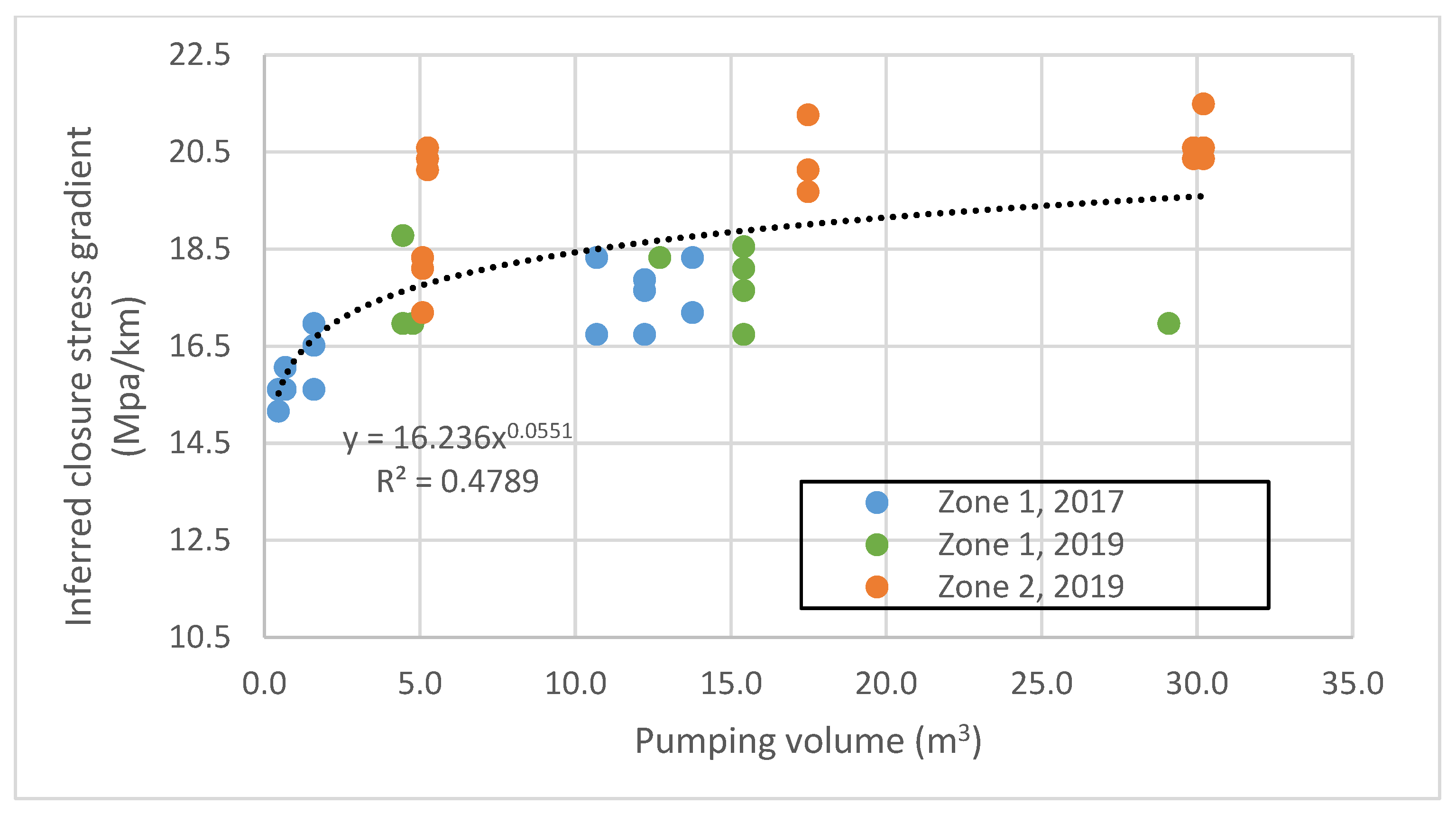
A higher pumping rate/volume gives higher closure stress.

While these are the basic results, Section 5 considers some of the anomalies, uncertainties, and unexpected observations. Some (such as intricacies of G-function interpretation or using flowback) are of interest to technologists. Other observations such as rate and volume dependence are relevant to treatment in naturally fractured formations in general.

5. Discussion

5.1. “Multiple Humps” in G-Function Plot

In some DFIT cycles, there are two humps in the GdP/dG curve in the G-function plot (e.g., Zone 1 Cycle 5 in 2017 and Zone 1 Cycle 7 in 2019), while, in other DFIT cycles, there are no such features (for example, Zone 1 Cycle 8 in 2017 and Zone 1 Cycle 9 in 2019). Figure 16 compares one cycle with two humps (Zone 1 Cycle 7 in 2019) and another cycle without two humps (Zone 1 Cycle 9 in 2019).

Nadimi et al. [31] suggested multiple humps may represent the closure of different sets of fractures. In their assumption, the first hump could be the indication of the closure of a secondary set of fractures not perpendicular to ${\sigma }_{hmin}$ while the second hump is the signature of the primary fracture set perpendicular to ${\sigma }_{hmin}$. In contrast, Liu and Ehlig-Economides [32] interpret a first hump as the initial contact and a second hump as the hydraulic fracture closure. This also opens the possibility of the second peak being an analytical artifact.

5.2. Effect of Pumping Rate and Pumping Volume

The inferred closure stresses show a correlation with the pumped volume. Figure 17 shows inferred closure stress increases with the pumped volume for both Zone 1 and Zone 2. As more fluid is injected into the reservoir, there will be greater “back stress” applied against the hydraulic fracture, resulting in higher closure stress. The cycles with a similar pumping volume in Zone 1 during 2017 and Zone 1 during 2019 yield similar inferred closure stresses. However, the inferred closure stresses for cycles in Zone 2 are higher than those of Zone 1, despite similar pumping volumes.

5.3. Effect of Previous Injection on the Current Cycle

In addition to the influence of pumping volume, a more definitive trend was that the previous injection cycle impacted the closure pressure in the following injection cycle. Figure 18 compares two cycles in sequence, Cycle 4 and Cycle 5 in Zone 2. Cycle 4 is the first DFIT cycle in Zone 2 where breakdown occurred, as is dramatically evident in the figure. Cycle 5 is a DFIT immediately following Cycle 4. The pumping rate and pumping volume for these two cycles are the same. However, the annulus pressure of Cycle 5 is about 1.4–2.1 MPa higher than that of Cycle 4 after breakdown. The higher pressure in Cycle 5 could be due to accessing a network of adjacent fractures that resulted from the slippage and dilation of natural fractures in Cycle 4. From Figure 15, we can also see that all the inferred closure stresses after Cycle 4 are greater than those of Cycle 4. The reason could be that Cycle 4 caused the natural fracture to slip and dilate, and hence, the total stress in the region of injection increased. Therefore, the subsequent injection cycles had higher treatment pressure and fracture closure pressure.

5.4. Role of Natural Fractures

Natural fractures likely played an important role in the in-situ stress measurements. While this is a thermally conductive regime, there are abundant healed and partially healed natural fractures [33]. There are four basic observations. First, at least some of the natural fractures are hydraulically conducive and could participate in hydraulic fracture initiation. Even if they are poorly conductive, they could lead to reopening in a plane that is not normal to the minimum principal stress. Zone 2, with relatively abundant natural fractures, was successfully treated with hydraulic fracturing, while Zone 3, with few natural fractures, was largely unaffected. Secondly, the inferred closure stress increased with the pumping rate/volume. This is reminiscent of a “back stress” caused by poroelasticity in an equivalent porous medium (the fractures providing the porosity). The natural fracture network will enhance the poroelasticity effect and make the “back stress” greater. Thirdly, the closure stress increased in the later cycles, which was related to more natural fractures being pressurized away from the dominant fracture network due to the previous treatment. The dilation and slippage of natural fractures made the total stress of the injection region greater. Finally, diverse/discrete natural fracture networks may have contributed to the higher closure stress gradients in Zone 2. If the natural fractures are connected to the wellbore and are not perpendicular to ${\sigma }_{hmin}$, the hydraulic fracture would propagate—at least initially—along the natural fractures, resulting in a higher closure pressure.

5.5. Alternative Interpretation Techniques

As is shown, the inferred closure stress is different in Zone 1 and Zone 2; the closure stress increases with the pumping volume and may increase from cycle to cycle. There are still uncertainties in the actual interpretation of the closure stress magnitude. Therefore, other techniques, rather than the traditional methods, might provide another perspective on closure stress.

The first alternative technique is to interpret closure stress from the pump-in/flowback tests. Flowback measurements are a desirable substitute for measurements that require unreasonably long shut-in periods as part of a DFIT. Xing et al. [7,34] provided a detailed analysis of the flowback tests at the FORGE site. The estimated closure stress for Zone 2 determined from flowback tests is 14.7–15.4 MPa/km, which is much lower than the values of 17.2–21.5 MPa/km estimated from step rate and extended shut-in tests. This could suggest that: (1) when analyzing flowback data, an artificial gradient is being picked, since the flowback started after the fractures began to close, or (2) flowback offers a very useful method for closure stress interpretation in naturally fractured reservoirs where there is poorly developed or tortuous communication between the wellbore and a natural fracture system. The pump-in/flowback method minimizes the effects of natural fractures, because the flowback rate is much larger than after shut-in leak-off and has a much stronger signature. Pump-in/flowback methods reduce the measurement time and could give better estimation in a reservoir with natural fracture networks.

Another alternative in-situ stress assessment technique is to interpret stress from the bottomhole temperature. Xing et al. [8] forecast in-situ stress using temperature signatures. The closure stresses obtained from temperature interpretation for Zone 1, 2017 range from 14.9–17.9 MPa/km, which is close to those inferred from step rate tests and extended shut-in tests, 15.2–18.3 MPa/km. The advantage of closure stress interpretation with bottomhole temperature is that the temperature signature of fracture closure is easily distinguishable, and the selection is unambiguous.

6. Conclusions

Closure stress interpretations are presented for the injection activities in FORGE Well 58-32. Step rate tests and extended shut-in tests were interpreted with various methods. There are differences in closure stresses between the openhole zone (Zone 1) tested in 2017 and again in 2019 and a newly stimulated zone behind casing (Zone 2). The inferred closure stresses of Zone 2 (17.2–21.5 MPa/km) are significantly higher than those of Zone 1 (15.2–18.3 MPa/km). The higher stress gradient in Zone 2 could be caused by the near-wellbore tortuosity, and the generated or the mobilized fracture may not be perpendicular to ${\sigma }_{hmin}$. There could also be natural variations in the stresses existing in the granitoid where the measurements were carried out.

The closure stress increases with the pumping volume and is larger in later cycles than in earlier treatments. This is attributed to an equivalent poroelastic effect and the dilation and slippage of the natural fractures.

The natural fractures within the FORGE reservoir likely played an important role in the in-situ stress measurements. The natural fractures participated in hydraulic fracture initiation, generated greater “back stress” (surrogate poroelastic effect), increased the local total stress due to slippage and dilation, and contributed to higher closure stress in Zone 2 if they were connected to the wellbore and not perpendicular to ${\sigma }_{hmin}$.

In addition to the step rate and pump-in/extended shut-in tests, pump-in/flowback data and bottomhole temperature signatures can be used to interpret the in-situ stress measurements. The inferred closure stresses from pump-in/flowback tests for Zone 2 are lower than those from step rate and extended shut-in tests. Stresses determined from temperature signatures for Zone 1, 2017 gives results that are similar to the standard interpretations. These alternative methods are valuable references and can crosscheck the predictions determined from the step rate and extended shut-in tests.

References

1. Moore, J.; McLennan, J.; Allis, R.; Pankow, K.; Simmons, S.; Podgorney, R.; Wannamaker, P.; Bartley, J.; Jones, C.; Rickard, W. The Utah Frontier Observatory for Research in Geothermal Energy (FORGE): An International Laboratory for Enhanced Geothermal System Technology Development. In Proceedings of the 44th Workshop on Geothermal Reservoir Engineering, Stanford University, Stanford, CA, USA, 11–13 February 2019. [Google Scholar]
2. Haimson, B.; Cornet, F. ISRM Suggested Methods for rock stress estimation—Part 3: Hydraulic fracturing (HF) and/or hydraulic testing of pre-existing fractures (HTPF). Int. J. Rock Mech. Min. Sci. 2003, 40, 1011–1020. [Google Scholar] [CrossRef]
3. Castillo, J.L. Modified Fracture Pressure Decline Analysis Including Pressure-dependent Leakoff. In Proceedings of the Low Permeability Reservoirs Symposium, Denver, CO, USA, 18–19 May 1987. Paper SPE 16417. [Google Scholar]
4. Barree, R.D.; Mukherjee, H. Determination of pressure dependent leakoff and its effect on fracture geometry. In Proceedings of the SPE Annual Technical Conference and Exhibition, Denver, CO, USA, 6–9 October 1996. [Google Scholar]
5. McClure, M.; Bammidi, V.; Cipolla, C.; Cramer, D.; Martin, L.; Savitski, A.; Sobernheim, D.; Voller, K. A Collaborative Study on DFIT Interpretation: Integrating Modeling, Field Data, and Analytical Techniques. In Proceedings of the Unconventional Resources Technology Conference, Denver, CO, USA, 22–24 July 2019; Society of Exploration Geophysicists: Tulsa, OK, USA, 2019; pp. 2020–2058. [Google Scholar]
6. Hickman, S.H.; Zoback, M.D. The interpretation of hydraulic fracturing pressure-time data for in-situ stress determination. In Workshop on Hydraulic Fracturing Stress Measurements; U.S. National Committee for Rock Mechanics, National Academy Press: Washington, DC, USA, 1983; pp. 44–54. [Google Scholar]
7. Xing, P.; Goncharov, A.; Winkler, D.; Rickard, B.; Barker, B.; Finnila, A.; Ghassemi, A.; Podgorney, R.; Moore, J.; Mclennan, J. Flowback Data Evaluation at FORGE. In Proceedings of the 54th US Rock Mechanics/Geomechanics Symposium, Golden, CO, USA, 28 June–1 July 2020. [Google Scholar]
8. Xing, P.; McLennan, J.; Moore, J. In-situ Stress Measurement Using Temperature Signatures. 2020; in preparation. [Google Scholar]
9. Nielson, D.L.; Evans, S.H.; Sibbett, B.S. Magmatic, structural, and hydrothermal evolution of the Mineral Mountains intrusive complex, Utah. Geol. Soc. Am. Bull. 1986, 97, 765–777. [Google Scholar] [CrossRef]
10. Aleinikoff, J.N.; Nielson, D.L.; Hedge, C.E. Mineral mountains, South-Central Utah. In Shorter Contributions to Isotope Research: Topical Reports on Geochronology and Isotope Geochemistry; Department of the Interior, US Geological Survey: Reston, VA, USA, 1986; p. 1. [Google Scholar]
11. Coleman, D.S.; Walker, J.D. Evidence for the generation of juvenile granitic crust during continental extension, Mineral Mountains Batholith, Utah. J. Geophys. Res. Space Phys. 1992, 97, 11011–11024. [Google Scholar] [CrossRef] [Green Version]
12. Jones, C.G.; Moore, J.N.; Simmons, S. Petrography of the Utah FORGE site and environs, Beaver County, Utah. In Geothermal Characteristics of the Roosevelt Hot Springs System and Adjacent FORGE EGS Site; Allis, R., Moore, J.N., Eds.; Utah Geological Survey Miscellaneous Publications: Milford, UT, USA, 2019; Volume 169-K, p. 23. [Google Scholar] [CrossRef]
13. Hintze, L.F.; Davis, F.D. Geology of Millard County, Utah. UGS Bull. 2003, 133, 305. [Google Scholar]
14. Dickinson, W.R. Geotectonic evolution of the Great Basin. Geosphere 2006, 2, 353. [Google Scholar] [CrossRef] [Green Version]
15. Kirby, S.M. Revised mapping of bedrock geology adjoining the Utah FORGE site. In Geothermal Characteristics of the Roosevelt Hot Springs System and Adjacent FORGE EGS Site; Allis, R., Moore, J.N., Eds.; Utah Geological Survey Miscellaneous Publications: Milford, UT, USA, 2019; Volume 169-A, p. 6. [Google Scholar] [CrossRef]
16. Kirby, S.M.; Knudsen, T.R.; Kleber, E.; Hiscock, A. Geologic setting of the Utah FORGE site, based on new and revised geologic mapping. Trans. Geotherm. Resour. Counc. 2018, 42, 1097–1114. [Google Scholar]
17. Hardwick, C.; Hurlbut, W.; Gwynn, M. Geophysical surveys of the Milford, Utah, FORGE site—Gravity and TEM. In Geothermal Characteristics of the Roosevelt Hot Springs System and Adjacent FORGE EGS Site; Allis, R., Moore, J.N., Eds.; Utah Geological Survey Miscellaneous Publications: Milford, UT, USA, 2019; Volume 169-F, p. 15. [Google Scholar] [CrossRef]
18. Miller, J.; Allis, R.; Hardwick, C. Interpretation of seismic reflection surveys near the FORGE enhanced geothermal systems site, Utah. In Geothermal Characteristics of the Roosevelt Hot Springs System and Adjacent FORGE EGS Site; Allis, R., Moore, J.N., Eds.; Utah Geological Survey Miscellaneous Publication: Milford, UT, USA, 2019; Volume 169-H, p. 13. [Google Scholar] [CrossRef]
19. Coleman, D.S.; Walker, J.D. Modes of Tilting During Extensional Core Complex Development. Science 1994, 263, 215–218. [Google Scholar] [CrossRef] [PubMed]
20. Coleman, D.S.; Bartley, J.M.; Walker, J.D.; Price, D.E.; Friedrich, A.M. Extensional faulting, footwall deformation and plutonism in the Mineral Mountains, southern Sevier desert. Brigh. Young Univ. Geol. Stud. 1997, 42, 203–233. [Google Scholar]
21. Bartley, J.M. Joint Patterns in the Mineral Mountains Intrusive Complex and Their Roles in Subsequent Deformation and Magmatism. In Geothermal Characteristics of the Roosevelt Hot Springs System and Adjacent FORGE EGS Site; Allis, R., Moore, J.N., Eds.; Utah Geological Survey Miscellaneous Publications: Milford, UT, USA, 2019; Volume 169-C, p. 13. [Google Scholar] [CrossRef]
22. Kleber, E.; Hiscock, A.; Kirby, S.; Allis, R.; Quirk, B. Assessment of Quaternary faulting near the Utah FORGE site from high resolution topographic data. Trans. Geotherm. Resour. Counc. 2017, 41, 1–2. [Google Scholar]
23. Zandt, G.; McPherson, L.; Schaff, S.; Olsen, S. Seismic Baseline and Induction Studies: Roosevelt Hot Springs, Utah and Raft River, Idaho; ID/01821-T1; U.S. Department of Energy: Washington, DC, USA, 1982.
24. Handwerger, D.A.; McLennan, J.D. Wireline log and borehole image interpretation for FORGE well 58-32, Beaver County, Utah, and integration with core data. In Geothermal Characteristics of the Roosevelt Hot Springs System and Adjacent FORGE EGS Site; Allis, R., Moore, J.N., Eds.; Utah Geological Survey Miscellaneous Publications: Milford, UT, USA, 2019; Volume 169-M. [Google Scholar] [CrossRef]
25. Keys, W.S. Borehole geophysics in igneous and metamorphic rocks. In Proceedings of the 20th Annual Symposium, Tulsa, OK, USA, 3–6 June 1979. [Google Scholar]
26. Nolte, K. Principles for Fracture Design Based on Pressure Analysis. SPE Prod. Eng. 1988, 3, 22–30. [Google Scholar] [CrossRef]
27. Economides, M.J.; Nolte, K.G. (Eds.) Reservoir Stimulation; John Wiley & Sons: Englewood Cliffs, NJ, USA, 2000. [Google Scholar]
28. Xing, P.; McLennan, J.; Moore, J. Re-evaluation of In-Situ Stress Determinations in Well 58-32. Report to U.S. Department of Energy. 2020; in preparation. [Google Scholar]
29. McLennan, J.D.; Moore, J. Utah FORGE: Phase 2C Topical Report (No. 1187), Appendix A Injection Measurements in Well 58-32 (April and May 2019); U.S. Department of Energy: Washington, DC, USA, 2019.
30. McLennan, J.D.; Moore, J. Utah FORGE: Phase 2C Topical Report (No. 1187), Appendix B Injection Measurements in Well 58-32 (September 2017); U.S. Department of Energy: Washington, DC, USA, 2019.
31. Nadimi, S.; Forbes, B.; Moore, J.; McLennan, J.D. Effect of natural fractures on determining closure pressure. J. Pet. Explor. Prod. Technol. 2019, 10, 711–728. [Google Scholar] [CrossRef] [Green Version]
32. Liu, G.; Ehlig-Economides, C. Comprehensive before-closure model and analysis for fracture calibration injection falloff test. J. Pet. Sci. Eng. 2019, 172, 911–933. [Google Scholar] [CrossRef]
33. Finnila, A.; Forbes, B.; Podgorney, R. Building and Utilizing a Discrete Fracture Network Model of the FORGE Utah Site. In Proceedings of the 44th Workshop on Geothermal Reservoir Engineering, Stanford University, Stanford, CA, USA, 11–13 February 2019. [Google Scholar]
34. Xing, P.; Winkler, D.; Rickard, B.; Barker, B.; Finnila, A.; Ghassemi, A.; Pankow, K.; Podgorney, R.; Moore, J.; Mclennan, J. Interpretation of In-Situ Injection Measurements at the FORGE Site. In Proceedings of the 45th Workshop on Geothermal Reservoir Engineering, Stanford University, Stanford, CA, USA, 10–12 February 2020. [Google Scholar]
Figure 1. (A) Geologic map of the FORGE site and surrounding area (modified from [9], the name of the publisher: Geological Society of America; and [15], the name of the publisher: Utah Geological Survey). For clarity, only a few of the many wells are shown. Abbreviations: Qa-1 = Lake Bonneville silts and sands, Qa-2 = alluvial fan deposits, Qr = Quaternary rhyolite lava and pyroclastic deposits, Tg = Tertiary granitoid, PC = Precambrian gneiss, and black filled circles = wells. (B) Northwest-southeast section through the FORGE site [16]. The Roosevelt Hot Springs (RHS) geothermal system lies east of the Opal Mound fault. Isotherms are interpreted from well measurements. The red box represents the approximate position of the FORGE enhance geothermal system (EGS) reservoir.
Energies 13 05842 g001aEnergies 13 05842 g001b
Figure 2. The orientation of the fractures during drilling over the logged interval of Well 58-32, adapted from [24], the name of the publisher: Utah Geological Survey The orientations of these fractures indicate that the maximum total horizontal stress ( σ H m a x ) trends NNE-SSW. The rose diagram shows the fracture azimuth (i.e., planar strike orientation), with the average (solid arrow) and mode (dashed arrow) of the azimuths indicated.
Energies 13 05842 g002
Figure 3. Comparison of Formation MicroScanner Image (FMI) logs before (left two tracks) and after (right two tracks) injection during 2017. Induced fractures are near-vertical and are shown by circles with azimuth trends to the right of the tracks. Blue tadpole symbols show the direction and dip of natural fractures. The arrows point to induced fractures that display the significant enhancement and growth after injection. Depths are in feet (to convert to meters, multiply by 0.3048). For each pair, the lighter leftmost panel is known as a static view, and the rightmost panel is a dynamic view. In “static normalization”, the resistivity range of the entire logged interval is partitioned into 256 color levels. “Dynamic normalization” can enhance features locally by rescaling the color intensity over a smaller interval, enabling the contrast between adjacent resistivity levels to be enhanced. The dashed lines that run the length of the images is the gamma ray from the triple combo logging run (GR_TCOM). The logging abbreviations: SRES FMI = synthetic resistivity, AT60 = array induction two-foot resistivity A60, and FVAH = hydraulic electrical fracture aperture, cube root of the cube of the fracture trace aperture summed over a given window height.
Energies 13 05842 g003
Figure 4. Injection testing zones of Well 58-32. Zones 1 and 2 were stimulated with hydraulic fracturing, including pump-in/shut-in and pump-in/flowback tests. Attempts were made to stimulate Zone 3, but the stimulation was not successful and is not discussed in this paper. The basic principles of isolation and pumping are well-described in [2].
Energies 13 05842 g004
Figure 5. Pressure-rate relationships during the 2017 injection testing of Zone 1 (Z1) during Cycles 1–8 (C1–8). The cycle designation indicates the zone, the cycle number, and the year the measurements were made. HF = hydraulic Fracture and DFIT = Diagnostic Fracture Injection Test.
Energies 13 05842 g005
Figure 6. Pressure-rate relationships during the 2019 injection testing of Zone 1 (Z1) during Cycles 1–9 (C1–9). The cycle designation indicates the zone, the cycle number, and the year the measurements were made. See Figure 5 for abbreviations.
Energies 13 05842 g006
Figure 7. Pressure-rate relationships during the 2019 injection testing of Zone 2 (Z2) during Cycles 1–9 (C1–9). The cycle designation indicates the zone, the cycle number, and the year the measurements were made. See Figure 5 for abbreviations.
Energies 13 05842 g007
Figure 8. Injection data for a step-up/step-down test in Zone 1 Cycle 7 in 2019.
Energies 13 05842 g008
Figure 9. Annulus pressure vs. pumping rate (increasing rate) for Zone 1 Cycle 7 during the 2019 injection. One estimate of the closure pressure is the intercept of the upper linear section of the surface annulus pressure, which is 17.8 MPa. The calculated bottomhole pressure is 39.9 MPa, and the inferred stress gradient is 17.6 MPa/km.
Energies 13 05842 g009
Figure 10. Friction pressure obtained from the step-down test performed in Zone 1 Cycle 7 during the 2019 injection. Annulus pressure is used, and hence, the friction pressure obtained here only reflects near-wellbore tortuosity in the openhole completion.
Energies 13 05842 g010
Figure 11. Surface pressure and pumping rate for Zone 2 Cycle 8. Left is the entire injection and shut-in pressure, while the view at right is a zoomed-in view of early time shut-in data. The apparent reopening pressure is picked from the surface annulus pressure as 23.7 MPa (bottomhole pressure 44.5 MPa). The friction pressure obtained from the step-down rate test for Zone 2 Cycle 7 is 2.8 MPa at a pumping rate of 2.1 × 10 2 m3/s. After correcting for friction, the reopening pressure is 41.7 MPa, and the closure stress gradient is 19.7 MPa/km.
Energies 13 05842 g011
Figure 12. G-function plot of Zone 2 Cycle 8. The surface pressure at closure is 22.1 MPa, using the initial tangent. The calculated bottomhole pressure at closure is 42.8 MPa, and the closure stress gradient is 20.1 MPa/km.
Energies 13 05842 g012
Figure 13. Square root of time plot for Zone 2 Cycle 8. The surface pressure at closure is 23.4 MPa. The calculated bottomhole pressure at closure is 44.9 MPa, and the closure stress gradient is 21.3 MPa/km.
Energies 13 05842 g013
Figure 14. Diagnostic plot for Zone 2 Cycle 8. The fracture closure is picked at the end of the half-slope. Hence, the surface pressure at closure is 21.1 MPa (instantaneous shut-in pressure (ISIP) 27.0 MPa minus the pressure drop of 5.9 MPa). The calculated bottomhole pressure at closure is 41.9 MPa, and the closure stress gradient is 19.7 MPa/km.
Energies 13 05842 g014
Figure 15. Summary of closure stress gradient in different zones. Zone 1 gradients range from is 15.2–18.8 MPa/km (average 17.2 MPa/km). Zone 2 gradients range from 17.2–21.5 MPa/km (average 19.9 MPa/km). With the monotonically increasing values in Zone 2, taking the average value is not necessarily reasonable, suggesting an underlying physical mechanism. Note that each cycle may have multiple interpretations by different methods labeled as a, b, c, and d, respectively (refer to Table A1, Table A2 and Table A3 for the specific method used).
Energies 13 05842 g015
Figure 16. Comparison of the G-function between Zone 1 Cycle 7 and Zone 1 Cycle 9 during the 2019 injection program. There were two humps in GdP/dG in Zone 1 Cycle 7, 2019, while no such feature is seen in Zone 1 Cycle 9, 2019.
Energies 13 05842 g016
Figure 17. Inferred closure stress vs. pumping volume.
Energies 13 05842 g017
Figure 18. Comparison of two sequential cycles, Cycle 4 and Cycle 5, for Zone 2.
Energies 13 05842 g018
Publisher’s Note: MDPI stays neutral with regard to jurisdictional claims in published maps and institutional affiliations.