Article

Experimental and Numerical Study on Proppant Transport in a Complex Fracture System

1
State Key Laboratory of Petroleum Resource and Prospecting, China University of Petroleum (Beijing), Changping, Beijing 102249, China
2
College of Petroleum Engineering, China University of Petroleum (East China), Qingdao 266580, China
3
PetroChina Oil & Gas Pipeline Control Center, Beijing 100028, China
*
Author to whom correspondence should be addressed.
Energies 2020, 13(23), 6290; https://doi.org/10.3390/en13236290
Submission received: 19 September 2020 / Revised: 11 November 2020 / Accepted: 25 November 2020 / Published: 28 November 2020
(This article belongs to the Special Issue Modelings and Analysis of Hydraulic Fracturing in Reservoirs)

Abstract

:
Slickwater fracturing can create complex fracture networks in shale. A uniform proppant distribution in the network is preferred. However, proppant transport mechanism in the fracture network is still uncertain, which restricts the optimization of sand addition schemes. In this study, slot flow experiments are conducted to analyze the proppant placement in the complex fracture system. Dense discrete phase method is used to track the particle trajectories to study the transport mechanism into the branch. The effects of the pumping rate, sand ratio, sand size, and branch angle and location are discussed in detail. Results demonstrate that: (1) under a low pumping rate or coarse proppant conditions, the dune development in the branch depends on the dune geometry in the primary fracture, and a high proportion of sand can transport into the branch; (2) using a high pumping rate or fine proppants is beneficial to the uniform placement in the fracture system; (3) sand ratio dominates the proppant placement in the branch and passing-intersection fraction of a primary fracture; (4) more proppants may settle in the near-inlet and large-angle branch due to the size limit. Decreasing the pumping rate can contribute to a uniform proppant distribution in the secondary fracture. This study provides some guidance for the optimization of proppant addition scheme in the slickwater fracturing in unconventional resources.

1. Introduction

Complex fracture geometries can be created by using slickwater fracturing in shale resources [1,2,3]. Generally, the complex geometry is regarded as a network, with the secondary fractures, usually referred to natural fractures and bedding planes, intersecting with the primary fracture [4]. To acquire a desired fracture conductivity, a large number of proppants are injected into the network to prop the primary and secondary fractures. A uniform proppant distribution in the network is preferred. In some cases, however, a limited placement area [5,6] and an uneven proppant distribution [7,8,9] are obtained, which is probably due to the narrow width and heterogeneous orientation of secondary fractures. To solve the issue above, more work is needed to reveal the proppant transport mechanism and distribution laws in the fracture network.
In laboratories, proppant transport in a single fracture is typically simulated in a slot, which is composed of two parallel Plexiglas plates [10,11,12,13]. Using water as the fracturing fluid, mixing sand at a certain volume ratio, and pumping the slurry at one end of the slot, the proppants were found to settle on the slot bottom and a sand dune was formed [10]. Many researchers have devoted their efforts to exploring the inherent relation between the dune development and factors such as flow rate [10], fluid rheology [14], proppant properties [13], fracture width [12], and fracture surface roughness [15]. Patankar et al. [16] and Wang et al. [17] even fitted correlations to predict the equilibrium dune height. As slickwater fracturing was applied widely to the stimulation of shale-gas formations, much attention was paid to the proppant transport in the complex fracture network. Similarly, proppant transport in the fracture network is performed in a configuration in which multiple slots are joined together [18,19,20,21,22,23]. There are two types of slot intersection patterns for the experimental fracture network. One is the T-shaped pattern, in which the branch slot, served as the secondary fracture, intersects orthogonally with the primary slot, taken as the primary fracture [18,20]; the other is the V-shaped pattern, in which the secondary slot intersects with the primary slot at a specified angle [19,21,22,23].
Some experiments on proppant transport and settling in complex fracture systems have been conducted. Sahai et al. [18] proposed underlying mechanisms of proppant transport into the secondary fracture using a vertical slot system with T-shaped intersections. It was found that transporting proppants into the secondary slots is dependent on the threshold fluid velocity in the primary slot. Proppants may fall from the primary slot into the secondary slot due to gravity, while they can also turn the corner at the intersection when the fluid velocity is higher than this threshold. Tong and Mohanty [19] established a vertical slot system with a V-shaped intersection. They found the equilibrium dune height in the branch is not only related to the flowing rate in the primary slot, but is also dependent on the branch angle and sand size, especially under a high rate. Alotaibi and Miskimins [20] introduced tertiary fractures into the vertical slot system, with the tertiary slot orthogonal to the secondary slot. It was discovered that proppants can transport far into the tertiary slot. Compared with the primary slot, however, there is a lag for sand to reach the secondary and tertiary slots. They also pointed out that, rather than the fluid velocity, the degree of dune development in the primary slot heavily determines the proppants into the secondary and tertiary slots. Li et al. [21] and Pan et al. [22] extended previous conclusions and formulated correlations of dune geometries using a variety of parameters such as fluid viscosity, sand concentration, and branch angle. Furthermore, Ma et al. [23] characterized slurry velocity field in the slot configuration to quantify the relationships between the governing parameters which affect proppant placement efficiency through intersections.
Besides experimental studies mentioned above, there was also a lot of work carried out by numerically simulating proppant transport in slickwater fracturing. The discrete element method coupled with computational fluid dynamics, usually referred to as DEM-CFD, is a useful tool to characterize the proppant transport trajectories. The inter-particle and particle-wall interactions are considered, with solid particles tracked individually according to Newton’s laws of motion. Using this method, Zhang et al. [24,25] studied the proppant micromechanics and transport mechanism in a single vertical fracture and traced the placement of multi-sized proppants in vertical and horizontal wells. Baldini et al. [26] evaluated the proppant transport trajectories from different injection positions to improve the perforation placement strategy. Despite the accurate characterization of particle motion, one disadvantage of this method is the high computational demands [27,28]. To avoid this drawback, some alternative methods, such as the dense discrete phase model (DDPM) [19,29] and multiphase particle-in-cell (MP-PIC) method [30,31,32], were developed to simulate the particle transport. These approaches use a force to represent the details of inter-particle and particle-wall collisions, and use the concept of parcel to contain particles [22]. This behavior significantly reduces the number of particles involved in computations, correspondingly resulting in an acceleration in simulation speed.
Although these experiments and numerical simulations provide a systematical and preliminary understanding of proppant transport in the complex fracture system, there are still some aspects requiring further improvement and exploration. Three points are presented and discussed here. Firstly, most of the previous experiments just focused on the final dune geometry (e.g., equilibrium dune height [10,11,17]) or placement area [14] in the slot, and few systematically and quantitatively characterized the dynamic evolution of a sand dune in the slot system. Secondly, the fracture length in the configuration is limited. The length of a primary fracture in a conventional slot system is generally less than 2 m (e.g., 1.22 m used by Sahai et al. [18] and 0.381 m used by Tong and Mohanty [19]), and the length of a secondary fracture is less than 1 m (e.g., 0.19 m used by Tong and Mohanty [19] and 0.9 m used by Pan et al. [22]). According to McClure [33], under this condition, finer proppants may travel out of the slot before they settle to the bottom, and a real proppant distribution may not be recorded due to an adequate transport distance. Thirdly, few experiments combined numerical simulations to analyze the experimental results, especially the proppant transport trajectories, which cannot be precisely captured through experimental techniques.
In this paper, a large-scale configuration of the complex fracture system was used to study the dune evolution in the primary and secondary fractures. Meanwhile, a DDPM model was established to track the proppant transport trajectories under the corresponding experimental conditions. This article is organized as follows. In Section 2, the experimental apparatus, material, and procedure are described in detail. In Section 3, the experimental results of proppant transport and distribution in the complex fracture system are presented and analyzed. In Section 4, the numerical model is introduced and simulation results are in combination with experimental results to clarify the proppant transport mechanism in the complex fracture system. Following that, some conclusions are given in Section 5. The conclusions obtained in this study aim to provide guidance for the optimization of the proppant addition scheme in slickwater fracturing in unconventional resources.

2. Slot Flow Experiment

2.1. Experimental Apparatus

Proppant transport in a complex fracture system was simulated in a configuration shown in Figure 1a. Details about this apparatus, including the slot dimensions and branch position deployment, are provided in Appendix A. Here, a sketch is presented in Figure 1b to introduce the main components of this configuration. Figure 1b shows that the apparatus consists of an injection system, a fracture system, and a circulation and recycling system.
The injection system includes a blender and a progressive cavity pump. The blender, with a volume of 0.6 m3, is used to prepare slurries. Three rotation blades are installed in the blender. They can stir the mixture of proppants and fracturing fluid at a specified revolving speed to obtain the slurry, with proppants suspending in the fluid. The progressive cavity pump, with a maximum rate of 65 m3/h, serves as a power source to pressurize the slurries in the blender and propel them to flow through the circular pipe into the slot system. The fracture system is the core of this apparatus. The detailed design drawing of the fracture system is presented in Figure A1 in Appendix A. As shown in Figure 1b, this system is assembled with multiple slots, and a slot consists of two parallel Plexiglass plates. The structure of a slot is shown in Figure A1a. The total height and length of one slot are 700 mm and 1100 mm, respectively. The modeled fracture for fluid flow is the transparent area surrounded by the steel frame. The modeled fracture is 1000 mm long and 600 mm high. Besides, 30 holes with a diameter of 10 mm are drilled in the middle of the modeled fracture to simulate the effect of fluid leak-off. In this study, fluid leak-off is ignored. Due to the large dimension and limited pressure tolerance of the Plexiglass plate, the periphery and middle of the plate are reinforced by cubic-shaped angle steel.
The fracture system is composed of a vertical primary fracture, three vertical secondary fractures, one horizontal secondary fracture, and one inclined secondary fracture. Figure A1b shows that the primary fracture is assembled by connecting five identical slots with flanges, while each of the secondary fractures is joined with two slots. Considering the flange length, the primary and secondary fracture are 5940 and 2200 mm long, respectively, but the heights for both of them are the same (i.e., 600 mm). Sizes of the primary and secondary fractures in this configuration are much larger than those used in previous studies [18,19,20], which guarantees an adequate transport distance. Besides, based on a real field condition [34], a gap of 5 mm between two plates is set for the primary fracture, whereas a width of 3 mm is adopted for the secondary fracture.
Positions and orientations of secondary fractures are fixed in this apparatus. Figure A1b shows that a vertical secondary fracture with 30°-branch and 150°-branch intersects with the primary fracture at L = 1160 mm. A vertical secondary fracture with 45°-branch and 135°-branch crosses the primary fracture at L = 2430 mm. Following that, a vertical secondary fracture with two 90°-branches intersects with the primary fracture at L = 3640 mm. The horizontal and inclined branches are placed at slots 4 and 5, respectively. The case in which a natural fracture intersects with the primary fracture was considered in this paper. Hence, one of the first three vertical secondary fractures, along with the primary fracture, is used to form the experimental fracture system.
The circulation and recycling system includes magnetic flow meters, valves, and a sedimentation pool. Magnetic flow meters are installed near the inlet of the primary fracture as well as the outlet of each secondary fracture. They can monitor the flow rate entering or out of the slot system. Slurries out of the slot system will flow into the sedimentation pool through circular pipes. Proppants settling in the pool are recycled for the following tests.

2.2. Material Preparation

Due to low viscosity of 2–5 mPa·s, slickwater has a poor ability to carry proppants, which causes the sand to quickly settle on the fracture bottom. To simplify the preparation process of the fracturing fluid, water, also with a low viscosity of 1 mPa·s, was used to transport the proppants.
High-strength ceramic proppants were used in the experiments. Proppants with five kinds of sizes (i.e., 16/20, 20/40, 30/50, 40/70, and 70/140) were prepared. Since 20/40 sand is widely used in the hydraulic fracturing of shale gas in China, this sort of proppants was primarily used in the tests. Besides, the density of each category of the proppants is approximately equal to 3350 kg/m3.

2.3. Experimental Procedure

An experimental run consists of a series of steps. Firstly, turn on the valves corresponding to the primary fracture and one of the first three vertical secondary fractures, with the valves corresponding to the horizontal and inclined branches shut. Then, 0.5 m3 water is poured into the blender and the progressive cavity pump is turned on to inject the clean fluid in the blender to the slot system. In this way, the slot system is full of water before pumping proppants. It is noted that the pumping rate is supposed to gradually increase to the specified value.
Secondly, after about 0.1 m3 water is injected, a specified amount of proppants are added into the blender at a certain mass rate. Turning on the rotation blades, the mixture is stirred continuously at a revolving velocity of 75 r/min to suspend the proppants.
Thirdly, the slurry is elevated by the progressive cavity pump to the inlet of the slot system. Once proppants emerge in slot 1, start to record the sand dune geometries with the video equipment at an interval of 5 s. Meanwhile, flow rates out of the primary fracture and each branch are monitored with magnetic flow meters during the experiment. When all of the proppants enter the slot system, stop the injection, and record the final dune geometry.
Finally, inject clean water at a high rate of 20 m3/h to flush the dune in the slot system. When all settling proppants are carried out of the slots, stop pumping and recycle proppants in the sedimentation pool for the next experiment.

2.4. Scaling Design

Experimental parameters should be scaled to reach a fluid dynamic state which is similar to the field one. The geometric scaling criterion should be first satisfied, meaning that the aspect ratio of the experimental fracture should be the same as that of a real one. As a reference, a vertical fracture, with a length of 167 m and a height of 20 m, and a natural fracture, with a length of 67 m and a height of 20 m, were considered. In this way, the aspect ratios of the primary and secondary fractures in this slot system are identical to the real vertical fracture and natural fracture, respectively. Please note that the slot aperture is set to that of a real fracture since the proppants used in the tests are those in the field, which keeps the ratio of the proppant size to the fracture aperture [14].
To obtain similar fluid dynamic features, the kinematic and dynamic scaling criteria should also be satisfied. Usually, some essential dimensionless quantities are used to determine the similarity of the fluid regime and proppant transport behavior in the experimental and real fractures. Wang et al. [17] introduced the gravity Reynolds number Reg, gravity Reynolds number for the fluid λ, fluid Reynolds number Ref, and particle Reynolds number Rep to analytically characterize the equilibrium dune height. Tong and Mohanty [19] used the Stokes number St to scale the particle trajectories. Liu and Sharma [12] used the Shields number S to indicate whether the bed loading proppant transport is dominant. Moreover, Fernández et al. [14] included other dimensionless quantities (e.g., the Buoyancy number Bu and the Stokes-to-Froude ratio St/Fr2) to scale the experimental parameters. In this study, Ref and Rep were used to scale the kinematic characteristics, and S was used to scale the dynamic characteristics. These dimensionless quantities are defined in the following expressions:
R e f = 2 ρ f v i w μ f
R e p = ρ f v i d s μ f
S = τ b ( ρ s ρ f ) g d s
where vi is the mean velocity in fractures; ρf is the fluid density; ρs is the proppant density; w is the fracture (slot) aperture; ds is the proppant diameter; μf is the fluid dynamic viscosity; and τb is the shear stress acting on the top of the dune, and can be estimated by:
τ b = 1 8 f D ρ f v i 2
where fD is the Darcy friction factor. Among these dimensionless quantities, Ref and Rep define the flow regimes for the horizontal transport and particle settling, respectively; Reg indicates the effect of convection due to the density difference between the fluid and proppants; and S determines the dominance of bed loading transport. According to Equations (1)–(4), it is found that if the same mean velocity vi was achieved in the experimental and real fractures, the values of these dimensionless quantities would be also the same on the condition that the proppants and fluid utilized in the tests were those in the field. To obtain the same fluid velocity as in the real fracture, Equation (5) was formulated to design the pumping rate used in the experiments:
2 Q M w M H M = Q F w F H F
where QM and QF are the pumping rates in laboratories and in the field, respectively; HM and HF are the heights of the experimental and real fractures, respectively. One must bear in mind that a single wing of the primary fracture was considered in the slot system. Thus, the field pumping rate QF should be divided in half when designing the slot pumping rate QM. Typically, a rate of 6–14 m3/min (i.e., 360–840 m3/h) is used in the field. With the real fracture height of 20 m and the experimental fracture height of 0.6 m, the pumping rate in the tests was set to 5.4–12.6 m3/h to obtain the same fluid velocity. The values of experimental parameters and dimensionless quantities involved in the scaling design are presented in Table 1.
Ref varies between 5000 and 11,667, indicating that the turbulent flow will probably emerge in the slot system. In addition, the minimum S is higher than 0.06. Miller et al. [35] pointed out that the critical Shields number, taken as the value at which bed loading transport begins, varies between 0.03 and 0.06. Thus, the bed loading transport is predominant. An experimental scheme of proppant transport in the complex fracture system is presented in Table 2. The effects of the pumping rate, sand ratio (i.e., the volumetric ratio of proppants and slurry), and proppant size on proppant transport and distribution were studied in the slot system with a single 90°-branch, and the effect of the branch angle was explored in the system with two branch combinations (i.e., 30–150°-branches, 45–135°-branches).

2.5. Characterization of Dune Distribution

In this paper, a dimensionless placement area ω is used to characterize the dune development, which is defined as the ratio of the area covered by proppants to the total fracture area, as shown in Equation (6):
ω   =   A c o v e r a g e A t o t a l
where Acoverage is the area covered by proppants and Atotal is the total fracture area. The evolution of the placement area in each slot was statistically analyzed. When a certain amount of proppants are injected into the slot system, some settle in the primary fracture, and the others turn the corner into the branch. Where the proppants go or, more accurately, the distribution of proppants injected can be characterized by a proportion δ(i), which is defined as the sand volume settling in the ith slot to the sand volume injected, as shown in Equation (7):
δ ( i ) = Δ A c o v e r a g e ( i ) × w ( i ) V i n j e c t
where ΔA(i)coverage is the placement area increment in the ith slot, which is caused by the settling of proppants shown in Figure 2; w(i) is the width of the ith slot; and Vinject is the sand amount injected. In the tests, the placement area increment in each slot was recorded per 10% of the total sand amount injected.

3. Proppant Transport in the Complex Fracture System

3.1. Slurry Partition at the Intersection

The flow rate in the primary slot was partitioned at the intersection. Table 3 indicates that the flow rate in the primary slot decreased significantly after passing the intersection. In the case of a 90°-branch, approximately half of the slurry entered the secondary slot. In the case of two branches, more than 60% of the slurry turned the corner into the branches. It was also found that the flow rate in the branch with a smaller angle was higher than the other with a larger angle.
A decrease of the flow rate in the primary slot may accelerate the settling of proppants, leading to a short horizontal transport distance. As the number of branches that the primary slot encounters increases, the flow rate remaining in the primary slot will decrease correspondingly, leading to poor placement in the length direction. The asymmetrical distribution of the slurry in two branches of the secondary slot may also lead to the asymmetrical placement of proppants. This point will be discussed in the following section.

3.2. Pattern of Dune Development in the Branch

Two categories of branch-dune development patterns were observed in the experiments. One pattern is that the dune development in the branch is dependent on the development degree of the dune in the primary fracture. As shown in Figure 3a, proppants injected mainly settled in slot 1 (i.e., the near-inlet region of the primary fracture) when 30% of sand were pumped (i.e., the early stage of the injection), without proppants emerging in slot 3 and the branch. As more proppants were injected, the dune in slot 1 continuously developed. Meanwhile, some proppants which suspended in the fluid transported to slot 3 and settled there. When 60% of sand were pumped (i.e., the mid-term of the injection), the dune in slot 1 had reached an equilibrium status. A dune was formed in slot 3, and bed load proppant transport was observed on the dune top. However, proppants still did not transport to the branch. When 90% of sand were pumped (i.e., the late stage of the injection), the equilibrium dune height in slot 3 was achieved, and a dune emerged near the branch inlet. Proppants injected transported on the dune top in a way of bed load, and some of them turned the corner at the intersection. Afterward, some of the proppants entering the branch rolled down along the slope and settled in the middle of the branch. In this sort of pattern, the dune in the branch started to develop only if the dune in the primary fracture before the intersection fully developed. This pattern usually occurs in the case with a low pumping rate or coarse proppants.
The other pattern is that the dune development in the branch is independent on the development degree of the dune in the primary fracture. As shown in Figure 3b, the dunes in all of the slots developed simultaneously. During the early stage of the injection (before 30% of sand pumped), some of the injected proppants settled in slot 1, and the others were dragged by the fluid to slot 3. In slot 3, the remaining proppants settled and transported on the dune top by bed loading. Some proppants moved by saltation into the fluid and turned the corner at the intersection. These proppants would settle at the end of the branch. The other proppants rolled on the dune top, and also, rolled into the branch. These proppants would stop near the branch inlet. In the mid-term of the injection (before 60% of sand pumped), a similar transporting process was observed in the fracture system. It was found that the branch may be better covered by the proppants than the primary fracture. In the late stage of the injection (before 90% of sand pumped), the dune in the branch had reached an equilibrium status.
Some proppants entering the branch rolled on the dune top, and the others were dragged by the fluid out of the branch. In this pattern, the proppants could transport to the intersection from the inlet rather than stopped in the primary fracture, which caused the dune development in the branch to start from the early stage of the injection. Thus, this sort of pattern usually occurs in the case with a high pumping rate or fine proppants.

3.3. Evolvement of Dunes in the Complex Fracture System

3.3.1. Effect of the Pumping Rate

The dune development under a low pumping rate belongs to the case presented in Figure 3a. Figure 4a shows that under a low pumping rate, the dune development in slot 3 (the middle of the primary fracture) was heavily dependent on the dune geometries in slots 1 and 2 (near the inlet), and the dune development in the branch relied on the dune geometry in the primary slots before the intersection. When 56% of sand was pumped, the placement area in slot 3 started to increase dramatically. At that time, the dune height in slot 2 had achieved an equilibrium status, and the placement area in slot 1 reached 43.6%. Similarly, the dunes in slot 4 and the branch began to develop after 78% of sand were pumped, at which the placement area in slot 3 reached a high value of 61.3%. This phenomenon revealed that under a low pumping rate, the dune development in the following fracture (e.g., the branch) depends on the dune geometry in the precedent fracture (e.g., the primary fracture before the intersection).
Due to the fact most of the proppants settled in the primary slots, there was a poor placement in the branch. However, approximately 44.0% among the remaining 20% of the total sand turned the corner into the branch. The proportion of sand which entered the branch during the late stage of the injection was comparable to that (about 42.0%) settling in slot 1 during the injection of the first 10% of total sand. This was because the gap between the dune top and the slot top decreased as the dune height in slot 3 increased, which caused the fluid velocity through this cross-section to increase correspondingly. As a result, the bed load transport was enhanced, and a large number of proppants could roll into the branch.
Figure 4b indicates that during the injection, the increase rates of placement areas in slot 4 and the branch were the highest among all of the slots. The placement areas in slots 1 and 3 were less than slot 4 and the branch, and the placement areas in slots 2 and 5 were the least. In the primary fracture before the intersection, approximately 40% of the fracture area was covered by proppants at the end of the injection. This proportion was less than that in the case with a low pumping rate. This demonstrated that a high pumping rate may reduce the placement area in the near-inlet region and the middle of a primary fracture (i.e., slots 1 to 3). Proppants carried by the high-velocity fluid could pass the intersection, and settled in slot 4 due to the fluid partition, resulting in a placement area of 52.7%. Thus, in the primary fracture, the region after the intersection may be well covered by proppants under a high pumping rate.
The dune development in the branch did not rely on the dune geometry in the primary fracture. Proppants could be dragged by the fluid to the intersection before the dune in the primary fracture fully developed. Proppants turned the corner at the intersection, and the branch may be well propped by proppants, ending up with a placement area of 60%. However, the efficiency of transporting into the branch was lower than that in the case with a low pumping rate. Per injecting 10% of total sand, averagely 15.2% of sand entered the branch, with 84.8% settling in the primary fracture. This is because a high fluid velocity may lead to a high Stokes number of a single proppant. In this way, proppants tend to transport along the initial trajectory.

3.3.2. Effect of the Sand Ratio

The variation of the placement area in each slot is presented in Figure 5. Please bear in mind that the sand amount used under 8% sand ratio was twice more than that under 4% sand ratio. For the two cases, the dunes in slots 1 and 3 developed faster than the other slots, and the dune in slot 5 was the last to develop. There were some differences between the two cases. Firstly, in slots 1 and 3, the placement areas under 8% sand ratio were larger than those under 4% sand ratio, and the equilibrium of the dune height under 8% sand ratio was earlier than that under 4% sand ratio. In case 5, the equilibrium dune heights in slots 1 and 3 were achieved when approximately 85% of total sand was pumped, resulting in a placement area of 45%. In case 6, however, the equilibrium dune height was achieved when approximately 57% of total sand was pumped, resulting in a placement area of 54.7%. This demonstrated that in an operation with a limited amount of sand, a high sand ratio may accelerate the dune development and increase the placement area in the near-inlet region of the primary fracture.
Secondly, the placement area in slot 2 under 8% sand ratio increased faster than that under 4% sand ratio. When 50% of total sand was pumped, the placement area in slot 2 under 4% sand ratio was just 9.3%, whereas the area under 8% sand ratio increased significantly to 32.7%. In addition, the final area in slot 2 under 8% sand ratio was approximately the same as those in slots 1 and 3. This indicated that a high sand ratio may contribute to a uniform distribution of proppants in the near-inlet region of the primary fracture.
Thirdly, the placement areas in slot 4 and the branch under 8% sand ratio were higher than those under 4% sand ratio. In case 5, the final placement areas in slot 4 and the branch were 40.2% and 50%, respectively. In case 6, the areas in these two slots were higher than those in primary slots before the intersection. Particularly, the placement area in the branch reached a large value of 73.8%. It was indicated that under a high sand ratio, a large number of proppants can pass the intersection and settled in slot 4, and many proppants can turn the corner into the branches. Thus, the branch and near-intersection region may be well propped under a high sand ratio.
One more point was that under 8% sand ratio, the beginning of the dune development in slot 5 was earlier than that under 4% sand ratio, and the final placement area in slot 5 was the largest among all of the slots. It was implied that a high sand ratio may facilitate the proppant placement in the deep of a fracture. Please note that all of the advantages on the proppant placement using a high sand ratio may be attributed to the large sand amount contained in the slurry. At the same time interval, the sand amount under 8% sand ratio was twice that under 4% sand ratio. It was speculated that a well-developed dune in the branch would be formed if enough proppants were injected under 4% sand ratio.
Figure 5 also presents the distribution of injected sand during the pumping. Under 4% sand ratio, the dune mainly developed in the first three slots during the injection of 80% of the total sand, with averagely 64% of injected sand settling in them. Among the injected proppants, approximately 24.0%, 14.3%, and 25.7% settled in slot 1, slot 2, and slot 3, respectively. Under 8% sand ratio, the dune predominantly developed in the first three slots during the injection of 60% of the total sand, with averagely 73.1% of injected sand settling in them. Approximately 26.1%, 20.2%, and 26.8% of injected sand settled in slot 1, slot 2, and slot 3, respectively. It was found that except for slot 2, the proportion of sand which settled in slot 1 or 3 to total sand was similar between the two cases. What was different was that the dune under 8% sand ratio developed faster than under 4% sand ratio. This phenomenon indicates that the sand ratio primarily affects the dune development rate, because the settling sand amount per unit time under a higher sand ratio is more than that under a lower sand ratio.
However, the proportion of injected sand which settled in slot 4, slot 5, or the 90°-branch was different between the two cases. After the dune in the first three slots reached an equilibrium status, the injected proppants mainly settled in slots 4, 5, and the 90°-branch. Under 8% sand ratio, the injected proppants tended to settle in slots 4 and 5. At the interval of 60–70% of total sand injected, 42.8% of injected sand settled in slot 4. At the interval of 70–100% of total sand injected, 58.3% of injected sand settled in slot 5. The proportion of proppants that settled in slots 4 and 5 under 8% sand ratio was much higher than that under 4% sand ratio. However, injected proppants were prone to turn the corner at the intersection under 4% sand ratio, with averagely 30.3% of them settling in the branch. Under 8% sand ratio, the maximum proportion of sand settling in the branch was 19.6%, which was lower than that under 4% sand ratio. This phenomenon may be attributed to that the branch inlet may be partially blocked under a higher sand ratio. There is resistance for proppants to turn the corner at the intersection.
In conclusion, the sand ratio has little effect on the proppant distribution in the before-intersection fraction of a primary fracture, but has a significant impact on the proppant distribution in the branch and the after-intersection fraction of a primary fracture. A high sand ratio may result in low efficiency of proppant transport into the branch, despite of a high placement area in the branch due to the large sand amount injected. A low sand ratio may lead to poor placement in the branch, but a higher transporting efficiency into the branch can be obtained.

3.3.3. Effect of the Sand Size

The evolvement of dunes in the complex fracture system using coarse and fine proppants is presented in Figure 6. Using 16/20 proppants, approximately 41.9% of them settled in slot 1 during the injection of the first 20% of total sand, and 45.1% settled in slot 2, resulting in a placement area of 35.2% and 39.1% in slots 1 and 2, respectively. Afterward, the dune in slot 3 started to develop. At the interval of 20–50% of total sand injected, approximately 48.3% of injected sand settled in slot 3. When 50% of sand were injected, the dune in slot 3 developed to a high level. After that, the dunes in slot 4 and the branch began to develop. During the injection of the remaining 50% of total sand, more than half of the proppants settled in slot 4 and the 90°-branch. However, slot 5 was poorly covered by proppants, with a small placement area of 5%. The description above showed that under 16/20 proppants, the dune development in the following slots was heavily dependent on the dune geometry in the precedent slots.
Using 70/140 proppants, the placement area in each slot could increase simultaneously from the beginning of the injection, meaning that fine proppants could transport far into the deep of a fracture. The final placement areas in slots 4, 5, and the branch were 70.1%, 66.7%, and 50.1%, respectively, which were much larger than those under 16/20 proppants. However, the final placement areas in slots 1 to 3 were smaller than those under 16/20 proppants. Besides, the proportion of injected sand settling in each slot was relatively constant and uniform during the entire pumping. For the primary fracture before the intersection, presumably 16.3% of injected sand settled in slot 1, approximately 15.4% settled in slot 2, and about 16.6% settled in slot 3. For the primary fracture after the intersection, 22.5% of injected sand settled in slot 4, and 15.9% settled in slot 5. Approximately 13.2% of injected sand turned the corner into the branch.
Therefore, the branch and the deep of the primary fracture can be uniformly covered by fine proppants. However, higher efficiency of proppant transport into the branch may be obtained in the final stage of the injection using the coarse proppants. This is because the coarse proppants may roll on the dune top, and entered the branch in a way of bed load transport.

3.3.4. Effect of the Branch Angle

The evolvement of dunes in the fracture system with 30–150°-branches is presented in Figure 7. The two branches are located at the joint of slots 1 and 2 (i.e., L = 1 m). Figure 7a indicates that the dune front had not moved to slot 3 when 30% of sand were injected. On the contrary, at the same pumping rate, sand ratio, and proppants, a sand dune had been created in slot 3, as shown in Figure 3b. This is because fluid was partitioned at the intersection before reaching slot 3. According to Table 3, the flow rate in the primary fracture decreased from 12.6 m3/h to 4.09 m3/h after passing the intersection. Most proppants cannot be carried by the fluid with a decreased velocity, and consequently settled in slot 2. When 90% of sand were pumped, the dune front just moved to the middle of slot 3, with the deep of the primary fracture uncovered.
The dune development was different between the 30°-branch and 150°-branch. The flow rate in the 30°-branch was slightly higher than the 150°-branch. Besides, it is easier for proppants to enter the 30°-branch than the 150°-branch, because the proppants may turn large corners at the intersection to enter the 150°-branch. Therefore, proppants could transport far in the 30°-branch, and the whole bottom of it was covered by sand when 30% of sand was pumped. However, the proppants in the 150°-branch accumulated at the branch inlet, with a short horizontal transport distance.
In combination with Figure 7b,c, it was found that during the injection of 60% of total sand, approximately 48.5% of injected sand settled in slot 2 because of fluid partition, resulting in a large placement area of 77.7%. Importantly, there is a strange phenomenon that more proppants entered the 150°-branch than the 30°-branch, with the placement area in the 150°-branch reaching 72.2%. According to Tong and Mohanty [15], the sand amount entering the branch with a large angle was less than that entering the branch with a small angle. For the result in this paper, it was deduced that due to a short transporting distance in the 30°-branch, some proppants entering this branch were carried by the fluid out of the fracture system before they settled on the bottom. This behavior caused errors in recording the placement area in the 30°-branch. Using a low pumping rate may mitigate this error.
The evolvement of dunes in the fracture system with 45–135°-branches is presented in Figure 8. The two branches are located at the joint of slots 2 and 3 (i.e., L = 2 m). Similarly, the horizontal transport distance in the primary fracture decreased due to the fluid partition at the intersection. Proppants passing the intersection settled in slot 3, resulting in a large placement area of 50.2%. The dune development in the branches was similar to the case with 30–150°-branches. The placement area in the 45°-branch was presumably the same as the 135°-branch. The difference in the sand amount between the two branches was narrowed. This was probably due to a lower flow rate in the 45°-branch than the 30°-branch. Consequently, more proppants settled in the branch, with less sand flowing out of the system.
Comparing the results between the two cases, it was found that the placement area in the 30°-branch was larger than that in the 45°-branch, whereas the placement area in the 135°-branch was smaller than that in the 150°-branch. Intuitively, proppants tend to transport into the branch with a smaller angle. By analyzing the structure of the experimental fracture system shown in Figure 1, it was speculated that the position of the branch may contribute to the phenomenon above. The 150°-branch is located at L = 1 m, and the 135°-branch is located at L = 2 m. The distance from the inlet to the 135°-branch is farther than to the 150°-branch. Hence, more proppants settled in the primary fracture before entering the 135°-branch, and the dune in this branch did not fully develop under a limited sand amount.

4. Numerical Simulation of Proppant Transport in the Complex Fracture System

4.1. Governing Equations

A dense discrete phase model was built in this paper to track the trajectories and motion states of proppants in the fracture system with different branches. In this method, the fluid phase is regarded as a continuum and is solved on the Eulerian grid [19]. However, the particle phase is tracked in a Lagrangian approach but is mapped back to the Eulerian grid [29]. The interactions between particles are solved by the kinetic theory of granular flows (KTGF) model [36,37,38], and the particle-wall interactions can also be included in this model. Since the theories of DDPM were well-developed in literature [19,36,37,38,39,40], some important equations were presented here to briefly introduce this model. Considering no source term existed, the mass conservation for fluid and particle phases can be expressed as [19,41]:
t ( α f ρ f ) + ( α f ρ f v f ) = 0
t ( α s ρ s ) + ( α s ρ s v s ) = 0
where αf is the volume fraction of fluid phase; αs is the volume fraction of particle phase; ρf is the fluid density; ρs is the particle density; vf is the fluid velocity; and vs is the particle velocity. Furthermore, the momentum conservation for fluid and particle phases can be expressed as [19,41]:
t ( α f ρ f v f ) + ( α f ρ f v f v f ) = α f p + τ f + α f ρ f g + β ( v s v f )
t ( α s ρ s v s ) + ( α s ρ s v s v s ) = α s p + τ s + α s ρ s g + β ( v f v s )
where ⊗ is a dyadic multiplication of the (3 × 1) velocity vector by the (1 × 3) velocity vector v to give the 3 × 3 matrix; p is the pressure shared by fluid and particle phases; τf is the stress tensor of fluid phase; τs is the stress tensor of particle phase; and β is the interphase momentum exchange coefficient. β is determined by Gidaspow drag model [41] in terms of the volume proportion of particle phase (αs) and can be expressed as:
β = 150 α s ( 1 α f ) μ f α f d s 2 + 1.75 α s ρ f v s v f d s   for   α s     0.2   ( dense   system )
β = 3 4 C D α s α f ρ f v s v f d s α f 2.65   for   α s   <   0.2   ( dilute   system )
where CD is the drag coefficient and can be given by [41]:
C D = 24 α f Re s [ 1 + 0.15 ( α f Re s ) 0.687 ]
where Res denotes the Reynold number of particle phase. Due to the computation of particle properties on the Eulerian grid in DDPM, the momentum conservation of particle phase (Equation (14)) is not solved. The particle motion is actually computed by [19]:
d v s d t = g ( ρ s ρ f ) ρ s + F D ( v f v s ) + F K T G F
The first term on the right side of Equation (14) denotes the effect of gravity on the particle motion. The second one represents the effect of drag force, in which FD can be expressed by Equation (16). The third one denotes particle interactions from KTGF and can be computed as [19]:
F D = 18 μ f ρ s d s 2 C D Re s 24
F K T G F = 1 α s ρ s τ s
The stress tensors of fluid and particle phases (i.e., τf and τs) can be calculated by [41]:
τ f = α f μ f ( v f + ( v f ) T ) 2 3 α f μ f ( v f ) I
τ s = μ s ( v s + ( v s ) T ) ( λ s 2 3 μ s ) ( v s ) I
where I is the unit tensor; μs is the particle shear viscosity; and λs is the bulk viscosity. In KTGF, μs can be expressed as the sum of kinetic viscosity μs,kin, collisional viscosity μs,col, and frictional viscosity μs,fri [19,41]), which is denoted as:
μ s = μ s , k i n + μ s , c o l + μ s , f r i
The three components of μs can be calculated from [19,41]:
μ s , k i n = 10 d s ρ s Θ s π 96 α s g o ( 1 + e ) [ 1 + 4 5 α s g o ( 1 + e ) ] 2
μ s , c o l = 4 5 α s d s ρ s g o ( 1 + e ) ( Θ s π ) 1 2
μ s , f r i = 0.1 α s ( α s α s , min ) 2 sin ϕ 2 ( α s , max α s ) 3 I 2 D
where Θs is the granular temperature; go is the radial distribution function; e is the restitution coefficient; ϕ is the internal friction angle; and I2D is the partial stress tensor constant of the particle phase. Additionally, the bulk viscosity λs is computed by [37]:
λ s = 4 3 α s d s ρ s g o ( 1 + e ) ( Θ s π ) 1 2
Equations (21)–(24) indicate that the particle shear viscosity and bulk viscosity are both related to the granular temperature Θs. This quantity complies with the kinetic energy conservation equation [14] as:
3 2 [ ( α s ρ s Θ s ) t + ( α s ρ s Θ s v s ) ] = ( p s I + τ s ) : v s ( k Θ Θ s ) γ + Φ
Four terms on the right side of Equation (25) represent the energy variation relevant to the particle stress, diffusion, collision, and interphase exchange, respectively. Several important parameters (i.e., the particle pressure ps, the granular energy diffusion coefficient kΘ, the collisional dissipation energy γ, and the interphase energy exchange Φ) can be calculated from [41,42]:
p s = α s ρ s Θ s + 2 α s 2 ρ s Θ s g o ( 1 + e )
k Θ = 150 d s ρ s Θ s π 384 g o ( 1 + e ) [ 1 + 6 5 α s g o ( 1 + e ) ] 2 + 2 α s 2 ρ s d s g o ( 1 + e ) ( Θ s π ) 1 2
Φ = 3 β Θ s
g o = [ 1 ( α s α s , max ) 1 / 3 ] 1
Neglecting the convection and diffusion term in Equation (25) [19], the model can be solved by putting Equations (8)–(10), (12)–(26), (28) and (29) together.

4.2. Numerical Simulation Model

The computational geometries are presented in Figure 9. The fracture geometries were also scaled by the geometric scaling criterion used in experimental designs. Hence, the aspect ratio of the fracture length to the height in CFD simulations are the same as those in the experiments and in the field, with the size of the primary fracture 500 mm × 60 mm × 5 mm and the size of one branch 100 mm × 60 mm × 3 mm. It is noted that the branches are placed at L = 0.1, 0.2, 0.3, and 0.4 m, respectively, to study the effect of the branch position on the dune development in the branch. Outlets were set on the top of the primary and secondary fractures.
The geometric body was divided into blocks to mesh grids. Hexahedral structured grids were adopted to increase the accuracy and stability of simulations. Three and two grids were placed along the widths of the primary and secondary fractures, respectively. Medium grids with the size of 3 mm × 2.5 mm × 1.7 mm were used in the primary fracture, and finer grids with the size of 2.5 mm × 2.5 mm × 1.5 mm were arranged in secondary fractures. In that way, the total number of meshes in all of the cases was on average 15,300.
ANSYS FLUENT software was utilized to simulate the proppant transport in fractures. The Realizable k-ε turbulence model was adopted for the fluid phase. Different from the standard k-ε model and the RNG k-ε model, the Realizable k-ε model satisfies certain mathematical constraints on the Reynolds stresses, consistent with the physics of turbulent flows. It also adopts a new eddy-viscosity formula for the turbulent viscosity and a modified transport equation for the dissipation rate ε, which provides a better performance. The transport equations for the Realizable k-ε model can be expressed as [43]:
t ( ρ m k ) + ( ρ m v m k ) = [ ( μ + μ t σ k ) k ] + G k + G b ρ m ε Y M + S k
t ( ρ m ε ) + ( ρ m ε v m ) = [ ( μ + μ t σ ε ) ε ] + ρ m C 1 S ε ρ m C 2 ε 2 k + v ε + C 1 ε ε k C 3 ε G b + S ε
where k is the turbulence kinetic energy; ε is the dissipation rate; ρm is the density of the mixture, ρm = αfρf + αsρs; vm is the velocity of the mixture, vm = αfρfvf + αsρsvs; Gk and Gb are the average velocity gradient and buoyancy terms of k, respectively; Ym is the proportion of the undulatory dilatation occurring in compressible turbulence to ε; C1 = max[0.43, η/(η + 5)]; η = Sk/ε; S = (2SijSij)1/2; C1ε, C2, σk, and σε are model constants, taken as 1.44, 1.9, 1.0, and 1.2, respectively.
Besides, the standard wall functions were considered to involve the effect of walls on the flow. The injection rate of the particle phase was scaled by Equation (6). Moreover, the sand ratios were the same as those in the experiments. Considering a uniform size distribution, an average diameter of proppants was used in the simulations (e.g., 0.64 mm for 20/40 sands). Other parameters are listed in Table 4. Velocity inlets and pressure outlets were set in the simulations. The phase coupled SIMPLE scheme was selected for pressure-velocity coupling. The gradient was spatially discretized using the Green-Gauss-node-based method. The momentum and volume fraction were treated with the QUICK method. The spatial discretization of the turbulent kinetic energy and turbulent dissipation rate were processed with the First Order Upwind method. Besides, First Order Implicit method was applied for the transient formulation.

4.3. Simulation Results and Analysis

In this section, the model is firstly validated by the experimental results reported above, then the effects of the intersection location and pumping rate on the dune development in branches at angles are investigated.

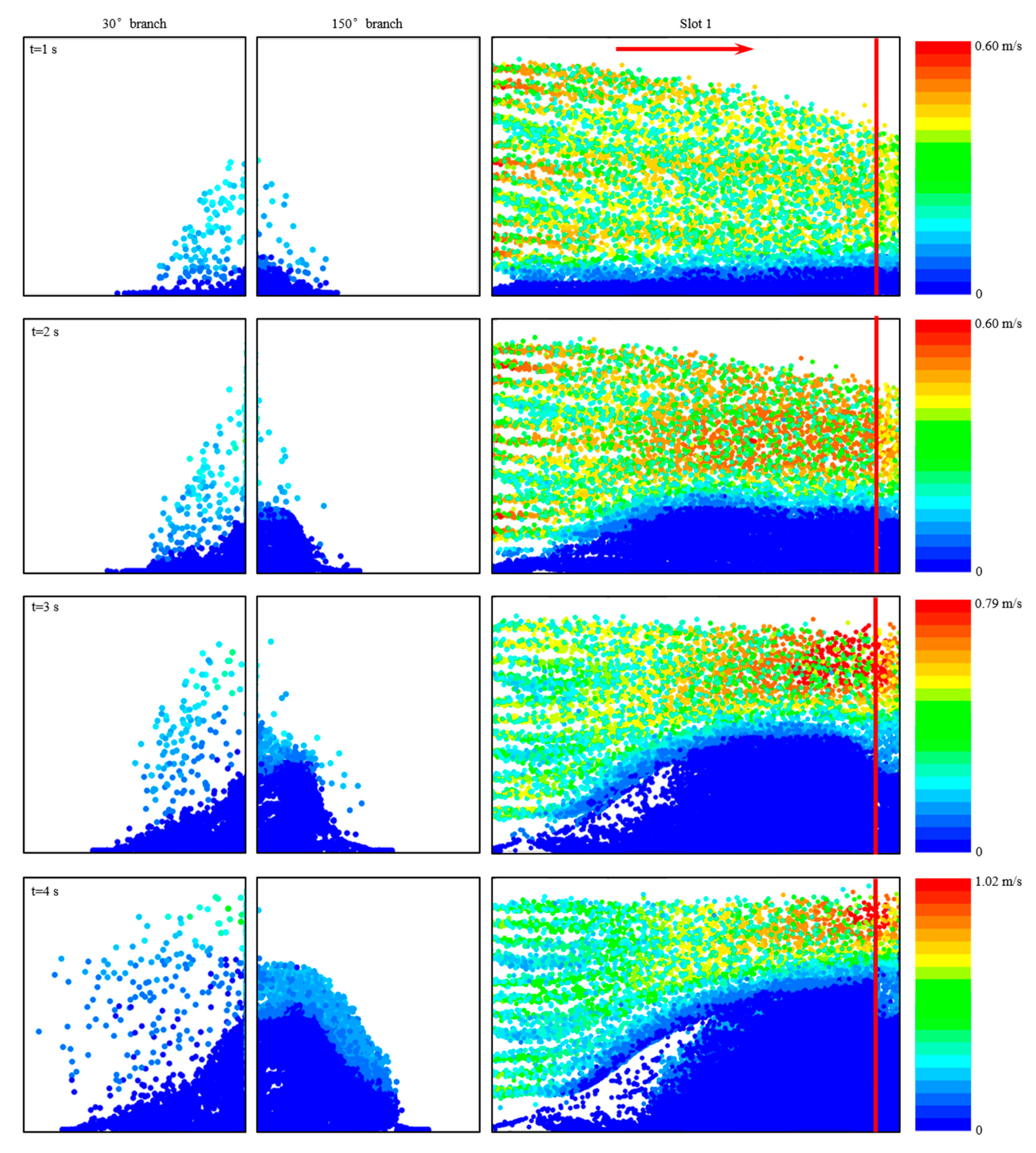
4.3.1. Model Validation

In this section, the model is validated by comparing the simulation results with the experimental results. Cases 1, 4 (with the 90°-orthogonal branch), and 12 (with 45–135°-branches) were simulated using this model. The normalized dune height, taken as the ratio of the dune height to the slot height, was adopted as the verification criterion. Figure 10 and Figure 11 presents the simulation results in cases 1 and 4, respectively. The normalized dune heights in slots 1, 2, 3, and the 90°-branch were observed. In each slot, the heights at one-third and two-thirds of the slot length were chosen for comparison. Experimental results in cases 1 and 4 are presented in Figure 3. For case 1, the dune geometries at 30%, 60%, and 90% of the total sand pumped are identified in Figure 10a and presented in Figure 10b. It was indicated that in slots 2, 3, and the 90°-branch, simulation results agree well with the experimental results. In slot 1, especially at the position closer to the inlet, it can be found that the simulation results slightly deviate from the experimental results, with a maximum deviation of about 34%. This is probably due to the turbulent effect near the inlet, with the dune eroded. For case 4, the dune geometries at the same three pumping stages are identified in Figure 11a and presented in Figure 11b. Similarly, there is a good agreement between the simulation and experimental results in slots 2 and 3. The turbulent effects near the inlet may cause a deviation. Due to the pressure outlet, some particles may flow out of the computation domain, which causes a reduction of the normalized dune height in the 90°-branch. Despite the deviation, it is considered that the numerical simulation model with a 90°-branch used in this study is reliable with the allowable engineering error.
Afterward, the model with 45–135°-branches is validated using case 12. The normalized dune heights in the two branches were observed. In each slot, the heights at the normalized dune length (i.e., the ratio of the dune length to the slot length) of 0.1, 0.3, 0.5, 0.7, and 0.9 were chosen for comparison. Experimental results in case 12 are presented in Figure 8. Also, the dune geometries at 30%, 60%, and 90% of the total sand pumped are identified and presented in Figure 12. It was demonstrated that the simulated results are close to the experimental values with a maximum deviation of less than 25%. Overall, the errors produced from the model with two branches is acceptable in engineering and can be applied for further study.

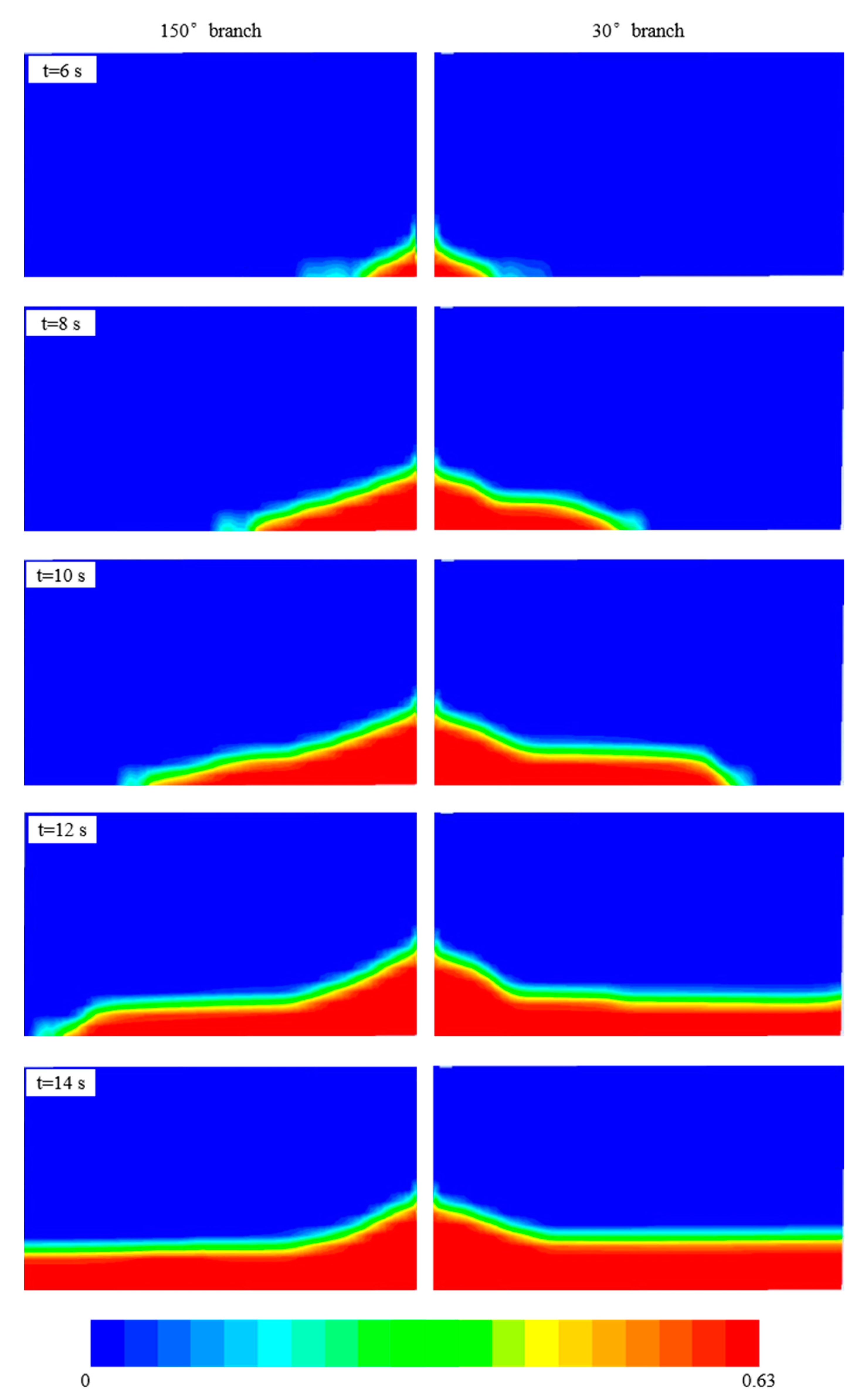
4.3.2. Dune Development in Branches at Different Locations

With the branch at different locations, proppant transport in the complex fracture system was simulated. For all numerical simulations, the same amount of sand was injected. First of all, the numerical and experimental results were compared. From Figure 13, the numerical results matched well with the experimental results in the branch with a large angle (i.e., 135°-branch and 150°-branch). However, there is a discrepancy between the numerical and experimental results in the branch with a small angle (i.e., 45°-branch and 30°-branch). In the numerical model, the branch length is set to 0.5 m, and the branch height is set to 0.06 m. Although the model domain was scaled based on the geometry similarity criterion, the proppant diameter set in the simulation was the same as that in the field. As a result, the horizontal transport distance in the branch obtained in the numerical simulation was shorter than that in the experiment. More proppants injected would flow out of the branch through the outlet on the branch top before they settled on the bottom.
According to Figure 13, the placement area in the branch decreased with the increasing distance from the inlet, and the placement area in the branch with a larger angle tended to be larger than that with a smaller angle. When the branch was placed at the position 100 mm away from the inlet, the placement areas in the 90°-, 135°-, and 150°-branches were larger than those in the 30°- and 45°-branches, and there were few differences for the placement area among the 90°-, 135°-, and 150°-branches. When the branch was placed at the position 200 mm away from the inlet, the placement areas in the 90°-, 135°-, and 150°-branches were still larger than those in the 30°- and 45°-branches, but the gap between these two categories of branches narrowed. When the branch was placed at the position 400 mm away from the inlet, the placement areas among these branches were approximately the same.
When the branch was far from the inlet, most proppants injected tended to settle in the primary fracture before they transported to the intersection. Thus, the branches situated at the deep of a primary fracture may not be well propped by the sand. To solve the issue, more proppants should be injected to prop those branches. As a result, the corresponding sand amount may be considerable and the operation time would increase significantly.

4.3.3. Dune Development in Branches under a Low Pumping Rate

It was found from Figure 14 that when the branch was near the inlet, an orthogonal branch possessed the largest placement area. In a branch with a small angle, proppants tended to travel a long distance and settle along the branch length. Due to an open system used in this study, the proppants would transport out of the system, which caused some proppants not to settle in the branch. Figure 11 described the mechanism of proppant transport into the 30°- and 150°-branches.
Figure 11 indicates that a suspended layer and a rolling layer occurred on the dune top in slot 1. However, the thickness of the suspended layer was much thicker than that of the rolling layer. At t = 1 s, the velocity of proppants at the intersection was approximately 0.4 m/s. A few proppants from the suspended layer turned the corner at the intersection and entered the two branches. They quickly settled due to the decreased flow rate in the branch. Meanwhile, a small number of proppants from the rolling layer rolled into the two branches, and accumulated on the dune top.
As the dune height in slot 1 increased, the proppant velocity increased correspondingly. At t = 4 s, the highest proppant velocity magnitude increased to 1.02 m/s. Behaviors for the proppants to enter the two branches changed. Proppants from the suspended layer mainly transported into the 30°-branch. These proppants could be carried by the fluid to the fracture tip, and some which did not settle in the branch flew out of the system through the outlet. Additionally, some proppants in the rolling layer fell into the 30°-branch due to gravity. These proppants accumulated near the branch inlet. Proppants from the rolling layer mainly entered the 150°-branch. They rolled on the branch dune and contributed to the height increase. Due to a low particle velocity, these proppants cannot transport to the deep of the branch and would not flow out of the system.
Combining the numerical results with the experimental results, it was concluded that the pressure outlet in the apparatus and numerical model had an effect on the placement area in the branch with a small angle. Due to the size limit, the branch length used in laboratories cannot satisfy a long horizontal transport distance, causing proppants to flow out of the fracture system. One more simulation under a low pumping rate was conducted below, and the dune development in the two branches are presented in Figure 15. It was found that proppants started to enter the two branches at t = 6 s, before which proppants mainly settled in the primary fracture. At this time, the dune geometry and placement area were almost the same in the 30°- and 150°-branches. As more proppants were injected, the dune in the two branches gradually developed. Different from the results in Figure 14, the dune in the 30°-branch developed slightly faster than that in the 150°-branch, and the dune front in the 30°-branch reached the boundary earlier than that in the 150°-branch. This demonstrated that the placement area in the 30°-branch was actually larger than that in the 150°-branch. Under a low pumping rate, the proppants entering the 30°-branch settled quickly, and they would not flow out of the system.

5. Conclusions

This study focused on the proppant transport and distribution in the complex fracture system. Slot flow experiments were conducted and CFD simulations were carried out with DDPM. The effects of the pumping rate, sand ratio, sand size, and branch angle and location on the proppant transport were studied. Some main conclusions are presented below:
(1)
The flow rate in the primary fracture is partitioned when encountering an intersection. In the case of a 90°-branch, approximately half of the slurry enter the secondary fracture. In the case of two branches, more than 60% of the slurry turn the corner into the branches. As the number of branches that the primary slot encounters increases, the flow rate remaining in the primary slot will decrease correspondingly. It is also found that the flow rate in the branch with a smaller angle is higher than the other with a larger angle.
(2)
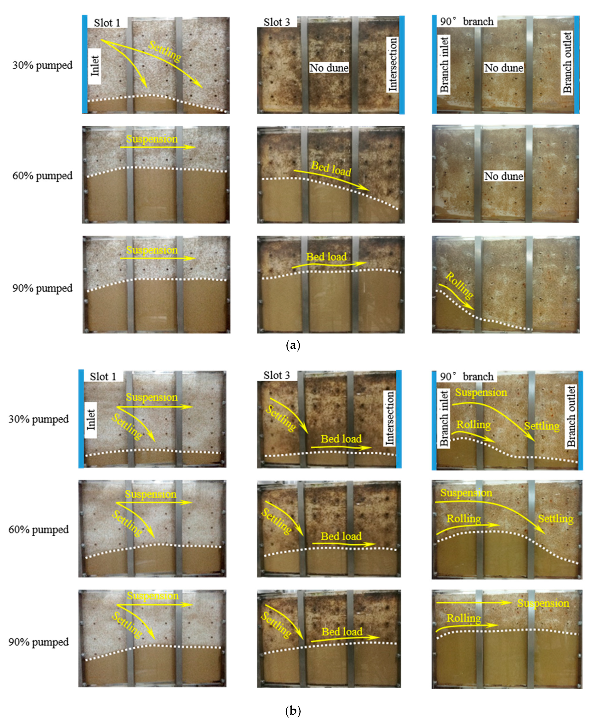
Two categories of dune development patterns in the complex fracture system are observed in the experiments. One pattern is that the dune development in the subsequent slot is dependent on the development degree of the dune in the precedent fracture; the other pattern is that the dunes in the primary fracture and branch can develop simultaneously.
(3)
Under a low pumping rate, the dune in the branch starts to develop only if the dune in the primary fracture has fully developed. Under a high pumping rate, a large of proppants can transport to the branch and the deep of a primary fracture. However, the proportion of sand which transport into the branch is lower than that in the case with a low pumping rate.
(4)
Sand ratio has few effects on the proppant distribution in the before-intersection fraction of a primary fracture, but has a significant impact on the proppant distribution in the branch and the after-intersection fraction of a primary fracture. A high sand ratio can result in a low proportion of proppant transporting into the branch, despite a high placement area in the branch due to the large sand amount injected. A low sand ratio leads to poor placement in the branch, but a higher proportion of proppant transporting into the branch can be obtained.
(5)
The branch and the deep of the primary fracture can be uniformly covered by fine proppants. However, a higher proportion of proppant transporting into the branch may be obtained in the final stage of the injection using the coarse proppants.
(6)
Uneven distribution of proppants can occur in the secondary fracture. Proppants tend to settle along the fracture length in the branch with a small angle, but tend to accumulate along the height in the branch with a large angle. The branch near the fracture inlet can obtain more proppants. Due to the size limit, a long horizontal transport distance cannot be realized in the branch with a small angle, and they will travel out of the system. As a result, a phenomenon that the placement area in the large-angle branch is larger than that in the small-angle branch. Decreasing the experimental pumping rate or extending the branch length is an effective method to prevent the proppants from flowing out of the system.
In future work, the presented results will be extended to the field scale. For the experimental results, the placement areas in the slot should be used to predict those in the real fractures, especially in the natural fractures. For the numerical simulation, the model can be improved to consider the effects of tortuosity and leak-off. Also, a large-scale model with an acceptable cost and satisfying engineering accuracy is also needed to extrapolate the results.

Author Contributions

Conceptualization, S.Z.; Formal analysis, Z.Z.; Investigation, Z.Z. and W.Z.; Methodology, Z.Z., X.M. and T.G.; Writing—original draft, Z.Z.; Writing—review & editing, Y.Z. All authors have read and agreed to the published version of the manuscript.

Funding

This research was supported by the National Natural Science Foundation of China (No. 51574255; No.51704305) and the National Major Science and Technology Projects of China (No. 2017ZX05049-006).

Acknowledgments

The authors would like to thank the anonymous reviewers for the valuable comments.

Conflicts of Interest

The authors declare no conflict of interest.

Appendix A

Figure A1. Design drawing of the slot system, (a) schematic of a single slot, (b) top view of the fracture system.
Energies 13 06290 g0a1

References

  1. Maxwell, S.C.; Urbancic, T.I.; Steinsberger, N.; Zinno, R. Microseismic imaging of hydraulic fracture complexity in the Barnett Shale. In Proceedings of the SPE Annual Technical Conference and Exhibition, San Antonio, TX, USA, 29 September–2 October 2002. [Google Scholar]
  2. Cipolla, C.L.; Warpinski, N.R.; Mayerhofer, M.J.; Lolon, E.P.; Vincent, M.C. The relationship between fracture complexity, reservoir properties, and fracture-treatment design. SPE Prod. Oper. 2010, 25, 438–452. [Google Scholar] [CrossRef]
  3. Zou, Y.S.; Ma, X.F.; Zhou, T.; Li, N.; Chen, M.; Li, S.H.; Zhang, Y.N.; Li, H. Hydraulic fracture growth in a layered formation based on fracturing experiments and discrete element modeling. Rock Mech. Rock Eng. 2017, 50, 2381–2395. [Google Scholar]
  4. Sahai, R.; Moghanloo, R.G. Proppant transport in complex fracture networks–A review. J. Petrol. Sci. Eng. 2019, 182, Article 106199. [Google Scholar] [CrossRef]
  5. Mckenna, J.P. Where did the proppant go? In Proceedings of the Unconventional Resources Technology Conference, Denver, CO, USA, 25–27 August 2014. [Google Scholar]
  6. Tan, P.; Jin, Y.; Hou, B.; Zheng, X.; Guo, X.; Gao, J. Experiments and analysis on hydraulic sand fracturing by an improved true tri-axial cell. J. Petrol. Sci. Eng. 2017, 158, 766–774. [Google Scholar] [CrossRef]
  7. King, G.E. Thirty years of gas shale fracturing: What have we learned? In Proceedings of the SPE Annual Technical Conference and Exhibition, Florence, Italy, 19–22 September 2010. [Google Scholar]
  8. Britt, L.K.; Smith, M.B.; Haddad, Z.; Lawrence, P.; Chipperfield, S.; Hellman, T. Water-fracs: We do need proppant after all. In Proceedings of the SPE Annual Technical Conference and Exhibition, San Antonio, TX, USA, 24–27 September 2006. [Google Scholar]
  9. Sahai, R. Laboratory Evaluation of Proppant Transport in Complex Fracture Systems; Colorado School of Mines: Golden, CO, USA, 2012. [Google Scholar]
  10. Kern, L.R.; Perkins, T.K.; Wyant, R.E. The mechanics of sand movement in fracturing. J. Petrol. Technol. 1959, 11, 55–57. [Google Scholar] [CrossRef]
  11. Medlin, W.L.; Sexton, J.H.; Zumwalt, G.L. Sand transport experiments in thin fluids. In Proceedings of the SPE Annual Technical Conference and Exhibition, Las Vegas, NV, USA, 22–26 September 1985. [Google Scholar]
  12. Liu, Y.; Sharma, M.M. Effect of fracture width and fluid rheology on proppant settling and retardation: An experimental study. In Proceedings of the SPE Annual Technical Conference and Exhibition, Dallas, TX, USA, 9–12 October 2005. [Google Scholar]
  13. Brannon, H.D.; Wood, W.D.; Wheeler, R.S. Large scale laboratory investigation of the effects of proppant and fracturing fluid properties on transport. In Proceedings of the SPE International Symposium and Exhibition on Formation Damage Control, Lafayette, LA, USA, 15–17 February 2006. [Google Scholar]
  14. Fernández, M.E.; Sánchez, M.; Pugnaloni, L.A. Proppant transport in a scaled vertical planar fracture: Vorticity and dune placement. J. Petrol. Sci. Eng. 2019, 173, 1382–1389. [Google Scholar] [CrossRef]
  15. Raimbay, A.; Babadagli, T.; Kuru, E.; Develi, K. Quantitative and visual analysis of proppant transport in rough fractures. J. Nat. Gas Sci. Eng. 2017, 33, 1291–1307. [Google Scholar] [CrossRef]
  16. Patankar, N.A.; Joseph, D.D.; Wang, J.; Barree, R.D.; Conway, M.; Asadi, M. Power law correlations for sediment transport in pressure driven channel flows. Int. J. Multiphas. Flow 2002, 28, 1269–1292. [Google Scholar] [CrossRef] [Green Version]
  17. Wang, J.; Joseph, D.D.; Patankar, N.A.; Conway, M.; Barree, R.D. Bi-power law correlations for sediment transport in pressure driven channel flows. Int. J. Multiphas. Flow 2003, 29, 475–494. [Google Scholar] [CrossRef]
  18. Sahai, R.; Miskimins, J.L.; Olson, K.E. Laboratory results of proppant transport in complex fracture systems. In Proceedings of the SPE Hydraulic Fracturing Technology Conference, The Woodlands, TX, USA, 4–6 February 2014. [Google Scholar]
  19. Tong, S.; Mohanty, K.K. Proppant transport study in fractures with intersections. Fuel 2016, 181, 463–477. [Google Scholar] [CrossRef]
  20. Alotaibi, M.A.; Miskimins, J.L. Slickwater proppant transport in hydraulic fractures - new experimental findings and scalable correlation. SPE Prod. Oper. 2018, 33, 164–178. [Google Scholar] [CrossRef]
  21. Li, N.; Li, J.; Zhao, L.; Luo, Z.; Liu, P.; Guo, Y. Laboratory testing on proppant transport in complex-fracture systems. SPE Prod. Oper. 2017, 32, 382–391. [Google Scholar] [CrossRef]
  22. Pan, L.; Zhang, Y.; Cheng, L.; Lu, Z.; Kang, Y.; He, P.; Dong, B. Migration and distribution of complex fracture proppant in shale reservoir volume fracturing (In Chinese). Natur. Gas Ind. 2018, 38, 61–70. [Google Scholar]
  23. Ma, W.; Perng, J.; Tomac, I. Experimental investigation of proppant flow and transport dynamics through fracture intersections. arXiv 2020, arXiv:2009.09986. [Google Scholar]
  24. Zhang, G.; Li, M.; Gutierrez, M. Simulation of the transport and placement of multi-sized proppant in hydraulic fractures using a coupled CFD-DEM approach. Adv. Powder Technol. 2017, 28, 1704–1718. [Google Scholar] [CrossRef]
  25. Zhang, G.; Gutierrez, M.; Li, M. A coupled CFD-DEM approach to model particle-fluid mixture transport between two parallel plates to improve understanding of proppant micromechanics in hydraulic fractures. Powder Technol. 2017, 308, 235–248. [Google Scholar] [CrossRef]
  26. Baldini, M.; Carlevaro, C.M.; Pugnaloni, L.A.; Sánchez, M. Numerical simulation of proppant transport in a planar fracture: A study of perforation placement and injection strategy. Int. J. Multiphas. Flow 2018, 109, 207–218. [Google Scholar] [CrossRef]
  27. Chen, X.; Wang, J. A comparison of two-fluid model, dense discrete particle model and CFD-DEM method for modeling impinging gas–solid flows. Powder Technol. 2014, 254, 94–102. [Google Scholar] [CrossRef]
  28. Zeng, J.; Li, H.; Zhang, D. Numerical simulation of proppant transport in hydraulic fracture with the upscaling CFD-DEM method. J. Nat. Gas Sci. Eng. 2016, 33, 264–277. [Google Scholar] [CrossRef]
  29. Hu, X.; Wu, K.; Li, G.; Tang, J.; Shen, Z. Effect of proppant addition schedule on the proppant distribution in a straight fracture for slickwater treatment. J. Petrol. Sci. Eng. 2018, 167, 110–119. [Google Scholar] [CrossRef]
  30. Mao, S.; Shang, Z.; Chun, S.; Li, J.; Wu, K. An efficient three-dimensional multiphase particle-in-cell model for proppant transport in the field scale. In Proceedings of the Unconventional Resources Technology Conference, Denver, CO, USA, 22–24 July 2019. [Google Scholar]
  31. Siddhamshetty, P.; Mao, S.; Wu, K.; Kwon, J.S. Multi-size proppant pumping schedule of hydraulic fracturing: Application to a MP-PIC model of unconventional reservoir for enhanced gas production. Processes 2020, 8, 570. [Google Scholar] [CrossRef]
  32. Zeng, J.; Li, H.; Zhang, D. Numerical simulation of proppant transport in propagating fractures with the multi-phase particle-in-cell method. Fuel 2019, 245, 316–335. [Google Scholar] [CrossRef]
  33. McClure, M. Bed load proppant transport during slickwater hydraulic fracturing: Insights from comparisons between published laboratory data and correlations for sediment and pipeline slurry transport. J. Petrol. Sci. Eng. 2018, 161, 599–610. [Google Scholar] [CrossRef] [Green Version]
  34. Zou, Y.S.; Zhang, S.C.; Ma, X.F.; Zhou, T.; Zeng, B. Numerical investigation of hydraulic fracture network propagation in naturally fractured shale formations. J. Struct. Geol. 2016, 84, 1–13. [Google Scholar] [CrossRef]
  35. Miller, M.C.; McCave, I.N.; Komar, P.D. Threshold of sediment motion under unidirectional currents. Sedimentology 1997, 24, 507–527. [Google Scholar] [CrossRef]
  36. Ogawa, S.; Umemura, A.; Oshima, N. On the equation of fully fluidized granular materials. J. Appl. Math. Phys. 1980, 31, 483–484. [Google Scholar] [CrossRef]
  37. Lun, C.K.; Savage, S.B.; Jeffrey, D.J.; Chepurniy, N. Kinetic theories for granular flow: Inelastic particles in Couette flow and slightly inelastic particles in a general flowfield. J. Fluid Mech. 1984, 140, 223–256. [Google Scholar] [CrossRef]
  38. Ding, J.; Gidaspow, D. A bubbling fluidization model using kinetic theory of granular flow. AIChE J. 1990, 36, 523–538. [Google Scholar] [CrossRef]
  39. Johnson, P.C.; Jackson, R. Frictional–collisional constitutive relations for granular materials, with application to plane shearing. J. Fluid Mech. 1987, 176, 67–93. [Google Scholar] [CrossRef]
  40. Cloete, S.; Johansen, S.T.; Amini, S. Performance evaluation of a complete Lagrangian KTGF approach for dilute granular flow modeling. Powder Technol. 2012, 226, 43–52. [Google Scholar] [CrossRef] [Green Version]
  41. Gidaspow, D. Multiphase Flow and Fluidization: Continuum and Kinetic Theory Descriptions; Academic Press: Cambridge, MA, USA, 1994. [Google Scholar]
  42. Ma, D.; Ahmadi, G. A thermodynamical formulation for dispersed multiphase turbulent flows. Int. J. Multiph. Flow 1990, 16, 323–351. [Google Scholar] [CrossRef]
  43. Shih, T.; Liou, W.W.; Shabbir, A.; Yang, Z.; Zhu, J. A new k-ε eddy viscosity model for high Reynolds number turbulent flows. Comput. Fluids 1995, 24, 227–238. [Google Scholar] [CrossRef]
Figure 1. Experimental apparatus, (a) photogragh of the real setup, (b) schematic of the experimental apparatus (to scale), (1) blender, (2) progressive cavity pump, (3) inlet, (4) outlets, (5) primary fracture, (6) secondary fractures, (7) magnetic flow meter, (8) valve, (9) sedimentation pool.
Energies 13 06290 g001
Figure 2. Schematic of the placement area and its increment in the slot.
Energies 13 06290 g002
Figure 3. Pattern of dune development in the branch, (a) the branch dune development is dependent on the dune in the primary fracture for case 1, (b) the branch dune development is independent on the dune in the primary fracture for case 4.
Energies 13 06290 g003
Figure 4. Evolvement of the dunes under different pumping rates, (a) case 1 under a pumping rate of 5.40 m3/h, (b) case 4 under a pumping rate of 12.60 m3/h.
Energies 13 06290 g004aEnergies 13 06290 g004b
Figure 5. Evolvement of the dunes under different sand ratios, (a) case 5 under a sand ratio of 4%, (b) case 6 under a sand ratio of 8%.
Energies 13 06290 g005
Figure 6. Evolvement of the dunes under different sand sizes, (a) case 7 under 16/20 proppants, (b) case 10 under 70/140 proppants.
Energies 13 06290 g006
Figure 7. Evolvement of dunes in a slot system with 30–150°-branches, (a) dune geometries in slot 1, slot 3 and branches when 30%, 60%, or 90% of sand were pumped, (b) placement areas in the primary and secondary slots, (c) distribution of sand injected in the primary and secondary slots.
Energies 13 06290 g007
Figure 8. Evolvement of dunes in a slot system with 45–135°-branches, (a) dune geometries in slot 1, slot 3 and branches when 30%, 60%, or 90% of sand were pumped, (b) placement areas in the primary and secondary slots, (c) distribution of sand injected in the primary and secondary slots.
Energies 13 06290 g008
Figure 9. Sketch of the computational geometries with branches at different locations, (a) 30–150°-branches, (b) 45–135°-branches, (c) 90°-branch.
Energies 13 06290 g009
Figure 10. Simulation and experimental results of normalized dune height for case 1, (a) Dune geometries in different pumping stages, (b) comparisons between simulation and experimental results.
Energies 13 06290 g010
Figure 11. Simulation and experimental results of normalized dune height for case 4, (a) Dune geometries in different pumping stages, (b) comparisons between simulation and experimental results.
Energies 13 06290 g011
Figure 12. Simulation and experimental results of normalized dune height for case 12.
Energies 13 06290 g012
Figure 13. Numerical results of dune development in the Branch at Different Locations.
Energies 13 06290 g013
Figure 14. Mechanism of proppant transport into the 30°- and 150°-branches.
Energies 13 06290 g014
Figure 15. Dune development in 30°- and 150°-branches under a low pumping rate.
Energies 13 06290 g015
Table 1. Values of experimental parameters and dimensionless quantities.
ParameterSlot SystemUnitFieldUnit
Fracture height H0.6m20m
Half-length of the primary fracture L5.0m167m
Width of the primary fracture w0.005m0.005m
Fluid density ρf1000kg/m31000kg/m3
Proppant density ρs3350kg/m33350kg/m3
Fluid viscosity μf0.001Pa·s0.001Pa·s
Proppant diameter ds0.0001–0.001m0.0001–0.001m
Darcy friction factor fD0.04 [33]-0.04 [33]-
Fluid Reynolds number Ref5000–11,667-5000–11,667-
Particle Reynolds number Rep100–980-100–980-
Shields number S0.065–1.825-0.065–1.825-
Mean velocity in the fracture vi0.5–1.2m/s0.5–1.2m/s
Pumping rate Q5.4–12.6m3/h360–840m3/h
Table 2. Experimental scheme of proppant transport in the complex fracture system.
CaseBranch Angle (°)Pumping Rate Q (m3/h)Sand Ratio (%)Proppant SizeProppant Amount (kg)
190 (a single branch)5.46.020/4042.0
290 (a single branch)7.86.020/4042.0
390 (a single branch)10.26.020/4042.0
490 (a single branch)12.66.020/4042.0
590 (a single branch)10.24.020/4028.0
690 (a single branch)10.28.020/4056.0
790 (a single branch)10.26.016/2042.0
890 (a single branch)10.26.030/5042.0
990 (a single branch)10.26.040/7042.0
1090 (a single branch)10.26.070/14042.0
1130/150 (two branches)12.66.020/4042.0
1245/135 (two branches)12.66.020/4042.0
Table 3. Monitoring results of the flow rate partition at the intersection.
CaseInflow Rate Qi (m3/h)Outflow Rate in the Branch Qb (m3/h)Outflow Rate in the Primary Slot Qp (m3/h)Qb/Qi
15.402.74 (90°-branch)2.660.507
27.803.91 (90°-branch)3.830.501
310.205.17 (90°-branch)5.010.507
412.606.64 (90°-branch)5.910.527
510.204.68 (90°-branch)5.570.459
610.204.98 (90°-branch)5.160.488
710.204.72 (90°-branch)5.410.463
810.205.29 (90°-branch)4.910.519
910.205.70 (90°-branch)4.440.559
1010.205.86 (90°-branch)4.340.575
1112.604.48 (30°-branch)
4.05 (150°-branch)
4.090.677
1212.604.23 (45°-branch)
3.70 (135°-branch)
4.570.629
Table 4. Values of parameters in CFD simulations.
ParameterUnitValue
Inlet fluid velocitym/s0.6
Inlet proppant velocitym/s0.6
Total proppant mass ratekg/s0.018
Proppant diameterm0.00064 (20/40 ceramic)
Fluid densitykg/m3998.2
Proppant densitykg/m33350
Angle of internal friction°30
Friction pressurePaBased KTGF
Friction modulusPaderived
Friction packing limit-0.61
Elasticity ModulusPaderived
Packing limit-0.63
Transition factor-0.75
Publisher’s Note: MDPI stays neutral with regard to jurisdictional claims in published maps and institutional affiliations.

