Study on Operating Strategy of Electric–Gas Combined System Considering the Improvement of Dispatchability

Abstract

The uncertainty of distributed energy (DG) and load in the electric–gas combined system (EGCS) requires EGCS to have higher dispatching capacity. A novel strategy is introduced in this paper to operate EGCS considering dispatchability evaluation indexes in order to improve the dispatchability of EGCS. Firstly, the paper describes the physical architecture of EGCS and its main devices. Based on the typical structure of EGCS, the main coupling modes between the two networks are analyzed and summarized, and a power flow model of deep coupling EGCS is established. Then, it proposes a unified quantitative modeling method of dispatchability, and qualitatively analyzes the dispatchability capability of different types of resources in the system through the definition, connotation, and multi-dimensional attributes of EGCS dispatchability. In order to characterize the strength of the overall dispatchability of EGCS, two evaluation indexes, upward/downward dispatchability margin, are proposed. The case study validates the applicability of the proposed dispatchability indexes through simulation. The uncertainties existing in various sources, namely networks and loads of EGCS, the output power of wind farms, and photovoltaic plants, are analyzed emphatically through actual data of a certain area. The EGCS economic dispatching model is established by considering the DG output prediction errors, introducing the expected penalty term of insufficient dispatchability into the objective function, and calculating the dispatchability margin through the simulation model to quantitatively analyze the dispatchability capability of the system.

1. Introduction

In recent years, with the increasingly obvious shortcomings of traditional energy and the rapid development of new energy technologies, Rifkin, an American economist, first put forward the concept of Energy internet in 2011 [1]. The concept focuses on replacing traditional energy with clean renewable energy so that we can reduce the proportion of traditional energy in industrial development and combines internet technology to realize interconnection, interoperability, and complementarity of current energy resources, which will maximize the efficiency of energy utilization. The energy network, which integrates new energy technology and information technology, has become the future direction of energy development [2,3].

With the construction of the Energy internet, the power system coordinated optimization mode of “source-network-load-storage” has become the core link of the development of Energy internet. This mode can be more widely applied to the whole energy industry and combine the technology and operation mode of Energy internet to form a coordinated and optimized operation mode of the whole energy system, as shown in Figure 1 [4].

Under this model, as a mature form of integrated energy network, electric–gas combined system (EGCS) has different ways and principles of coupling between the two networks, and their relationship is becoming closer. Recently, the study on EGCS is mainly manifested in power flow modeling, dispatching optimization, and security issues.

• How to model EGCS? Wei Zhang et al. established a mathematical model to evaluate the maximum power supply capability of EGCS from the perspective of the influence of the natural gas network on the power supply capability [5]. Under the premise of considering the gas pipeline constraints in the natural gas network, Cem Sahin et al. analyzed the degree of interaction between the electric–gas networks by simulation from the perspective of security, and the electric–gas joint risk assessment model is established [6]. Based on the economics, Yuan Hu et al. analyzed the multi-stage planning problem of EGCS through economic optimal model simulation [7,8].
• Calculate the power flow of EGCS. Because of the coupling between different energy forms in the EGCS, the traditional models and mechanisms for solving a pure power system or natural gas system are no longer suitable for solving the mixed power flow of EGCS. Seungwon An et al. firstly proposed that natural gas network be modeled by analogy to the grid, and then solved the gas network power flow by using the grid power flow calculation method [9]. Xiandong Xu et al. analyzed the power flow model in EGCS and studied the difference between mixed power flow and single power flow [10]; Sheng Chen et al. considered the calculation error problem caused by the uncertainty factors in the system, and solved the flow problem of EGCS by introducing the concept of probabilistic flow [11].
• There is a non-negligible uncertainty problem in EGCS [12,13,14,15]. From the perspective of energy output or utilization, the uncertainty can be distinguished as energy output side uncertainty and energy demand side uncertainty. The access of distributed energy (DG) will greatly increase the degree of uncertainty. Saeed Kamalinia et al. analyzed the influence of uncertainty degree of energy output or response on the economy or market mechanism of EGCS [16,17]. Zhinong Wei et al. provided a model description of the demand-side response of the system or the uncertainty of DG and formulates the operation strategy of EGCS by adding constraints involving uncertainty [18,19].
• Study the dispatching operation strategy of EGCS. Grid and the natural gas network are two kinds of networks with different energy sources. When they are coupled, the formulation of dispatching and operation strategy is different from that of a single network. Guoqing Li et al. analyzed the economy of wind power consumption under the condition of large proportion of wind power penetration and established a coordinated optimal dispatching model of integrated energy system considering power to gas (P2G) technology [20]. Chuan He et al. studied the joint planning problem of grid and natural gas network by ADMM technology [21]. Jiakun Fang et al. established an optimal dispatching model for integrated natural gas network and grid in order to improve consumption capacity of clean energy [22]. The above references respectively establish power flow or dispatching model for a single device unit or coupling device unit in EGCS, and formulate corresponding optimal operation strategies through some technical methods, but all of these references do not effectively evaluate the dispatchability of EGCS.

With the increasing capacity of wind, solar energy, and other DG connected to the power system, EGCS’s power generation and grid connection technology have become the hot issues concerned by the majority of power science and technology workers at present. Wind and solar energy have uncertainties such as stochastic fluctuation, intermittence, and conversion between different energy sources in the process of power generation, which makes the dispatching of EGCS more complicated, and even directly affects the dispatchability capacity and dispatchability requirement of the system during the dispatching time. Neglect of uncertainties in DG and load in the EGCS, and energy conversion losses, may lead to security and stability problems. Therefore, the establishment of a joint optimal dispatching model between grid and other DG has become a study hotspot. Jianxiao Wang et al. proposed a joint optimal dispatching scheme of energy and reserve based on microgrid combined cool, heat, and electric supply. Supported by the theory that heat supply has thermal inertia, the scheme considers that the reserve capacity of grid can be improved by the mutual conversion of different energy sources, and the conclusion is validated according to the actual data of Chicago Industrial Park in the United States [23]; Abigail D. Ondeck et al.’s study was based on the optimization of the current status of gas-heat power joint dispatching in residential quarters, and concluded that the optimization strategy has the characteristics of strong pertinence, multi-selectivity, and feedback interactivity [24]; Pedro Faria et al. simulated and analyzed the joint dispatching strategy considering demand response, and the simulation results show that this kind of dispatching strategy can greatly improve the efficiency of distributed energy utilization and reduce the operation cost of power system [25,26,27].

Therefore, the connectivity of DG and the grid has become the main trend of energy structure. However, EGCS has different coupling modes, and with the rapid development of the Energy internet, the access of a large number of DG and active loads increases the overall complexity of the system. The above references evaluate or optimize the uncertainties of the system due to the integration of new energy sources or active loads. However, there is no qualitative or quantitative analysis of the EGCS dispatchability with DG. There are currently no uniform indexes for EGCS dispatchability description. EGCS is more complicated than traditional grid or natural gas network, so the dispatching model of a single network needs to be improved to apply to the economic dispatching of EGCS. In addition, to accurately evaluate the dynamic characteristics of the system under the circumstance that consider the uncertainty of the system, it is necessary to quantify the dispatchability of energy and demand in the network, so as to formulate a more realistic dispatching operation strategy. For this purpose, this paper proposes an EGCS operation strategy study model considering dispatchability to correctly evaluate the dynamic characteristics of energy or load in the system, and makes qualitative analysis and quantitative calculation of dispatchability. Moreover, deterministic indexes to calculate dispatchability capability were proposed, so as to realize the optimum combination of dispatchable resources, which can improve the dispatchability of EGCS.

The major contributions of this paper are as follows.

• The power flow model of the EGCS is established in this paper.
• Through analyzing the factors influencing the uncertain performance capability of the system, two kinds of dispatchability evaluation indicators are proposed eventually, and their applicability is testified by simulation.
• To address the uncertainties in the source and load of EGCS, this paper analyzes the uncertainties of wind farms and photovoltaic plants output through actual data analysis in a certain area. Then, an economic dispatching model of EGCS considering DG output prediction errors is established, and the dispatchability under-expectation penalties is introduced into the objective function. On these foundations, this paper formulates the operation strategy of EGCS to improve the margin of the system.

The rest of this paper is organized as follows. In Section 2, an overview of EGCS is first provided. Then, an evaluation index of dispatchability on EGCS is presented in Section 3. This is followed by Section 4, in which the model of operation strategy for EGCS is presented. Eventually, Section 5 provides the case studies and the results from the case studies.

2. Overview of EGCS

2.1. Physical Structure and Devices of EGCS

The basic physical structure of EGCS is shown in Figure 2 [28]. According to the types of energy carried by the devices, all kinds of devices in the system can be divided into independent device unit and coupling device unit. An independent device unit, electric, heat, gas, and cool system maintains its own unique energy characteristics and there is no coupling transformation and complementary utilization between heterogeneous energy flows. Since the nature of cool load is similar to heat load, the following studies only consider heat load. The conversion between electric, heat, and gas can be realized by coupling device unit.

2.2. Coupling Relationship of EGCS

As a coupling device between power and natural gas, gas turbine uses natural gas as fuel, exists as load in natural gas network, and supplies the generated electricity to the grid as power on the grid side; in contrast to the role played by gas turbines in coupling, P2G can electrolyze water into hydrogen through electrolytic cells. The coupling method of EGCS is shown in Figure 3.

(1) Gas turbine

$$H_g=\omega +\epsilon P_G+\lambda P_G^2$$

(1)

where H_g denotes the calorific value of natural gas import into the gas turbine. P_G denotes the output power of the gas turbine. ω, ε and λ denote parameters for the heat consumption rate curve of the gas turbine.

(2) Electric drive compressor

In order to reduce gas loss, a pressurization station should be set up at a certain distance. When the compressor of pressurization station is driven by electric power, the relationship between input and output is shown in Equation (2).

$$P_{com}=\zeta H_{com}$$

(2)

where P_com is the power of the input compressor. H_com is the gas quantity of the output compressor. ζ = 7.457 × 10⁻⁶.

(3) Energy hub

The energy hub can enable the mutual conversion of heat-gas-power multiple energy forms. The specific structure of the energy hub is shown in Figure 4.

2.3. Power Flow Model of the Natural Gas Network

For gas pipelines, the gas flow F_mn through pipeline m-n under steady-state condition is calculated as follows:

$$F_{mn}=k_{mn}{s}_{mn}\sqrt{s_{mn}({\prod }_m^2-{\prod }_n^2)}$$

(3)

where k_mn is a constant and k_mn’s value is determined by inner diameter, length, efficiency, and compression factor of gas pipeline. s_mn reflects the direction of gas flow. П_m is the pressure of node m. П_n is the pressure of node n.

The flow balance equations of pressurization station are described as follows:

$$H_{com,k}=B_k{F}_{com,k}[{(\frac{{\prod }_m}{{\prod }_n})}^{Z_k}-1]$$

(4)

$${\tau }_{com,k}=\alpha +\beta H_{com,k}+\gamma H_{com,k}^2$$

(5)

where F_com,k is the flow through the pressurization station. τ_com,k is the flow consumed by the gas turbine. H_com,k is the power consumed by the compressor. α, β, and γ are the energy conversion efficiency constants. B_k and Z_k are constants.

The flow balance equation of node is expressed as follows:

$$F_m={\displaystyle \sum _{n\in m}{F}_{mn}+{\displaystyle \sum _{k\in m}\chi F_{com,k}+{\displaystyle \sum _{k\in m}{\tau }_{com,k}}}}$$

(6)

where F_m is the injection flow of the natural gas network node. ΣF_mn is the total flow of the pipe connected to the node. ΣχF_com,k is the total flow through the pressurization station, where χ = [1,−1], the inflow into the pressurization station is positive, and the outflow is negative. Στ_com,k is the self-depletion flow of the compressor driven by natural gas.

2.4. Network Structure of EGCS

The grid in EGCS operates independently of the natural gas network. The coupling method selected in this paper is the compressor of the pressurization station is driven by electric power, the gas turbine is driven by natural gas, and the energy hub is connected to realize the depth of “source-network-load” of IEEE30 and 14-bus natural gas system (NGS14). The network structure is shown in Figure 5.

3. Analysis of Dispatchability on EGCS

3.1. Overview of Dispatchability on EGCS

The dispatchability of the power system means that when there is rapid fluctuation on the energy side or load side of the power system, the system can still maintain continuous and reliable operation, which is an index to evaluate the balance of the power system [29]. Thus, the dispatchability of EGCS can be defined as the ability of the system to respond effectively to fluctuations in energy side (including thermal power, wind power, photovoltaic power, and natural gas power) or load side (including electric load, gas load, and heat load).

From the perspective of the system, the dispatchability of EGCS is a kind of ability to reflect whether the system can fully integrate and coordinate the dispatching resources within the system, effectively deal with various uncertain factors, flexibly adapt to various complex operating environments, and maintain the realization of the high-level operational objective.

3.2. Multidimensional Attributes of Dispatchability in EGCS

The dispatchability of EGCS not only needs to fully reflect the control and response of dispatching resources of different directions, different types, and different characteristics, but also needs to meet the dispatching and optimization requirements of the system in different cases. Figure 6 shows the multi-dimensional attribute feature representation of EGCS [30].

For EGCS, the essence of resolving the dispatchability problem is to meet different needs and coordinate the dispatching resources of different time, space, physical and value attributes by different means, so as to formulate the dispatch or operational strategies that meet specific time and space scales, are economical, practical, and physically achievable, and further meet the system requirements.

3.3. Evaluation Index of Dispatchability on EGCS

The dispatchability indexes of the traditional power system usually include parameters such as adjustable power range, output, or load regulation rate. For EGCS, the concept of dispatchability can be analogized, and the supply and demand of dispatchability of power side, network side, and load side can be quantitatively analyzed.

(1) Dispatchability analysis of conventional power

The conventional power included in the EGCS studied in this paper include thermal power units and gas units, which are the main dispatching supply resources in the system. The upward/downward dispatchability is respectively F_G+ and F_G−, as shown in Equations (7) and (8):

$$F_{\mathrm{G}+}=P_{\mathrm{Gmax}}-P_{\mathrm{G}},$$

(7)

$$F_{\mathrm{G}-}=P_{\mathrm{G}}-P_{\mathrm{Gmin}},$$

(8)

where P_G is the real-time output of the unit. P_Gmax and P_Gmin are, respectively, the maximum and minimum output of the unit.

The sum of Equations (7) and (8) can obtain the total amount of dispatching resources F_G that can be provided by conventional units, as shown in Equation (9):

$$F_{\mathrm{G}}=P_{\mathrm{G}\max }-P_{\mathrm{G}\min }.$$

(9)

(2) ispatchability analysis of distributed energy

Distributed energy such as wind and photovoltaic cannot be as stable and controllable as conventional power. Therefore, in the process of power balance, the output of the distributed energy is equivalent to the conventional power according to the given confidence capacity, while the remaining part is the un confidence capacity caused by the prediction error, which consumes the dispatchable resources. Therefore, the dispatching resources that are provided and consumed are as shown Equations (10) and (11):

$$F_{\mathrm{res},t}=P_{\mathrm{cl},t}$$

(10)

$$D_{\mathrm{res},t}=P_{\mathrm{res},t}-P_{\mathrm{cl},\mathrm{t}}$$

(11)

where F_res,t is the dispatchability that renewable energy can provide in tth period. P_cl,t is the confidence capacity. in tth period. D_res,t is the dispatchability of renewable energy consumption in tth period. P_res,t is the output power of renewable energy in tth period.

(3) Dispatchability analysis of controllable load

The controllable load can be regarded as a “conventional power” on the load side because of the load’s ability to be artificially adjusted. The dispatchability provided can be calculated according to Equation (9).

(4) Dispatchability analysis of uncontrollable load

The uncontrollable load is a resource that consumes dispatchability. Usually, the system will reserve a part of the backup capacity according to the historical maximum load when setting up the start-up mode, and the backup coefficient will be expressed as µ. The load’s demand for dispatching resources is shown in Equation (12):

$$D_{\mathrm{load}}=\mu P_{\mathrm{load},\max }+(P_{\mathrm{load},\max }-P_{\mathrm{load},\min })$$

(12)

where D_load is the dispatchability of uncontrollable load consumption. P_load,max and P_load,min are, respectively, peak and valley values of day-ahead load forecasting.

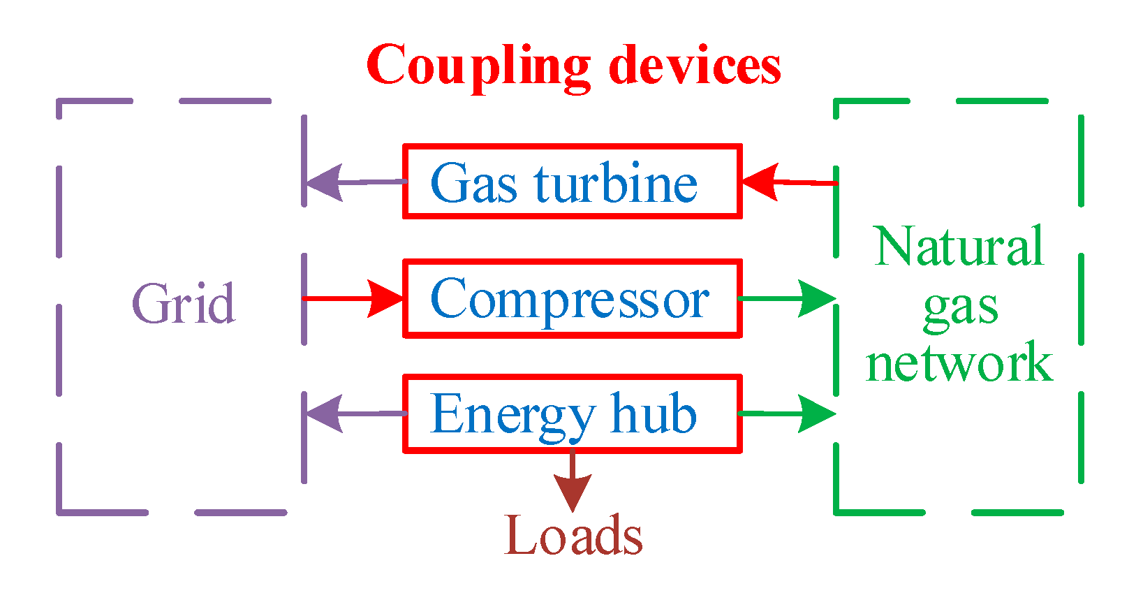
(5) Dispatchability analysis of network side energy conversion

There are different types of energy conversion on the network side of EGCS. Take P2G as an example. When the natural gas capacity in the network is insufficient and the electricity is surplus, the energy can be converted to natural gas through the energy conversion device. At this time, power can be regarded as the source side energy. The power’s dispatchability analysis is similar to the conventional power dispatchability analysis, there is a problem of energy conversion efficiency because the network side energy conversion is a conversion between different energy sources. Therefore, the dispatchability calculation of network side energy conversion in the link of P2G is shown in Equation (13).

$$F_{\mathrm{P}2\mathrm{G}}={\eta }_{\mathrm{P}2\mathrm{G}}{P}_{\mathrm{P}2\mathrm{G}}-C_{\mathrm{P}2\mathrm{G}}$$

(13)

where F_P2G is the dispatchability of P2G devices. η_P2G is the energy conversion efficiency of P2G devices. P_P2G is the electric power input to P2G devices. C_P2G is the natural gas power output by P2G devices.

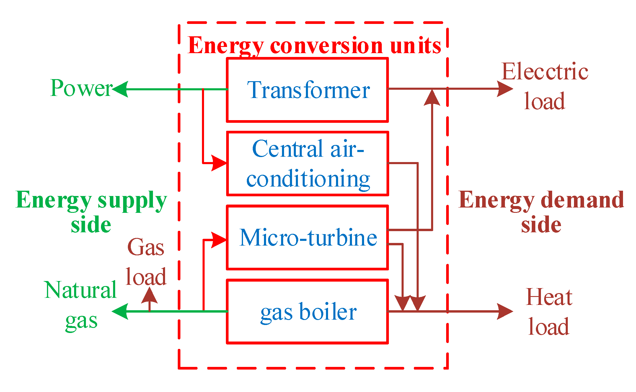
The controllable load and uncontrollable load mentioned in this paper include electric load, gas load, and heat load. Since the studied network is a grid and natural gas network, the heat load is equivalent to electric load and gas load.

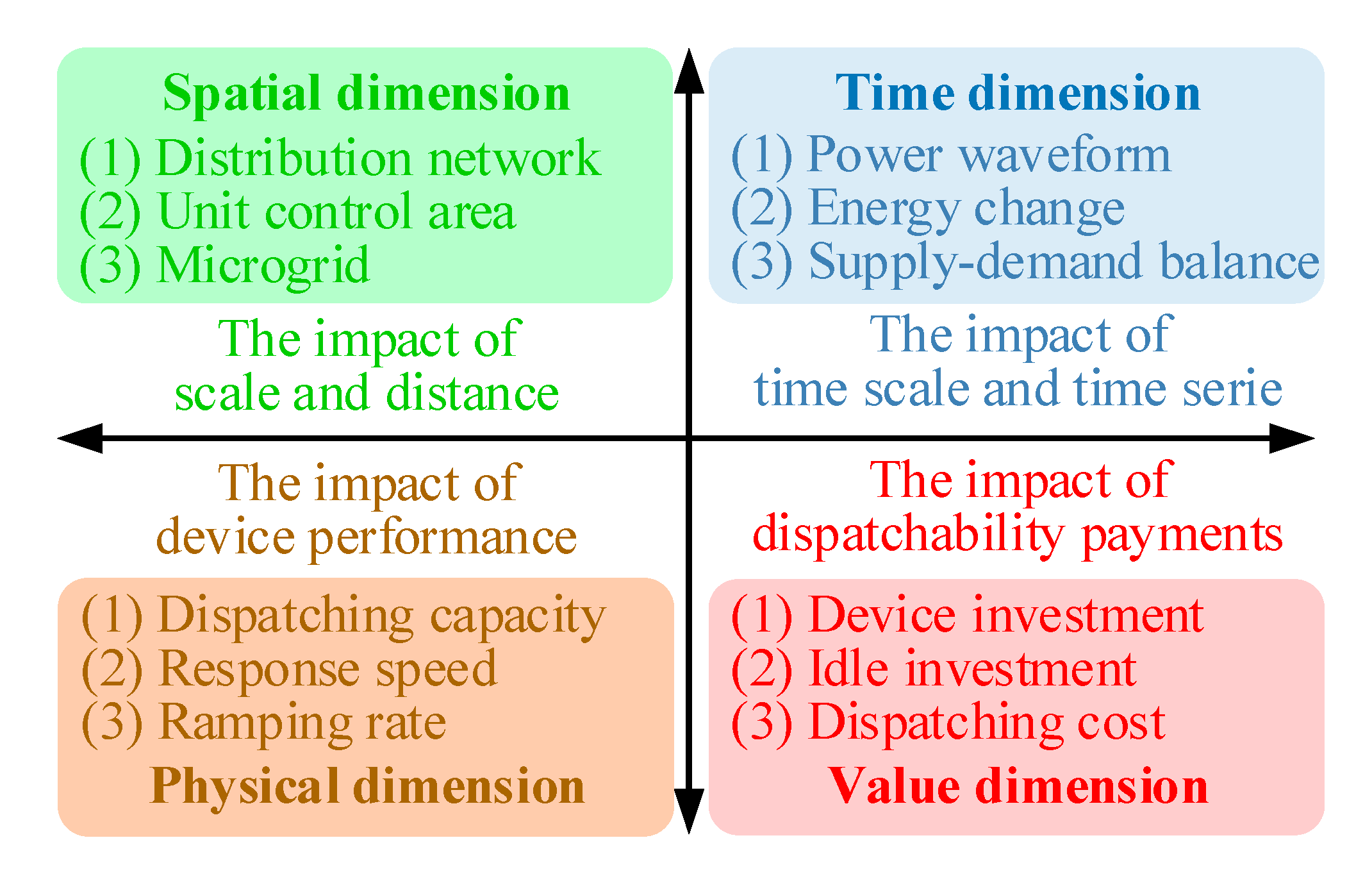
According to the multi-dimensional attributes of dispatchability and the quantitative analysis of dispatchability of different types of resources, various factors that need to be considered in establishing the EGCS dispatchability indexes can be obtained as shown in

Table 1. Factors to be considered in establishing EGCS dispatchability indexes.

Spatial Dimension	Time Dimension	Physical Dimension	Value Dimension
Electricity balance	Ramping rate of thermal power units	Available dispatching capacity of thermal power units	Operation cost of thermal power units
Flow balance
Conversion efficiency of power to gas	Power fluctuation of wind turbines	Available dispatching capacity of nature gas units	Operation cost of nature gas units
Conversion efficiency of gas to power
Conversion efficiency of power to heat	Power fluctuation of photovoltaic units
Conversion efficiency of gas to heat

.

As shown in Table 1, electricity balance and flow balance are the prerequisites for the secure and stable operation of the grid and natural gas network, and they must be met. Therefore, they are regarded as constraint conditions of dispatching model. The ramping rate and energy conversion efficiency of units are inherent characteristics of EGCS dispatchability, which cannot be changed after being put into operation. Therefore, they exist as general parameters in the calculation of dispatchability index or constraints. The value dimension parameters can be used as the objective function of the dispatching model to evaluate the dispatchability of the system from the economic point of view. Most importantly, due to the influence of natural factors and prediction errors, the output of wind turbines and photovoltaic units will be uncertain in time scale. At the same time, the available regulating capacity of conventional units will fluctuate with the switching state on time scale. These factors will directly affect the system’s upward and downward ability in the dispatching stage; that is, the factors have a great impact on the system’s dispatchability. Moreover, the natural gas network is an inertial system, while the grid is a real-time system. Therefore, this paper uses natural gas system to regulate the power system. Considering the capacity of coordinated dispatching of conventional thermal power units, gas generating units, distributed wind, and photovoltaic units in the 24-h operation phase of EGCS, the random variation of load is also considered. Four dispatchability evaluation indexes are proposed.

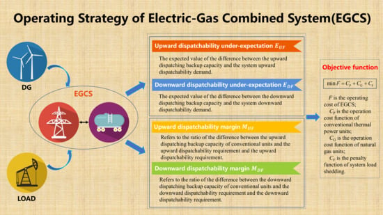
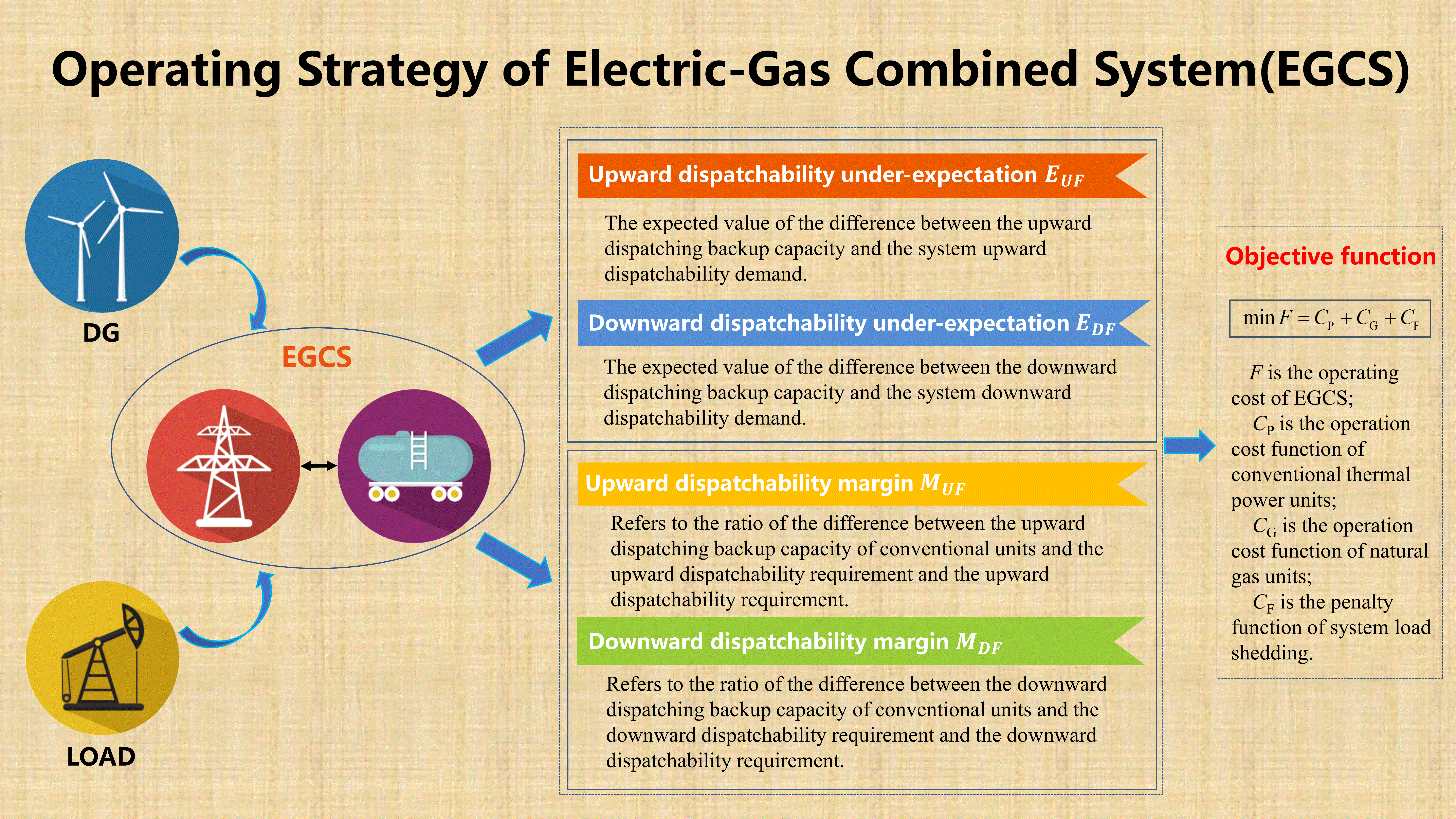
Index 1: Upward dispatchability under-expectation E_UF, is the expected value of the difference between the upward dispatching backup capacity and the system upward dispatchability demand in the system during the operation cycle. E_UF reflects the average value of the system’s failure to replenish resources when the consumption of dispatching resources increases, and the smaller the value, the better.

$$\{\begin{array}{l}\begin{array}{l}{E}_{\mathrm{UF},t}=\mathsf{\Delta }{R}_{\mathrm{UF},t}\mathrm{Pr}\left\{R_{\mathrm{UF},t}<P_{\mathrm{L},\mathrm{net},t+1}-P_{\mathrm{L},\mathrm{net},t}\right\}\\ \mathsf{\Delta }{R}_{\mathrm{UF},t}=P_{\mathrm{L},\mathrm{net},t+1}-P_{\mathrm{L},\mathrm{net},t}-R_{\mathrm{UF},t}\end{array}\hfill \\ R_{\mathrm{UF},t}=\min \left[{\displaystyle \sum _{i=1}^{N_{\mathrm{G}}}(P_{\mathrm{G}}^{i,t,\max }-P_{\mathrm{G}}^{i,t}),{\displaystyle \sum _{i=1}^{N_{\mathrm{G}}}{r}_{\mathrm{G},i}^{\mathrm{u}}\cdot \mathsf{\Delta }T}}\right]\hfill \end{array}$$

(14)

where R_UF,t is the upward dispatching backup capacity available for the system in tth period. P_L.net,t and P_L,net,t+1 are, respectively, the net load in tth and (t+1)th period. N_G is the total amount of natural gas units in the system. $P_{\mathrm{G}}^{i,t,\max }$ is the upper limit of the active power output of the ith conventional unit in tth period. $P_{\mathrm{G}}^{i,t}$ is the actual active output of the ith conventional unit in tth period. $r_{\mathrm{G},i}^{\mathrm{u}}$ is the upward ramping rate of the ith conventional unit. $\mathsf{\Delta }\mathrm{T}$ is the dispatching interval.

Index 2: Downward dispatchability under-expectation E_DF, is the expected value of the difference between the downward dispatching backup capacity and the system downward dispatchability demand in the system during the operation cycle. E_DF is reflected that when the resource that consumes dispatchability is reduced, the system cannot cut out the average value of supplied resources due to inertia and other problems, and the smaller the value, the better.

$$\{\begin{array}{l}\begin{array}{l}{E}_{\mathrm{DF},t}=\mathsf{\Delta }{R}_{\mathrm{DF},t}\mathrm{Pr}\left\{R_{\mathrm{DF},t}<P_{\mathrm{L},\mathrm{net},t}-P_{\mathrm{L},\mathrm{net},t+1}\right\}\\ \mathsf{\Delta }{R}_{\mathrm{DF},t}=P_{\mathrm{L},\mathrm{net},t}-P_{\mathrm{L},\mathrm{net},t+1}-R_{\mathrm{DF},t}\end{array}\hfill \\ R_{\mathrm{DF},t}=\min \left[{\displaystyle \sum _{i=1}^{N_{\mathrm{G}}}(P_{\mathrm{G}}^{i,t}-P_{\mathrm{G}}^{i,t,\min }),{\displaystyle \sum _{i=1}^{N_{\mathrm{G}}}{r}_{\mathrm{G},i}^{\mathrm{d}}\cdot \mathsf{\Delta }T}}\right]\hfill \end{array}$$

(15)

where R_DF,t is the downward dispatching backup capacity available for the system in tth period. $P_{\mathrm{G}}^{i,t,\min }$ is the lower limit of the active power output of the ith conventional unit in tth period. $r_{\mathrm{G},i}^{\mathrm{d}}$ is the downward ramping rate of the ith conventional unit.

Index 3: Upward dispatchability margin, M_UF, refers to the ratio of the difference between the upward dispatching backup capacity of conventional units and the upward dispatchability requirement of the system and the upward dispatchability requirement of the system during the operation period. M_UF reflects the adequacy level of dispatching resources that the system can provide when the increase in resources that consume dispatchability; the greater the value, the better.

$$\{\begin{array}{l}{M}_{\mathrm{UF},t}=\frac{R_{\mathrm{UF},t}-F_{\mathrm{UF},t}}{F_{\mathrm{UF},t}}\hfill \\ F_{\mathrm{UF},t}=P_{\mathrm{L},\mathrm{net},t+1}-P_{\mathrm{L},\mathrm{net},t}+{\displaystyle \sum _{w=1}^{N_{\mathrm{DG}}}(P_{\mathrm{DG},\mathrm{fc}}^{w,t}-P_{\mathrm{DG}}^{w,t})}\hfill \end{array}$$

(16)

where F_UF,t is the system’s upward dispatchability requirement in tth period. $P_{\mathrm{DG},\mathrm{fc}}^{w,t}$ is the predicted output power of the wth DG unit W in tth period. N_DG is the total amount of DG units. $P_{\mathrm{DG}}^{w,t}$ is the actual output power of the wth DG unit W in tth period.

Index 4: Downward dispatchability margin M_DF, refers to the ratio of the difference between the downward dispatching backup capacity of conventional units and the downward dispatchability requirement of the system and the downward dispatchability requirement of the system during the operation period. M_DF reflects the adequacy level of dispatching resources that the system can cut when the decrease in resources that consume dispatchability; the greater the value, the better.

$$\{\begin{array}{l}{M}_{\mathrm{DF},t}=\frac{R_{\mathrm{DF},t}-F_{\mathrm{DF},t}}{F_{\mathrm{DF},t}}\hfill \\ F_{\mathrm{DF},t}=P_{\mathrm{L},\mathrm{net},t}-P_{\mathrm{L},\mathrm{net},t+1}+{\displaystyle \sum _{w=1}^{N_{\mathrm{DG}}}(P_{\mathrm{DG}}^{w,t}-P_{\mathrm{DG},\mathrm{fc}}^{w,t})}\hfill \end{array}$$

(17)

where F_DF,t is the system’s downward dispatchability requirement in tth period.

The system operation must satisfy certain reliability. The above indexes 3 and 4 can indicate the reliability level of the system. However, due to the uncertain factors in the system, the current EGCS should try to achieve the optimal economy under the premise of ensuring the reliability of the system operation.

4. Model of Operation Strategy for EGCS

Compared with the traditional power system structure, EGCS is more complex, and the dimensions of EGCS dispatchability model for operation problems will be more abundant. Under the advancing of Energy internet negotiation, the operation strategy of EGCS through dispatchability evaluation aims to realize the optimal combination and dispatch of dispatching resources with the goal of multi-level dispatchability supply and demand matching of the system. Therefore, the joint optimization of EGCS is needed, which is essentially a mathematical programming problem involving equilibrium constraints, and optimizes the objective function of minimizing the total cost of the joint operation service supply by system operators.

4.1. Objective Function

The objective function that minimizes the operating cost of EGCS is expressed as follows:

$$\begin{array}{l}\min F=C_{\mathrm{P}}+C_{\mathrm{G}}+C_{\mathrm{F}}\\ \{\begin{array}{l}{C}_{\mathrm{P}}={\displaystyle \sum _{t=1}^T{\displaystyle \sum _{i=1}^{N_{\mathrm{P}}}\left[a_i+b_i{P}_{\mathrm{G}}^{i,t}+c_i{(P_{\mathrm{G}}^{i,t})}^2\right]}}\\ C_{\mathrm{G}}={\displaystyle \sum _{t=1}^T{\displaystyle \sum _{j=1}^{N_{\mathrm{G}}}{g}_j{P}_{\mathrm{gas}}^{j,t}}}\\ C_{\mathrm{F}}={\displaystyle \sum _{t=1}^T{c}_{\mathrm{F}}{E}_{\mathrm{F}}^t}\end{array}\end{array}$$

(18)

where F is the operating cost of EGCS. C_P is the operation cost function of conventional thermal power units. C_G is the operation cost function of natural gas units. C_F is the penalty function of system load shedding. T is the total amount of dispatching time periods in a dispatching cycle. N_P is the total amount of conventional thermal power units in the system. a_i, b_i, and c_i are the operating cost factors of the ith conventional thermal power unit. $P_{\mathrm{G}}^{i,t}$ is the output power of the ith conventional thermal power unit when the unit runs in tth period. N_G is the total amount of natural gas units in the system. g_j is the operating cost factor of the jth natural gas unit. $P_{\mathrm{gas}}^{\mathrm{j},t}$ is the output power of the jth natural gas unit when the unit runs in tth period. c_F is the cost factor of outage loss per unit load. $E_{\mathrm{F}}^t$ is the expected value of the system when the power is insufficient in tth period.

4.2. Constraints

(1) Power flow constraints:

$$\{\begin{array}{c}{P}_i=V_i{\displaystyle \sum _{j\in i}{V}_j}\left(G_{ij}\cos {\theta }_{ij}+B_{ij}\sin {\theta }_{ij}\right)\\ Q_i=V_i{\displaystyle \sum _{j\in i}{V}_j}\left(G_{ij}\sin {\theta }_{ij}-B_{ij}\cos {\theta }_{ij}\right)\end{array}$$

(19)

where P_i and Q_i are, respectively, the active and reactive power of node i. V_i is the voltage of node i. V_j is the voltage of node j. G_ij and B_ij are the line parameters between nodes i and j. θ_ij is the power factor of the line between nodes i and j.

(2) Power balance constraint:

$${\displaystyle \sum _{i=1}^{N_{\mathrm{P}}}{P}_{\mathrm{G}}^{i,t}+{\displaystyle \sum _{w=1}^{N_{\mathrm{DG}}}{P}_{DG}^{w,t}}}+{\displaystyle \sum _{v=1}^{N_{\mathrm{G}2\mathrm{P}}}{P}_{\mathrm{G}2\mathrm{P}}^{v,t}}-P_L^t+E_{\mathrm{F}}^t=0$$

(20)

where N_DG is the total amount of DG units. $P_{\mathrm{DG}}^{w,t}$ is the output power of the wth DG unit when the unit runs in tth period. N_G2P is the total amount of G2P units. $P_{\mathrm{G}2\mathrm{P}}^{v,t}$ is the output power of the vth G2P unit when the unit runs in tth period. $P_{\mathrm{L}}^t$ is the electric load. $E_{\mathrm{F}}^t$ is the expected value of the system when the power is insufficient in tth period.

(3) Upper and lower limit constraints of conventional unit output:

$$\{\begin{array}{l}{P}_{\mathrm{G}}^{i,\min }\le P_{\mathrm{G}}^i\le P_{\mathrm{G}}^{i,\max }\\ Q_{\mathrm{G}}^{i,\min }\le Q_{\mathrm{G}}^i\le Q_{\mathrm{G}}^{i,\max }\end{array}$$

(21)

where $P_{\mathrm{G}}^i$ and $Q_{\mathrm{G}}^i$ are, respectively, the active and reactive power output of the ith conventional unit. $P_{\mathrm{G}}^{i,\max }$ and $Q_{\mathrm{G}}^{i,\max }$ are respectively the upper limits of the active and reactive power output of the ith conventional unit. $P_{\mathrm{G}}^{i,\min }$ and $Q_{\mathrm{G}}^{i,\min }$ are, respectively, the lower limits of the active and reactive power output of the ith conventional unit.

(4) Constraint of DG output:

$$P_{\mathrm{DG}}^{w,\min }\le P_{\mathrm{DG}}^{w,t}+P_{\mathrm{DG}}^{w,t}\times e_{\mathrm{DG}}^{w,t}\le P_{\mathrm{DG}}^{w,\max }$$

(22)

where $P_{\mathrm{DG}}^{w,\min }$ and $P_{\mathrm{DG}}^{w,\max }$ are, respectively, the upper and lower limits of the active power output of the wth DG unit. $e_{\mathrm{DG}}^{w,t}$ is the prediction error of active power output of the wth DG unit in tth period.

(5) Ramping constraints:

$$\{\begin{array}{c}{P}_{\mathrm{G}}^{i,t+1}-P_{\mathrm{G}}^{i,t}\le u_{i,t}\cdot r_{\mathrm{G},i}^u\cdot \mathsf{\Delta }T+P_{\mathrm{G}}^{i,\max }(1-u_{i,t})\\ P_{\mathrm{G}}^{i,t}-P_{\mathrm{G}}^{i,t+1}\le u_{i,t+1}\cdot r_{\mathrm{G},i}^d\cdot \mathsf{\Delta }T+P_{\mathrm{G}}^{i,\max }(1-u_{i,t+1})\end{array}$$

(23)

where u_i,t is the switching state of the ith conventional unit in tth period, which is 0-1 vector, turn on is 1, turn off is 0. $r_{\mathrm{G},i}^u$ is the uphill ramping rate of the ith conventional unit. u_i,t+1 is the switching state of the ith conventional unit in (t+1)th period. $r_{\mathrm{G},i}^d$ is the downhill ramping rate of the ith conventional unit. $\mathsf{\Delta }T$ is the dispatching time.

(6) Constraint of node voltage:

$$U_i^{\min }\le U_{i,t}\le U_i^{\max }$$

(24)

where U_i,t is the voltage of node i in tth period. $U_i^{\max }$ and $U_i^{\min }$ are, respectively, the upper and lower limits of allowable voltage for node i.

(7) Constraint of line transmission power:

$$P_l^{\min }\le U_{i,t}{U}_{j,t}\left(G_{ij}\cos {\theta }_{ij}+B_{ij}\sin {\theta }_{ij}\right)-U_{i,t}^2{G}_{ij}\le P_l^{\max }$$

(25)

where $P_l^{\max }$ and $P_l^{\min }$ are, respectively, the upper and lower limits of active power allowable for transmission on line l.

(8) Grid reliability level constraint:

$$E_{\mathrm{F}}^t\le E_{\mathrm{F}}^{\max }$$

(26)

where $E_F^{\max }$ is the maximum allowable load shedding value of the system, indicating the reliability level of the system operation.

(9) Natural gas flow balance constraint:

$${\displaystyle \sum _{r=1}^{N_{\mathrm{G}}}{C}_{\mathrm{gas}}^{r,t}}+{\displaystyle \sum _{m=1}^{N_{\mathrm{P}2\mathrm{G}}}{C}_{\mathrm{P}2\mathrm{G}}^{m,t}}-{\displaystyle \sum _{n=1}^{N_{\mathrm{L}}}{C}_{\mathrm{line}}^{n,t}}-C_L^t=0$$

(27)

where $C_{\mathrm{gas}}^{r,t}$ is the gas flow output of the rth natural gas source in tth period. N_P2G is the total amount of P2G units. $C_{\mathrm{P}3\mathrm{G}}^{m,t}$ is the gas flow output of the mth P2G unit when the unit runs in tth period. N_L is the total amount of natural gas pipelines. $C_{\mathrm{line}}^{n,t}$ is the gas flow loss of the nth pipeline in tth period. $C_{\mathrm{L}}^t$ is the total natural gas load in tth period.

(10) Upper and lower limit constraint of nature gas unit output:

$$C_{\mathrm{gas}}^{r,\min }\le C_{\mathrm{gas}}^r\le C_{\mathrm{gas}}^{r,max}$$

(28)

where $C_{\mathrm{gas}}^r$ is the output of the rth natural gas unit. $C_{\mathrm{gas}}^{r,\min }$ and $C_{\mathrm{gas}}^{r,\max }$ are, respectively, the upper and lower limits of the output of the rth natural gas unit.

(11) Pipeline flow constraints:

$$\{\begin{array}{l}{C}_{\mathrm{line}}^n+C_{\mathrm{L},\mathrm{line}}^n\le C_{\mathrm{line}}^{n,\max }\hfill \\ C_{\mathrm{line}}^n=v_n{s}_n\sqrt{s_n\left({\mathsf{\Pi }}_{n_1}^2-{\mathsf{\Pi }}_{n_2}^2\right)}\hfill \\ s_n=\{\begin{array}{c}+1,{\mathsf{\Pi }}_{n_1}-{\mathsf{\Pi }}_{n_2}\ge 0\\ -1,{\mathsf{\Pi }}_{n_1}-{\mathsf{\Pi }}_{n_2}<0\end{array}\hfill \end{array}$$

(29)

where $C_{\mathrm{line}}^n$ is the flow of natural gas in pipe n. $C_{\mathrm{L},\mathrm{line}}^n$ is the total natural gas load supplied by pipeline n. $C_{\mathrm{line}}^{n,\max }$ is the maximum flow of natural gas in pipe n. v_n is constant. s_n reflects the direction of the pipeline flow. n₁ and n₂ are node numbers. П_n1 is the pressure of node n₁. П_n2 is the pressure of node n₂.

(12) Electric-gas coupling constraints:

$$\{\begin{array}{l}{H}_{\mathrm{g}}={\beta }_{\mathrm{g}}^1+{\beta }_{\mathrm{g}}^2{P}_{\mathrm{g}}+{\beta }_{\mathrm{g}}^3{P}_{\mathrm{g}}^2\hfill \\ C_{\mathrm{gas}}=\frac{H_{\mathrm{g}}}{GHV}\hfill \end{array}$$

(30)

where H_g is the input heat value of the gas turbine. P_g is the output power of the gas turbine. C_gas is the equivalent natural gas load of the node connected to the gas turbine in NGS14. GHV is a fixed high heat value. ${\beta }_{\mathrm{g}}^1$, ${\beta }_{\mathrm{g}}^2$, ${\beta }_{\mathrm{g}}^3$ are constants determined by the heat consumption rate curve of the gas turbine.

(13) Constraints of energy conversion efficiency

$$\{\begin{array}{l}{P}_{\mathrm{G}2\mathrm{P}}^{v,t}={\eta }_{\mathrm{G}2\mathrm{P}}^v{C}_{\mathrm{G}2\mathrm{P}}^{v,t}\\ C_{\mathrm{P}2\mathrm{G}}^{m,t}={\eta }_{\mathrm{P}2\mathrm{G}}^m{P}_{\mathrm{P}2\mathrm{G}}^{m,t}\\ H_{\mathrm{Heat}}^{s,t}={\eta }_{\mathrm{Heat}}^s{P}_{\mathrm{Heat}}^{s,t}\\ H_{\mathrm{Heat}}^{u,t}={\eta }_{\mathrm{Heat}}^u{C}_{\mathrm{Heat}}^{u,t}\end{array}$$

(31)

where $P_{\mathrm{G}2\mathrm{P}}^{v,t}$ is the output power of the vth G2P unit when the unit runs in tth period. $C_{\mathrm{G}2\mathrm{P}}^{v,t}$ is the gas flow input of the vth G2P unit when the unit runs in tth period. $C_{\mathrm{P}2\mathrm{G}}^{m,t}$ is the gas flow output of the mth P2G unit when the unit runs in tth period. $P_{\mathrm{P}2\mathrm{G}}^{m,t}$ is the input power of the mth P2G unit when the unit runs in tth period. $H_{\mathrm{Heat}}^{s,t}$ is the heat output of the sth power to heat unit when the unit runs in tth period. $P_{\mathrm{Heat}}^{s,t}$ is the power input of the sth power to heat unit when the unit runs in tth period. $H_{\mathrm{Heat}}^{k,t}$ is the heat output of the kth gas to heat unit when the unit runs in tth period. $C_{\mathrm{Heat}}^{k,t}$ is the gas flow input of the kth gas to heat unit when the unit runs in tth period. ${\eta }_{\mathrm{G}2\mathrm{P}}^v,$ ${\eta }_{\mathrm{P}2\mathrm{G}}^m$, ${\eta }_{\mathrm{Heat}}^s$, ${\eta }_{\mathrm{Heat}}^u$ are, respectively, the conversion efficiency of G2P device, P2G device, the power to heat device, and the gas to heat device.

Because the model is a nonconvex problem and cannot be solved by traditional optimization algorithms, heuristic algorithms are needed to solve the complex model, like particle swarm optimization (PSO) algorithm and genetic algorithm, etc. The particle in the PSO algorithm updates the position and velocity by tracking the local optimal solution and the global optimal solution, and keeps approaching to the optimal solution. PSO algorithm has faster convergence ability than the genetic algorithm in solving nonlinear functions. Simplified particle swarm optimization (SPSO) algorithm [31] is the improved algorithm of PSO algorithm. SPSO algorithm has no velocity term compared with PSO, so the evolution process of particles becomes simpler and easier to realize. Furthermore, SPSO algorithm can avoid trapping in local optimum and has faster convergence ability than PSO algorithm. Hence, the SPSO algorithm is appropriate to be used to solve the proposed model.

5. Case Study

5.1. Verify the Evaluation Index of Dispatchability on EGCS

In order to verify the rationality of dispatchability evaluation index, an economic dispatching model as shown in Equation (32) is established for the simple pure power system.

$$\begin{array}{l}\min F={\displaystyle \sum _{t=1}^T{\displaystyle \sum _{i=1}^{N_{\mathrm{P}}}\left[a_i+b_i{P}_{\mathrm{G}}^{i,t}+c_i{(P_{\mathrm{G}}^{i,t})}^2\right]}}+{\displaystyle \sum _{t=1}^T{c}_{\mathrm{F}}{E}_{\mathrm{F}}^t}\\ \mathrm{s}.\mathrm{t}.\{\begin{array}{l}{P}_{\mathrm{G}}^{i,t+1}-P_{\mathrm{G}}^{i,t}\le u_{i,t}\cdot r_{\mathrm{G},i}^u\cdot \mathsf{\Delta }T+P_{\mathrm{G}}^{i,\max }(1-u_{i,t})\\ {\displaystyle \sum _{i=1}^{N_{\mathrm{P}}}{P}_{\mathrm{G}}^{i,t}+E_{\mathrm{F}}^t}-P_L^t=0\\ P_{\mathrm{G}}^{i,\min }\le P_{\mathrm{G}}^i\le P_{\mathrm{G}}^{i,\max }\\ E_{\mathrm{F}}^t\le E_{\mathrm{F}}^{\max }\end{array}\end{array}$$

(32)

where a_i, b_i, and c_i are the operating cost factors of the ith conventional thermal power unit. c_F is the cost factor of outage loss per unit load. $E_{\mathrm{F}}^t$ is the expected value of the system when the power is insufficient in tth period. $E_{\mathrm{F}}^{\max }$ is the maximum allowable load shedding value of the system, indicating the reliability level of the system operation.

Based on the above model, the unit’s combination of the system at all time periods can be obtained, and the dispatchability capacity and dispatchability requirement for each period of the system can be obtained, thus the system dispatchability margin index M_UF and M_DF can be obtained. The dispatchability of the system is analyzed by using the three-machine three-node system as shown in Figure 7. The conventional units related parameters and load data are as shown in

Table 2. Parameters of the conventional units.

Unit	${\mathit{P}}_{\mathbf{G}}^{\mathit{i},\mathbf{max}}$/MW	${\mathit{P}}_{\mathbf{G}}^{\mathit{i},\mathbf{min}}$/MW	ai/($/MW2)	bi/($/MW)	ci/$	${\mathit{r}}_{\mathbf{G},\mathit{i}}^{\mathit{u}/\mathit{d}}$/(MW/min)
1	150	50	0.0020	30	500	2
2	100	20	0.0025	40	300	1.5
3	100	10	0.0050	20	100	1.5

and

Table 3. Load data.

Period/h	1	2	3	4
Load/MW	80	120	200	150

. $\mathsf{\Delta }T$ = 1 h, $c_F$ = $1500/M.

Firstly, without considering the reliability level of the system, the above economic dispatching model is solved under the three-machine system. The operating cost of the system is $28,076.9. The output and dispatching capacity allocation of each unit in the system are shown in

Table 4. Output of units and their dispatching capacity allocation.

Period/h	1	2	3	4
$P_{\mathrm{G}}^1$/MW	0	50	86.67	63.33
$P_{\mathrm{G}}^2$/MW	0	46.67	73.33	46.67
$P_{\mathrm{G}}^3$/MW	80	23.33	40	40
$R_{\mathrm{F}}^1$/MW	0	10	13.33	11.37
$R_{\mathrm{F}}^2$/MW	0	13.33	26.67	28.33
$R_{\mathrm{F}}^3$/MW	0	36.67	60	35
EF/MWh	1.6	0	0	0

. Based on this, the dispatchability evaluation index of the system is obtained as shown in

Table 5. Dispatchability evaluation index.

Variable index	Period1	Period2	Period3	Period4
Dispatching capacity RF/MW	120	170	150	200
dispatchability requirement FF/MW	0	60	100	74.7
dispatchability margin MF/%	—	183.3	50	167.7

.

From Table 4 and Table 5, the dispatchability margin of the system can be calculated effectively under the premise of satisfying the reliability, and the system economy is optimal. The model has a feasible optimal solution, which can verify the rationality of the index mentioned in this paper.

Because system reliability is closely related to dispatchability, this paper takes a single time period as an example to study the impact of reliability on system dispatchability margin when the load is 180 MW. On the basis of the above examples, the reliability level of the system is adjusted, and the dispatchability margin index of the system under a series of reliability levels is obtained. The calculation results are shown in

Table 6. Dispatchability margin index of the system under a series of reliability levels.

${\mathit{E}}_{\mathbf{F}}^{\mathbf{max}}$	RF/MW	FF/MW	MF/%
0	unsolvable	unsolvable	——
0.2	unsolvable	unsolvable	——
0.4	unsolvable	unsolvable	——
0.6	75	75	0
0.8	75	71	7.69
1	75	65	15.38
1.2	75	62	26.41
1.4	75	58	38
1.6	75	52	50
1.8	75	45	70
2	75	40	87.5
2.2	75	38	120
2.4	75	36	155.8
2.6	75	35	169.67
2.8	75	32	158.92
3	75	30	150
3.2	74.5	15	510
3.4	60.5	7	870
3.6	52.5	0	——

and Figure 8.

As shown in Table 6 and Figure 8, when the reliability level of the system is too high, the optimal dispatching model will not converge; that is, the optimal solution cannot be obtained. The system is relatively simple, so it is impossible to meet the high reliability. With the decrease in system reliability level, the value of dispatching capacity will change slightly, the demand for dispatchability will change greatly with the reliability level, and the system dispatchability margin index will show an overall upward trend. At the same time, because the reliability required in the system is reduced, the optimal solution of the system operating cost is also gradually reduced, indicating that the system reliability and the system dispatchability margin are negatively correlated, but with the system operating are cost positively correlated.

5.2. Uncertainty Analysis of Wind Power Generation

The prediction errors between the predicted and measured values of wind farms are analyzed. Figure 9 and Figure 10 are, respectively, the extremely short-term predicted and measured data of wind speed and power in a certain area on 10 October 2017.

We can see from the above figures that the prediction error of wind farm on wind speed will directly affect the predictive power of wind power, which directly affects the stability of the system.

Therefore, in the day-ahead dispatching period, it is necessary to simulate the prediction error of the wind farm output in each period. To achieve the above objectives, the wind power prediction error is fitted according to the steps shown in Figure 11.

Through this error fitting method, the prediction error of wind farms is analyzed. Therefore, this paper regards the normal distribution as the probability distribution function of the day-head prediction error of wind farm. The mean and variance values of the prediction error probability distribution corresponding to the 24 time periods of the wind farm are shown as Figure A1 in Appendix A. According to this, the simulated output data required for the simulation can be obtained according to the pre-forecast output data of the wind farm on a certain day as shown in Figure 12.

5.3. Uncertainty Analysis of Photovoltaic Power Generation

Figure 13 is the extremely short-term predicted and measured data of wind speed and power in a certain area on 6 June 2017.

From the comparative analysis of the data in the figure, we can conclude that although the short-term prediction of the photovoltaic plant can obtain a lot of relevant information, the prediction is still inevitable that some prediction errors will occur. Therefore, it is necessary to fit the distribution characteristics of the prediction errors of the photovoltaic plant with the method shown in Figure 14, so it is possible to obtain a more accurate power generation margin of the power system during the dispatching process.

The photovoltaic prediction error is also analyzed by the above fitting method. Therefore, this paper also regards the normal distribution as the probability distribution function of the day-head prediction error of the photovoltaic plant. The mean and variance values of the prediction error probability distribution corresponding to the 24 time periods of the photovoltaic plant are shown as Figure A2 in Appendix A. According to this, the simulated output data required for the simulation can be obtained according to the pre-forecast output data of the photovoltaic plant on a certain day as shown in Figure 15.

5.4. Uncertainty Analysis of Load

There are three kinds of passive loads in EGCS described in this paper: Electric load, natural gas load, and heat load. In the actual operation process, the loads will be interfered with by some human factors, so there is a certain degree of uncertainty. This paper assumes that the three types of loads all obey the normal distribution, and in the process of solving the optimal solution of the model, a set of random values of the normal distribution of known mean and variance values are selected as the various loads’ values at that moment, and their heat load equivalent is replaced by electric load and natural gas load.

5.5. Influence of Distributed Power Supply and Load Uncertainty on System Dispatchability Index

In EGCS, there are load problems with uncertainties and distributed power whose output is uncertain due to the influence of the natural environment. Because distributed power is connected to the side of the grid, only two cases are set under the standard case 30 network to study the impact of distributed power uncertainty and load uncertainty on system dispatchability indexes.

Case 1: There is no distributed power access in the system. If the load obeys the normal distribution where the mean value is the initial value and the variance is 0.02 times the mean value, the reliability level of the system is set to 1.5.

Case 2: There is distributed power access in the system and load uncertainty is not considered. The predictive error parameters of wind farms and photovoltaic plants are listed in Figure A1 and Figure A2 in Appendix A, and the reliability level of the system is set to 1.5.

The system running cost under case 1 is $1384.36, and case 2 is $1157.91. We can conclude that the total running cost of the system can be effectively reduced by accessing distributed power. The comparison of dispatchability margin between the two cases is shown in Figure 16.

As can be seen from Figure 16, the system dispatchability margin index is higher in both case 1 and case 2 because of the sufficient capacity of case 30-node generators. There are several moments in both cases when the index values are higher than other values, such as 04:00 and 23:00 in case 1. It should be noted that the dispatchability margin index at that time is the downward dispatchability margin index, while at other times, the index is the upward dispatchability margin index, which indicates that the downward dispatchability margin of the system is higher than that of the upward dispatchability margin.

The dispatchability margin of the system in case 1 is always generally higher than that in case 2, which shows that the uncertainty of load will not have a great impact on the dispatchability of the system. In this case, it is only necessary to consider whether the backup capacity of the system meets the dispatching requirements on a single time section. However, for distributed generation, after wind power and photovoltaic power are connected, the influence of multi-time scale correlation of wind power and photovoltaic power prediction error on system dispatchability index should be considered.

Between 01:00 and 06:00, the dispatchability margin index of the system is generally high and basically stable. The reason is that in the early morning, the load of the system does not change much on the horizontal time scale. The reason that the dispatchability margin of case 2 differs greatly on the time scale should be affected by the prediction error of the distributed power output. Between 11:00 and 14:00, the system dispatchability margin index in case 1 has little change compared with the previous period, while in case 2, because the output of photovoltaic plant is higher during this period, the prediction error is also larger, so the system dispatchability margin index will be lower than the previous period.

5.6. Operation Strategy of EGCS to Improve Dispatchability

From the above analysis, we can see that the uncertainties of distributed power will have a great impact on the dispatchability margin of the pure power system. Because of the existence of an energy hub or other energy conversion devices, EGCS makes the two networks interact with each other during operation. Therefore, the following analysis will analyze the system dispatchability indexes in two cases and propose an EGCS operation strategy that can improve dispatchability.

Case 1: Pure power system that the uncertainty of distributed power prediction error is considered. The probability distribution parameters of the prediction error are as shown in Figure A1 and Figure A2 in Appendix A, and the load uncertainty is considered. At the same time, the reliability level of the system is set to 1.5.

Case 2: The EGCS includes energy hubs, electric drive, and gas drive compressors. Some of the related parameters of EGCS are as shown in

Table A1. Parameters and values of devices in EGCS.

Device Name	Parameter	Value
Conventional thermal power unit	Operating cost factors ai	0.0027 $/MW∙h
	Operating cost factors bi	0.1258 $/MW∙h
	Operating cost factors ci	0.106 $/MW∙h
	Uphill ramping rate $r_{\mathrm{G},i}^u$	2%/min
	Downhill ramping rate $r_{\mathrm{G},i}^d$	2%/min
	Dispatching time ∆T	1 h
Gas turbine	Operating cost factors gj	0.225 $/kg
	Heat consumption rate curve constant ${\beta }_{\mathrm{g}}^1$	0
	Heat consumption rate curve constant ${\beta }_{\mathrm{g}}^2$	0.7 × 10−3
	Heat consumption rate curve constant ${\beta }_{\mathrm{g}}^3$	0
	High heat value GHV	3000
Energy hub	Transformer conversion efficiency	1
	CHP gas turbine electrical efficiency	0.3
	CHP gas turbine thermal efficiency	0.4
	Wood chip boiler thermal efficiency	0.9
	Natural gas dispatching index	0.5

in Appendix A. It also considers the uncertainty of distributed power prediction error and load uncertainty. The reliability level of the system is 1.5.

Figure 17 shows the relevant parameters of the system operation cost and dispatchability margin index in two cases.

As can be seen from Figure 17, the total operating cost of the system in two cases is $1157.91 and $1722.143, respectively. The EGCS contains the operating cost of the natural gas network, so the system running cost is higher than that of case 1. And, the dispatchability margin of the system in case 2 is significantly higher than that in case 1, which indicates that the EGCS has better stability and dispatching margin than single energy network because of the integration of two networks.

6. Discussion

The power flow or dispatching model of single equipment unit or coupling unit in EGCS has already been established, and the corresponding optimal operation strategy also has been formulated through some technical methods [5,6,7,8,9,10,11], but all of them did not effectively evaluate the uncertainty and dispatchability of the EGCS. Also, the uncertainty of the system due to the integration of DG or active load has been evaluated or optimized [12,13,14,15,16,17,18,19,20,21,22,23,24,25,26,27], while they have not made qualitative or quantitative analysis on the dispatchability of EGCS including DG, and there is no unified index for describing the dispatchability of EGCS. This paper proposes the EGCS economic dispatching model considering the uncertainty of new energy prediction error and the expected penalty of insufficient dispatchability. The optimal operation strategy of economic dispatching which can improve the dispatchability margin is obtained.

The larger the controllable range of power output is, the more dispatchability it can provide; More uncontrollable and unpredictable resources lead to higher consumption of dispatchability. According to the factors contained in EGCS, the evaluation indexes of EGCS dispatchability are proposed, in which the expected indexes of dispatchability is a penalty item in the objective function of the dispatching model, while the indexes of dispatchability margin can directly reflect the dispatchability of the system. A simple three-machine pure electric system is established to verify the rationality of the indexes proposed in this paper, and the analysis shows that the reliability of the system has a negative correlation with the system dispatchability margin, but a positive correlation with the system operation cost. In addition, it can be seen from the dispatching model that the dispatchability of the system can be effectively improved by improving the prediction ability of the output of the DG in the system.

Future work could include considering the power gird and the natural gas network under the multi-time scale and trying to perfect the theme of dispatchability by considering the transient state and dynamic state of EGCS.

7. Conclusions

Under the background of coordinated optimization of “source-network-load-storage” of integrated energy system, this paper studies the joint operation modes and related system characteristics of the more mature grid and natural gas network under different energy forms, analyzes the impact of distributed power grid-connected on the dispatchability of EGCS, puts forward the evaluation index of dispatchability on system, and the economic dispatching model of EGCS considering the dispatchability evaluation index is established. The objective function not only includes the operation cost of conventional units, but also the expected penalty cost of insufficient dispatchability. At the end of this paper, according to the solution and analysis of the model, in order to effectively improve the dispatchability of the system, it is necessary to improve the ability of predicting the output of distributed power existing in the system; that is, to reduce the mean and variance of the probability distribution of the output forecast errors are can be concluded. In addition, the network with high dispatchability is effectively integrated with the power system; optimizing energy dispatch under the condition of guaranteeing the satisfaction of reliability level; and provide more dispatching capacity while the system dispatching demand changes, thus improving the dispatchability margin.

This paper only considers the single time scale and the steady state of EGCS. Multi-time scale has a great influence on the dispatching models. At the same time, the dispatching models may have different characteristic under the transient state and the dynamic. These directions are the research priority in our future works.

References

1. Rifkin, J. The Third Industrial Revolution: How Lateral Power is Transforming Energy, the Economy, and the World. Survival 2011, 2, 67–68. [Google Scholar]
2. Guo, F.; Wen, C.; Mao, J. Distributed Economic Dispatch for Smart Grids with Random Wind Power. IEEE Trans. Smart Grid 2017, 7, 1572–1583. [Google Scholar] [CrossRef]
3. Bolla, R.; Bruschi, R.; Davoli, F. Energy Efficiency in the Future Internet: A Survey of Existing Approaches and Trends in Energy-Aware Fixed Network Infrastructures. IEEE Commun. Surv. Tut. 2011, 13, 223–244. [Google Scholar] [CrossRef]
4. Kinhekar, N.; Padhy, N.P.; Gupta, H.O. Multiobjective demand side management solutions for utilities with peak demand deficit. Int. J. Electr. Power Energy Syst. 2014, 55, 612–619. [Google Scholar] [CrossRef]
5. Zhang, W.; Li, X.; Cui, M. Total Supply Capacity of Electric-Gas Combined System Considering Distributed Renewable Generation. J. Energy Eng. 2018, 144, 1–9. [Google Scholar] [CrossRef]
6. Sahin, C.; Shahidehpour, M.; Erkmen, I. Generation Risk Assessment in Volatile Conditions with Wind, Hydro, and Natural Gas Units. Appl. Energy 2012, 96, 4–11. [Google Scholar] [CrossRef]
7. Hu, Y.; Bie, Z.; Ding, T.; Lin, Y. Optimal Option of Natural-Gas District Distributed Energy Systems for Various Buildings. Energy Build. 2014, 75, 70–83. [Google Scholar]
8. Chaudry, M.; Jenkins, N.; Qadrdan, M. An NSGA-II based multi-objective optimization for combined gas and electricity network expansion planning. Appl. Energy 2016, 167, 280–293. [Google Scholar]
9. An, S.; Li, Q.; Gedra, T.W. Natural Gas and Electricity Optimal Power Flow. In Proceedings of the IEEE Power Engineering Society Transmission and Distribution Conference, Dallas, TX, USA, October 2003; pp. 138–143. [Google Scholar]
10. Xu, X.; Jin, X.; Jia, H.; Yu, X.; Li, K. Hierarchical management for integrated community energy systems. Appl. Energy 2015, 160, 231–243. [Google Scholar] [CrossRef]
11. Chen, S.; Wei, Z.; Sun, G.; Cheung, K.W.; Sun, Y. Multi-linear probabilistic energy flow analysis of integrated electrical and natural-gas systems. IEEE Trans. Power Syst. 2017, 32, 1970–1979. [Google Scholar] [CrossRef]
12. Martinez-Mares, A.; Fuerte-Esquivel, C.R. A Unified Gas and Power Flow Analysis in Natural Gas and Electricity Coupled Networks. IEEE Trans. Power Syst. 2012, 27, 2156–2166. [Google Scholar] [CrossRef]
13. Wang, Y.; Zhao, S.; Zhou, Z. Risk Adjustable Day-Ahead Unit Commitment with Wind Power Based on Chance Constrained Goal Programming. IEEE Trans. Sustain. Energy 2017, 8, 530–541. [Google Scholar] [CrossRef]
14. Shao, C.; Shahidehpour, M.; Wang, X. Integrated Planning of Electricity and Natural Gas Transportation Systems for Enhancing the Power Grid Resilience. IEEE Trans. Power Syst. 2017, 32, 4418–4429. [Google Scholar] [CrossRef]
15. Cui, M.; Zhang, J.; Wu, H. Wind-Friendly Flexible Ramping Product Design in Multi-Timescale Power System Operations. IEEE Trans. Sustain. Energy 2017, 8, 1064–1075. [Google Scholar] [CrossRef]
16. Kamalinia, S.; Wu, L.; Shahidehpour, M. Stochastic Midterm Coordination of Hydro and Natural Gas Flexibilities for Wind Energy Integration. IEEE Trans. Sustain. Energy 2014, 5, 1070–1079. [Google Scholar] [CrossRef]
17. Nunes, J.B.; Mahmoudi, N.; Saha, T.K. Multi-stage co-planning framework for electricity and natural gas under high renewable energy penetration. IET Gener. Transm. Distrib. 2018, 12, 4284–4291. [Google Scholar] [CrossRef]
18. Wei, Z.; Chen, S.; Sun, G. Probabilistic available transfer capability calculation considering static security constraints and uncertainties of electricity-gas integrated energy systems. Appl. Energy 2016, 167, 305–316. [Google Scholar] [CrossRef]
19. Quelhas, A.; Mccalley, J.D. A Multiperiod Generalized Network Flow Model of the Us Integrated Energy System: Part I—Simulation Results. IEEE Trans. Power Syst. 2007, 22, 837–844. [Google Scholar] [CrossRef]
20. Li, G.; Zhang, R.; Jiang, T. Optimal dispatch strategy for integrated energy systems with CCHP and wind power. Appl. Energy 2016, 192, 408–419. [Google Scholar]
21. He, C.; Wu, L.; Liu, T. Robust Co-Optimization Scheduling of Electricity and Natural Gas Systems via ADMM. IEEE Trans. Sustain. Energy 2016, 8, 658–670. [Google Scholar] [CrossRef]
22. Fang, J.; Zeng, Q.; Ai, X. Dynamic optimal energy flow in the integrated natural gas and electrical power systems. IEEE Trans. Sustain. Energy 2018, 9, 188–198. [Google Scholar] [CrossRef]
23. Wang, J.; Zhong, H.; Xia, Q.; Kang, C.; Du, E. Optimal joint-dispatch of energy and reserve for CCHP-based microgrids. IET Gener. Transm. Distrib. 2017, 11, 785–794. [Google Scholar] [CrossRef]
24. Ondeck, A.D.; Edgar, T.F.; Baldea, M. Optimal operation of a residential district-level combined photovoltaic/natural gas power and cooling system. Appl. Energy 2015, 156, 593–606. [Google Scholar] [CrossRef]
25. Faria, P.; Soares, T.; Vale, Z. Distributed generation and demand response dispatch for a virtual power player energy and reserve provision. Renew. Energy 2014, 66, 686–695. [Google Scholar] [CrossRef]
26. Jiang, Y.; Xu, J.; Sun, Y. Day-ahead stochastic economic dispatch of wind integrated power system considering demand response of residential hybrid energy system. Appl. Energy 2017, 190, 1126–1137. [Google Scholar] [CrossRef]
27. Zhang, M.; Ai, X.; Fang, J. A systematic approach for the joint dispatch of energy and reserve incorporating demand response. Appl. Energy 2018, 230, 1279–1291. [Google Scholar] [CrossRef]
28. Barati, F.; Seifi, H.; Sepasian, M.S.; Nateghi, A.; Shafie-khahet, M. Multi-Period Integrated Framework of Generation, Transmission, and Natural Gas Grid Expansion Planning for Large-Scale Systems. IEEE Trans. Power Syst. 2015, 30, 2527–2537. [Google Scholar] [CrossRef]
29. Malik, O.; Havel, P. Active demand-side management system to facilitate integration of RES in low-voltage distribution networks. IEEE Trans. Sustain. Energy 2014, 5, 673–681. [Google Scholar] [CrossRef]
30. Zhao, J.; Zheng, T.; Litvinov, E. A Unified Framework for Defining and Measuring Flexibility in Power System. IEEE Trans. Power Syst. 2015, 31, 1–9. [Google Scholar] [CrossRef]
31. Chen, G. Simplified particle swarm optimization algorithm based on particles classification. In Proceedings of the sixth International Conference on Natural Computation (ICNC), Yantai, China, 10–12 August 2010. [Google Scholar]
Figure 1. Coordination and optimization operation mode of “source-network-load-storage” of Energy internet.
Energies 12 04584 g001
Figure 2. The basic physical structure of electric–gas combined system (EGCS).
Energies 12 04584 g002
Figure 3. Coupling relationship of EGCS.
Energies 12 04584 g003
Figure 4. The specific structure of the energy hub.
Energies 12 04584 g004
Figure 5. The network structure of EGCS.
Energies 12 04584 g005
Figure 6. The multi-dimensional attribute of EGCS.
Energies 12 04584 g006
Figure 7. Three-machine three-node system.
Energies 12 04584 g007
Figure 8. Trends of system operation cost and dispatchability margin with a reliability level.
Energies 12 04584 g008
Figure 9. Predicted and measured data of wind speed on 10 October 2017.
Energies 12 04584 g009
Figure 10. Predicted and measured data of power on 10 October 2017.
Energies 12 04584 g010
Figure 11. Fitting method of the probability distribution of prediction error on wind power output.
Energies 12 04584 g011
Figure 12. Prediction of wind farm output.
Energies 12 04584 g012
Figure 13. Predicted and measured data of power on 6 June 2017.
Energies 12 04584 g013
Figure 14. Fitting method of the probability distribution of prediction error on photovoltaic power output.
Energies 12 04584 g014
Figure 15. Prediction of wind farm output photovoltaic plant.
Energies 12 04584 g015
Figure 16. Effect of distributed power and load uncertainty on system dispatchability margin.
Energies 12 04584 g016
Figure 17. Operation cost and dispatchability margin index in two cases.
Energies 12 04584 g017