Article

Study on the Effect of Cable Group Laying Mode on Temperature Field Distribution and Cable Ampacity

1
State Key Laboratory of Power Transmission Equipment & System Security and New Technology, Chongqing University, Chongqing 400044, China
2
Urban Power Supply Branch, State Grid Hefei Electric Power Supply Company, Hefei 230022, China
*
Author to whom correspondence should be addressed.
Energies 2019, 12(17), 3397; https://doi.org/10.3390/en12173397
Submission received: 18 July 2019 / Revised: 27 August 2019 / Accepted: 30 August 2019 / Published: 3 September 2019
(This article belongs to the Section F: Electrical Engineering)

Abstract

:
The reliability and service life of power cables is closely related to the cable ampacity and temperature rise. Therefore, studying the temperature field distribution and the cable ampacity is helpful to improve the construction guidelines of cable manufacturers. Taking a 8.7/15 kV YJV 1 × 400 XLPE three-loop power cable as the research object, cable temperature is calculated by IEC-60287 thermal circuit method and numerical simulation method, respectively. The results show that the numerical simulation method is more in line with the actual measured temperature, and the relative error is only 0.32% compared with the actual measured temperature. The temperature field and air velocity field of cluster cables with different laying methods are analyzed by finite element method. The corresponding cable ampacity are calculated by secant method. The results show that when the cable is laid at the bottom of the cable trench, the cable current is 420 A, which is 87.5% of the regular laying. Under irregular laying mode, the temperature of cable is higher than that of regular laying mode and the cable ampacity is lower than that of regular laying mode. At the same time, a multiparameter online monitoring system is developed to online monitor the temperature, water level and smoke concentration of the cable.

1. Introduction

Due to mechanical damage, contact resistance of cable joint, overcurrent operation, and so on, the temperature rise of the cable exceeds the rated value, which leads to electric shock or fire, and threatens the safety of the power grid. The cable ampacity is an important parameter to restrict the load and temperature rise of power cables. Therefore, it is necessary to simulate the distribution of temperature field and calculate cable ampacity and online monitor the temperature of cables.
There are two main calculation methods for cable temperature and ampacity: one is the analytical method obeying IEC-60287 standard [1,2]. This method is suitable for direct buried cables. IEC standard makes many ideal assumptions for the calculation of the cable ampacity and temperature distribution. For example, the ground surface is regarded as a constant temperature boundary, and the temperature of each layer of cables is constant. However, actual operation environment seldom meets this assumption. The other method is numerical analysis, which mainly includes boundary element method, finite difference method, finite volume method [3] and finite element method. Compared with the analytical method, the numerical analysis method has many advantages, such as stronger operational adaptability with multiphysical field coupling analysis and simulation data is more accurate. Therefore, in recent years, numerical calculation method [4,5] has become a good tool to study cable thermal problems.
The works by the authors of [6,7,8,9,10,11,12,13,14,15,16,17] set different boundary conditions and changed the structural parameters of cables in different environments; they obtained steady temperature field distribution of regular laying cables by analytical, numerical methods and other computational methods. Ruan, J. [6] built a model to estimate the temperature inside the three-core cable joint based on support vector regression (SVR). Anders, G.J [7] developed a new formula to compute the value of the internal thermal resistance of belted cables taking into account the thermal resistivity of the filler. Lee, S.J. [8] conducted a longitudinal temperature analysis according to the structure of the refrigerant circulation system of the cable and proposed a refrigerant circulation system. Sedaghat A [9] derived a scientifically sound and accurate thermal electric circuit for the calculation of the steady-state temperature of cables in air from first thermodynamic principles. Anders, G [11] discussed rating calculations of underground power cables when the temperature limit is imposed on a location other than the cable conductor. Youyuan, W [5,13] used finite element method to calculate steady temperature field of underground cable and its influencing factors, and analyzed the calculation of current carrying capacity of cable and its influencing factors. Gaggido, C. [15] calculated the temperature distribution and ampacity in a multilayered soil surrounding a system of three cables in the steady state in emergency situations. Doukas D. I. [16] presented the analytical mathematical formulation to solve heat transfer equations for a 2D axisymmetric cable model and identifies temperature distribution over length and time. Works by the authors of [18,19,20] introduce the calculation method of carrying capacity of different cables.
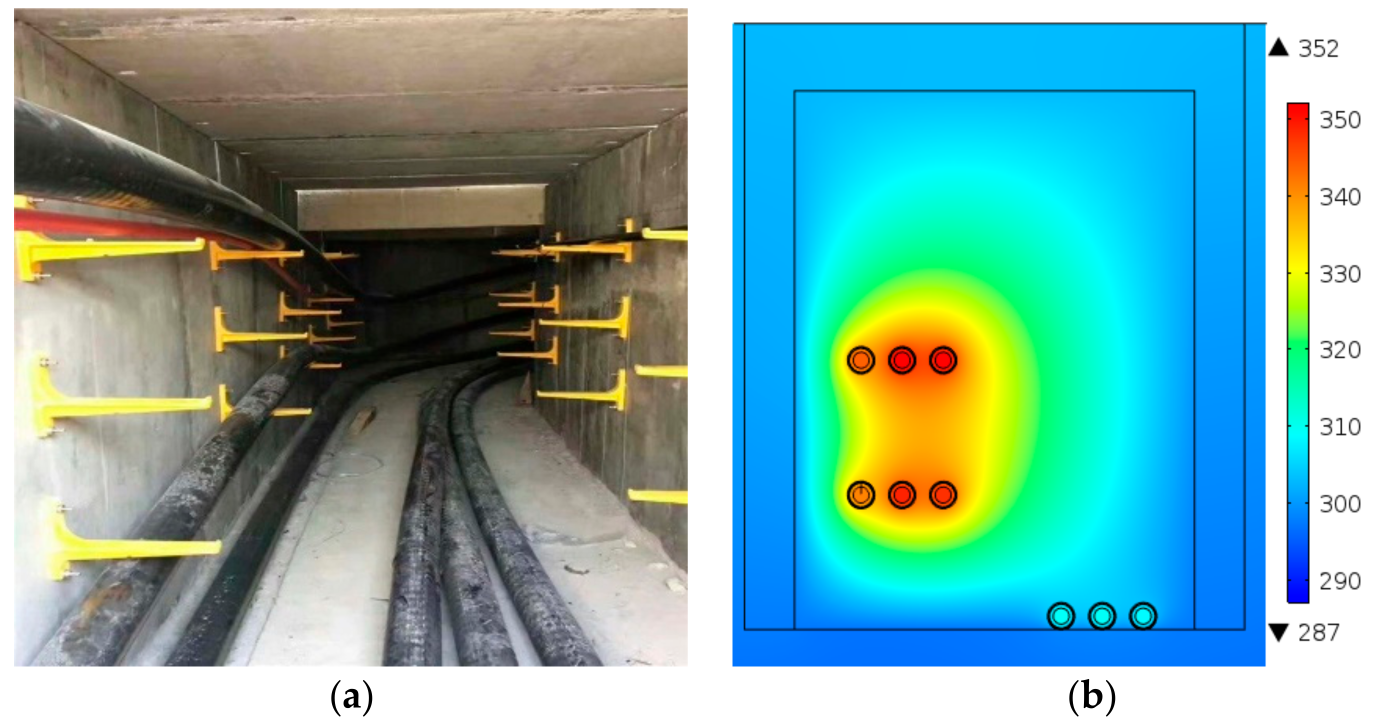
In fact, it is common that cables are laid irregularly in the actual cable trench of urban power grid, and the temperature distribution and carrying capacity of the cable trench are rarely studied. At the same time, there is almost no comparative study between IEC60287 and numerical calculation methods.
In this article, two methods are used to calculate the temperature of cable core, and a comparative analysis is made. The temperature distribution and cable ampacity of irregular distribution cable trench is studied. At the same time, an online monitoring system is designed to monitor the condition of cable trench in real-time.

2. Calculation Principle and Comparative Analysis

2.1. Physical and Environmental Parameters

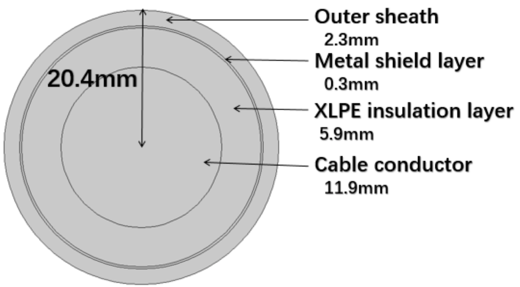
The single-core cross-linked polyethylene (XLPE) low-voltage cable of 8.7/15 kV YJV 1 × 400 is taken as the research object, and its main structure is shown in Figure 1.
The cable structure parameters and environmental parameters are shown in Table 1 and Table 2.

2.2. IEC-60287 Thermal Circuit Method

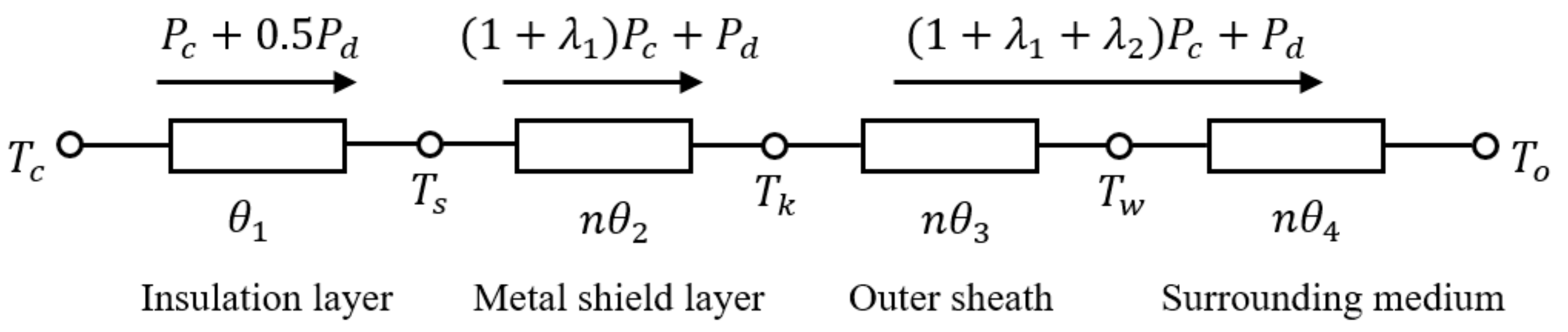
IEC-60287 is a common analytical method for calculating core temperature and cable ampacity. This method obtains the temperature distribution of different layers of cables by solving the equivalent thermal circuit, calculating the power loss of cables and the thermal resistance of the surrounding environment. The equivalent thermal path of the cable and its surrounding environment is shown in Figure 2.
By thermal path model.
T c = T 0 + ( P c + 0.5 P d ) · θ 1 + [ ( 1 + λ 1 ) P c + P d ] · n θ 2 + [ ( 1 + λ 1 + λ 2 ) P c + P d ] · n ( θ 3 + θ 4 )
where
P c = I 2 R , P c is the power loss of the cable conductor per unit length, W / m .
I is the current effective value of the cable conductor, A .
R is the AC resistance of the cable conductor at the highest temperature, Ω / m .
P d is the power loss of cable insulation layer per unit length, W / m .
λ 1 and λ 2 are the loss coefficient of metal shield layer and the armor layer, respectively, constant without unit.
θ 1 , θ 2 , θ 3 , and θ 4 represent the thermal resistance of insulation layer, metal shield layer, outer shield layer, and surrounding medium, respectively.
n is the number of cable cores, for single-core cable, n = 1 .
T c and T o represent the temperature of the core and skin temperature of the cable, respectively, K .
The cables studied in this article are single core cables. The thermal resistance and power loss in Equation (1) are calculated by the formula from IEC standard. The skin temperature of the cable is obtained by Equation (1), and then the conductor temperature of the cable is calculated too.

2.3. Numerical Calculation Method

2.3.1. Model of Cable Trench

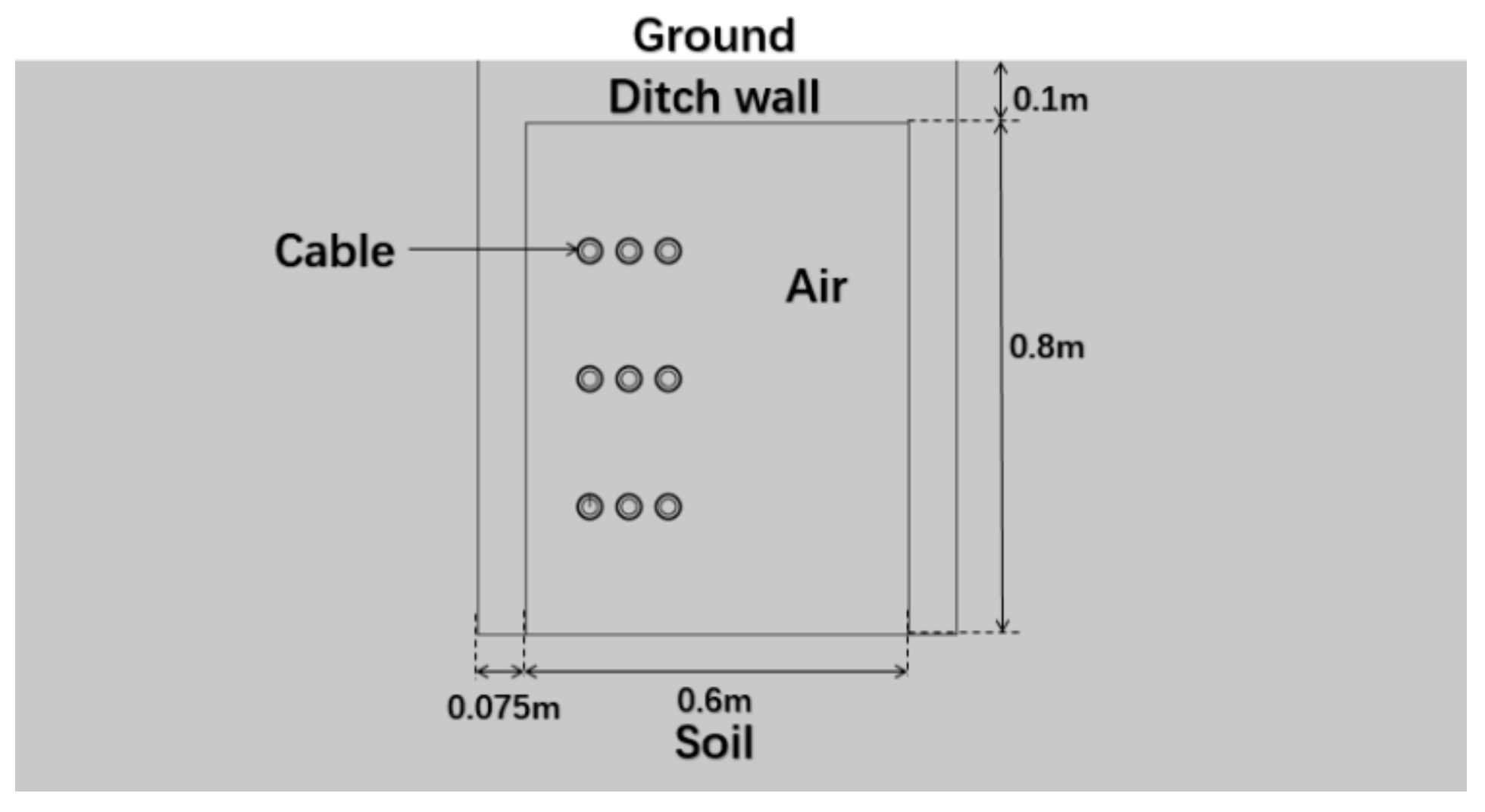
We assume that the length of the cable is infinite corresponding to its cross-sectional area. In addition, in steady state operation, there is almost no temperature gradient along the cable axis. Therefore, the two-dimensional model can reflect the temperature distribution of cable trench. Because the influence of angle steel brackets is small, they are neglected in the two-dimensional model. Therefore, the two-dimensional model as the cross-section of the cable trench shown in Figure 3 looks like triple three-loop cables float in the trench.
The cross-sectional area of inner cable trench is 0.6 m*0.8 m. Cable trench wall are 0.075 m thick, the lid is 0.1 m thick and the whole size including soil and trench is 3.15 m × 2.5 m. A total of nine cables are laid on angle steel brackets in three layers, and the current value of each phase cable is the same as 200 A, which is less than the cable ampacity. The ambient temperature is 293.15 K and the soil temperature is 287.15 K in the distance. The reference temperature is the initial temperature set by the COMSOL system, which is 293.15 K.
The following assumptions are made.
(1)
The steady state temperature field distribution of cable trench is simulated only.
(2)
The material properties of the cable and cable trench environments are all isotropic homogeneous media, and the physical properties of materials are constant.
(3)
Only the balanced operation of the cables is considered.
(4)
The metal shield or sheath layer of the cable is grounded at a single point, without considering the circulation loss of the shield layer.

2.3.2. Heat Transfer Equation

Simulating the steady-state temperature field of cable trench is a two-dimensional steady-state heat transfer problem. There are two different heat transfer equations including heat source or not:
(1)
The heat transfer differential equation of the area containing heat source (including cable core, insulating dielectric layer, and shielding layer) is as follows.
2 T x 2 + 2 T y 2 + q v λ = 0
T is the temperature at the point (x, y) in the domain, °C.
q v is the unit volume calorific rate, W / m 3 .
λ is thermal conductivity, W / ( m ° C ) .
(2)
The heat transfer differential equation of the area without heat source (including other cable layers, soil, cable trench wall, etc.) is as follows.
2 T x 2 + 2 T y 2 = 0

2.3.3. Boundary Condition

There are three main boundary conditions for heat transfer problems.
(1)
Constant boundary temperature.
{ 2 T x 2 + 2 T y 2 = 0 T ( x , y ) | Γ 1 = f ( x , y ) | Γ 1
(2)
Normal heat flow conditions with constant boundary normal heat flux density.
{ 2 T x 2 + 2 T y 2 = 0 λ T n | Γ + q 2 = 0
(3)
The convective heat transfer conditions in the interface between solid and fluid, occurring when the temperature of the fluid and the convective heat dissipation coefficient of the fluid are known.
{ 2 T x 2 + 2 T y 2 = 0 λ T n | Γ = α ( T T f ) | Γ
In the formula,
λ is the thermal conductivity, W / ( m · ° C ) .
f ( x , y ) is a temperature function on the boundary.
q 2 is heat flux density, W / m 2 .
α is convective heat transfer coefficient, W / ( m 2 °C).
T f is the fluid temperature, °C.
Γ and Γ 1 are the integral boundary.
According to the actual working environment of cable trench, the boundary conditions are determined as follows.
As shown in Figure 3, the temperature does not change in the horizontal direction of the boundary 1.2 m away from the cable trench, so the left and right boundaries of the model have a normal heat flow condition. The upper boundary is the ground plane, which is directly in contact with the air flow and meets the convective heat transfer conditions, and we take 25 °C as the air temperature. The lower boundary is deep soil, which can be regarded as a constant temperature boundary condition.
For direct buried cables, cable heat is commonly considered have no effect on soil 2 m outside. In addition, the soil 1 m away from the cable trench wall is not affected. Therefore, the boundary of rectangular solution domain was set as a line 1.2 m away from cable trench wall. Meanwhile, the upper boundary took the convective boundary condition.

2.4. Thermal Process Analysis of Cable Trench

Heat generation: In the whole solution area, only the cable produces heat, which comes from the Joule heat, dielectric power loss and induced power loss of the cable. AC resistance and inductance loss of multi-group single-core cables are calculated by analytical method according to IEC60287 standard.
Heat dissipation: The thermal process of cable trench includes heat conduction, convection and radiation. Specifically, the inner part of cable body, angle steel bracket, cable trench wall and soil mainly deliver heat through heat conduction. Natural heat convection and radiation mainly happen between solid and air in cable trench, they also happen between the upper cover of cable trench and surface air.

2.5. Results and Data Analysis

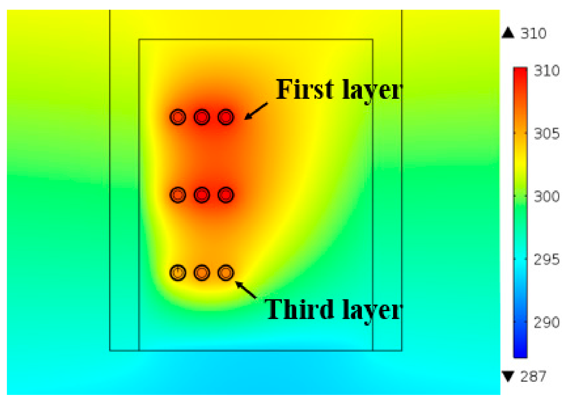
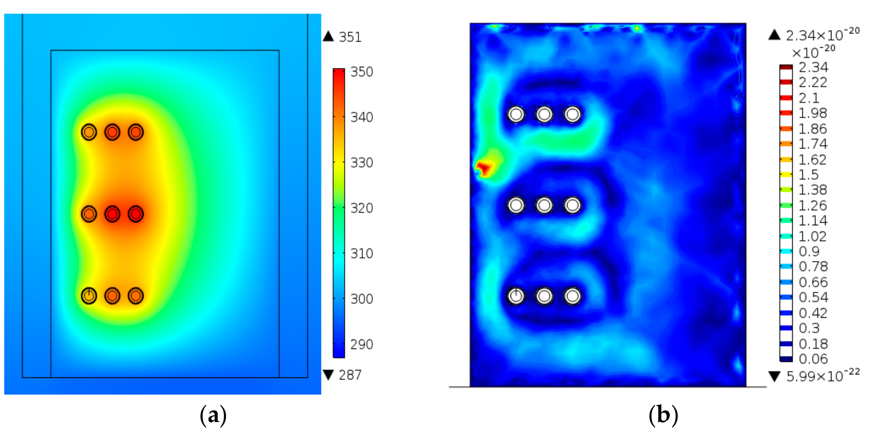
The temperature field distribution of the regularly laid cable trench is calculated, as shown in Figure 4.
It can be seen that the hottest part of the cable trench is around each cable group, and the hottest spot (310.28 K) appears at the core of the first layer cable. The lowest temperature in the cable trench is 298 K, which is basically consistent with the ambient temperature (293.15 K). The maximum temperature rise in the cable trench after thermal balance is as small as 20 K when operation current of the cable is not big enough. It can be found that the temperature of the upper cable is obviously higher than that of the bottom cable, which is due to the rise of hot air which causes the ambient temperature of the upper cable to be higher than that of the bottom cable.
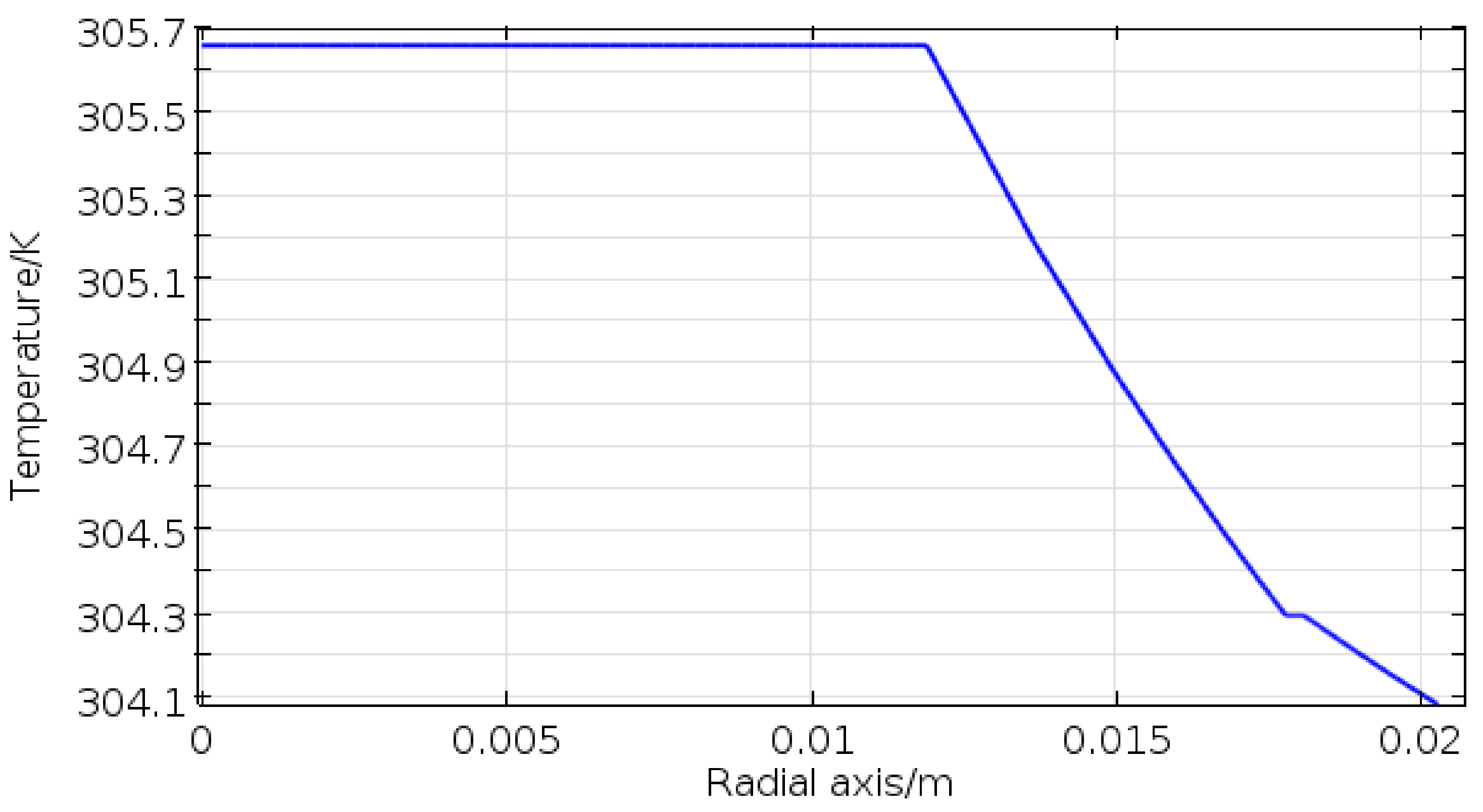
According to the results of by numerical calculation, the temperature variation trend from the cable skin to the core can be obtained, which makes it possible to calculate the core temperature value with measured temperature of outer layer. The temperature of cable core is studied by taking the cable of lowest layer and near the cable trench wall. The diagram of temperature value along cable radius is shown in Figure 1. The temperature variation along the radius of cable is shown in Figure 5.
We can see that the temperature of the cable core is 305.68 K and the temperature difference between cable core and skin is ~1.7 K. It is inferred that the thermal conductivity of cable insulation layer is quite low and its heat dissipation ability is weak, which leads to a slight decline in temperature along the insulation layer. The temperature changes along the metal shield layer and the outer shield layer of the cable tend to ease, and the temperature decreases slightly.
The temperature of cable core is calculated by thermal circuit method and numerical calculation method respectively, and compared with the field test value (as the standard values). When the current is 200 A, the temperature calculated by thermal circuit method and numerical calculation method is 319.20 K and 310.28 K, respectively, and the field test value is 311 K.
The relative error of temperature calculated by thermal circuit method is 2.3%, and that calculated by numerical calculation method is 0.32%. Obviously, the method of calculating cable core temperature by numerical calculation is closer to the true value.

3. Calculation of Cable Trench Temperature Field and Cable Ampacity

The XLPE power cable with three-loop cables of 8.7/15 kV YJV 1 × 400 is simulated by Multiphysics software.

3.1. Cable Ampacity Calculation Method

Secant method is used to determine the temperature value of cable conductor. It has super linear convergence and requires two initial solutions. The solution formula is
x k + 1 = x k f ( x k x k 1 ) f ( x k ) f ( x k 1 )
x k is current value. f ( x k ) is temperature function. The condition to terminate the algorithm is | f ( x k ) 90 | < k , k is the threshold value, and the temperature is taken as 1 °C in this article. The calculation steps of secant method are as follows.
(1)
To estimate the current according to the operation condition, we take the estimated value as the first current tentative value x k 1 , then f ( x k 1 ) is calculated. If f ( x k 1 ) meets the condition, then x k is the cable ampacity. Otherwise, turn to step (2).
(2)
The second current test value x k , which is not much different from the estimated value, is selected to calculate f ( x k ) . If f ( x k ) meets the condition, then x k is the cable ampacity, otherwise, turn to step (3).
(3)
We take f ( x k 1 ) and f ( x k ) into formula (7) to get x k + 1 and calculate f ( x k + 1 ) . If f ( x k + 1 ) meets the condition, then x k + 1 is the cable ampacity. Otherwise, turn to step (4).
(4)
x k 1 = x k , f ( x k 1 ) = f ( x k ) , x k = x k + 1 , f ( x k ) = f ( x k + 1 ) , turn to step (3).
Because the permissible working temperature of XLPE cable is 90 °C for a long time, the above f ( x k 1 ) ,   f ( x k ) ,   and   f ( x k + 1 ) are calculated according to currents x k 1 ,   x k ,   and   x k + 1 , respectively, and the operating temperature of XLPE cable is calculated by finite element method.

3.2. The Simulation of Temperature Field Distribution

Two laying modes of cables are compared as below.

3.2.1. Regular Laying Cables

The temperature field distribution of regularly laid cables with 200 A is simulated as shown in Figure 4 and the air flow field distribution as shown in Figure 6.
It can be seen from Figure 6 that the air flow rate in the cable trench is very slow, on the order of 10−22 m/s, because the trench lid is normally closed. Therefore, we may think that the air in the cable trench is still. The natural convection, or heat dissipation, of air has little contribution to heat transfer, and heat conduction is main factor. However, the air flow velocity near the cable on the left side of the cable trench is slightly faster than that in other areas, which may be due to the large temperature difference near the heat source, resulting in the acceleration of air flow velocity.
According to Equation (7), cable current ampacity is 481 A when the three-loop cables were laid regularly. The temperature field of the cable trench with this maximum current per phase is simulated in Figure 7a, and the air velocity field is shown in Figure 7b. In this situation, the cable maximum temperature is 351 K, which is the permissible temperature for long-term operation of XLPE cables, considering the temperature rise is as big as 53 K. There is no significant difference about the regularity of temperature field and air velocity field of cable trench comparing 481 A and 200 A. The highest temperature area is still concentrated around the cable, and the maximum temperature is 350.80 K.
Nine cables are numbered: the first layer is labeled 1, 2, and 3 from left to right. They are labeled in turn. The core temperatures are listed in Table 3.
Obviously, the temperature of the first layer cable is the highest when the current is 200 A, but the temperature of the middle layer cable is the highest when the current reaches the cable ampacity. The reason may be that when the current is large, a large amount of heat cannot be released to the outside world, which makes the air temperature in the middle layer of the cable the highest.

3.2.2. Irregular Laying Cables

Frankly speaking, the cable is often laid irregularly. It is necessary to focus on the temperature difference between laid in regular and laid in irregular. We list two cases as follows.
The calculation results show that the cable ampacity is decreased 87.5% from 481 A to 420 A according to Equation (7). One case, all the triple-loop cables are laid at the bottom of the cable trench. The corresponding temperature field of cable trench is shown in Figure 8a, and the velocity distribution of air flow field in cable trench is shown in Figure 8b.
The main reasons are as follows. (1) All cables are gathered at the bottom of the cable trench. The higher density arrangement reduces the convective heat transfer intensity between cable and air. (2) Intensive laying can enhance the induction effect among the cables, which results in increased heat production, higher temperature, and smaller cable ampacity. Although the air flow rate on the right side of the cable trench without the angle steel bracket is relatively fast, it can still be regarded as seldom air flow, and the heat dissipation effect of natural convection is very weak.
In the second case, where only one of the three layers of cables on the angle steel bracket is laid at the bottom of cable trench, it is assumed that the external environment and the position of the cables laid at the bottom remain the same. When the first layer cable is laid at the bottom of the cable trench the current ampacity is 517 A according to Equation (7); photos on-site and temperature field distribution are shown in Figure 9. The cable ampacities calculated from each laying situation are shown in Table 4.
Table 4 shows that there is no significant difference in cable ampacity, comparing 517 A to 513 A, when the first and third layers of cables are laid at the bottom of the cable trench. However, when the second layer cable is laid at the bottom, the cable ampacity increases to 542 A. Having the second layer laying at the bottom leads to the lowest degree of cable density, which may be the reason for the largest cable ampacity value. Under standard regular laying, the current carrying capacity of the cable is only 481 A, which means laying the cable in layers at the bottom of the cable trench can increase the cable ampacity, but it may lead to cable immersion, so this scheme is not recommended. The maximum value of temperature in Figure 7a and Figure 9b is basically the same. But when the current reaches the cable ampacity, the highest temperature point of the regular laying method is in the middle layer cable, while the highest temperature point of Figure 9b is in the third layer cable.
By comparison, it can be concluded that increasing the spacing between cable groups is helpful for heat dissipation and the cable ampacity. But it increases the space and construction cost of cable trench, so both should be taken into account when designing cable trench.

4. Online Monitoring System

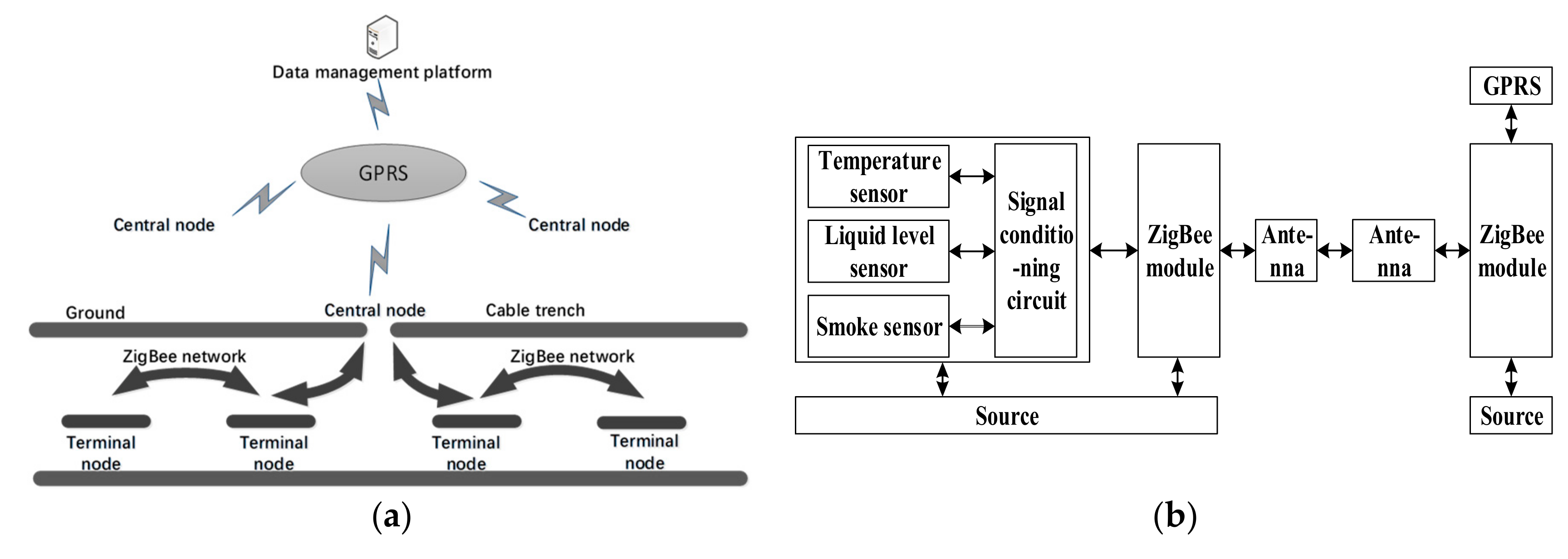
4.1. System Overview

An online monitoring and prewarning system for cable trench was developed to acquire data such as cable temperature, water level of trench and smoke concentration. The scheme design and data flow chart of the monitoring system is shown in Figure 10a, and the structure of hardware modules is shown in Figure 10b.
The monitoring unit includes all kinds of sensor module, data acquisition module, and ZigBee wireless transmission module. The terminal node collects the temperature of cable body, joint, water level and smoke concentration respectively. The central node is installed at the outlet of cable trench, including ZigBee receiving module, General packet radio service (GPRS) transmitting module and source. Finally, a polling method is used to read the data of the terminal nodes.
GPRS transmitter module upload data to data acquisition terminal. ZigBee module has the advantages of low power consumption, low-cost, big network capacity, and enough communication distance in cable trench. So it is used for temperature data acquisition, conditioning, and data transmission between nodes. The received node data is sent to the mobile phone through GPRS by serial communication. The system consists of Zigbee coordinator and terminal nodes. The core device is the coordinator node, it establishes, initializes, and configures the network, receives and processes information from terminal nodes, and then transmits information to remote monitoring mobile phone through GPRS, namely, to fulfill real-time data sending and receiving. The data management platform has the function of receiving and analyzing data, and uses the numerical method described above to calculate the temperature of cable core quickly, accurately.

4.2. Program Design and Implementation of Monitoring System

After power-on initialization, the coordinator chooses the appropriate channel to build up its own new network, which includes the setting of PANID, the generation of short address of the coordinator and so on. Then, in the event handler function of coordinator uint16SampleApp_ProcessEvent (uint8 task_id, uint16 events), the data packet is received by calling the subfunction SampleApp_MessageMSGCB (MSGpkt). The terminal node sends the incoming signal to the coordinator to join the network. Uint16, SampleApp_ProcessEvent (uint8 task_id, uint16 events), registers events, sets numbers, send times, and so on. After setting, the function SampleApp_SendPeriodicMessage() is called to broadcast the sensor data periodically.

4.3. System Performance Testing

The infrared temperature sensor of the online monitoring system is installed aiming at the point of highest temperature of the cable obtained by the simulation. The maximum long-term permissible operating temperature of XLPE insulated cable is 90 °C, so that 90 °C was set as the temperature warning threshold of power cable. Model S20-3 infrared thermometer was selected as temperature sensor. The acquisition accuracy is 0.1 °C, which can meet the measurement accuracy requirements. The surface temperature of the object can be calculated by measuring the infrared radiation intensity emitted by the target without touching or injecting the cable. In order to test the sensitivity and accuracy of the temperature, acquisition experiments were done many times, taking a thermostatic plate as the test object. The actual temperature of the thermostatic plate was measured by a thermometer at the same time. The data are shown in Table 5 below.
Table 5 shows that the maximum relative error of the test results is 2.54%, which can meet the requirement of accuracy value as 1 °C.

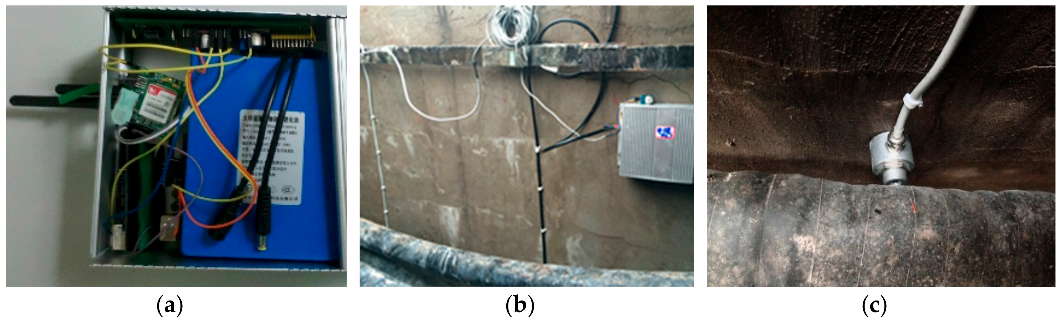
4.4. Application of Monitoring System

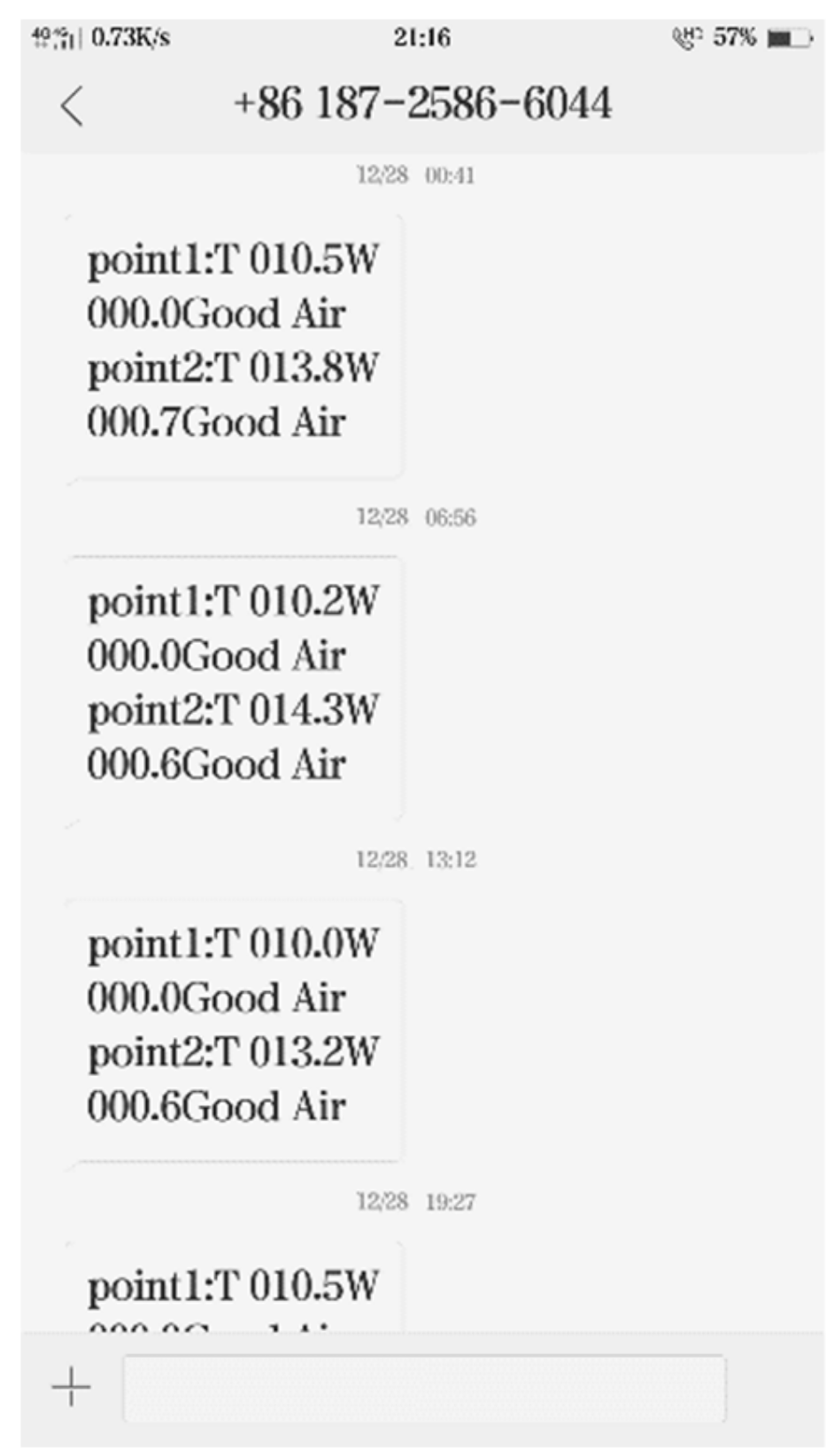
The online monitoring system has been installed in Nan’an Power Supply Bureau of Chongqing for trial operation. The highest temperature of cable trench is obtained by simulation analysis. Temperature sensors are arranged at the highest temperature to obtain the highest temperature inside the cable trench, so as to ensure that the overall temperature of cable trench does not exceed the specified value. The two temperature measurement points represented by node 1 and node 2 are located nearby the cable connector and the body of cable conductor, respectively. The distance between the two points is ~20 m. The sampling frequency of the system is every 20 s, and the response time of the infrared thermometer is 100 ms. If extremely high temperature or thick smoke occurs in the cable trench, the monitoring system will send an alarm message timely. If the cable trench runs normally, the monitoring system will send status information, including temperature and air conditions, to the mobile phone almost every 6 h and store them as historical data. On-site photos of the monitoring system are shown in Figure 11a–c. Information sent by GPRS are shown in Figure 12 and also listed in Table 6.
Because the cable trench environment is relatively closed, the main determinants of temperature are load conditions and the surrounding environment of the cable. Table 6 shows that the temperature value of both node 1 and node 2 is only a little bit bigger than 10 °C at ambient temperature, which indicates that the cable works normal with quite small load current. Meanwhile, the temperature of the cable joint is slightly lower than that of the cable skin. The reason may be that the package is thicker at the cable joint. The temperature of cable skin varies within the normal range, and the temperature distribution versus time is not uniform, but has certain regularity, which is consistent with the various load. In general, the monitoring system runs well and the data transmission works reliably.

5. Discussion

With the development of urban power grid, the number of power cables with various voltage levels is increasing, and the laying modes of cables are becoming more and more complex. Current research has done a lot of analysis on regular laying cable trench, but lack of research on irregular laying cable trench. Moreover, online monitoring cable trench can effectively warn early for the abnormal operation and prevent from electrical accidents. We have conducted the following research works to meet the requirements mentioned above.
(1)
For regular laying cable trenches, the simulated temperature field distribution with different structures has been proposed by many existing literatures, but the simulation error is relatively large, or the overall temperature field inside cable trenches has not been showed, only the temperature distribution curves of a row of cables were given. In this paper, the cable body temperature is obtained by IEC60287 thermal circuit method and numerical calculation method, the error is 0.32%, which can fully meet the actual requirements of the project. In addition, the temperature field and velocity field of the whole cable trench are analyzed.
(2)
For irregularly laying cable trenches, few reports can be found in the existing literature. However, the irregular laying of cables is common in field, which may lead to unstable operation and even causes fire in cable trenches. In this paper, the conclusion about both simulation analyses of irregularly laid cables and the calculation of cable current carrying capacity are helpful to standardize the construction of cables.
(3)
An online monitoring system is developed to detect timely the highest temperature of cables through simulation analysis, which effectively reduce the number of sensors. Infrared temperature sensors and zigbee are applied with low cost and easy to be installed.
Research work above is of great significance for the safety of urban power system and the improvement of its stability and reliability.

6. Conclusions

This article compares the numerical calculation method with the thermal circuit method in calculating the steady-state temperature distribution of cables, and verifies the advantages and accuracy of the former method. The distribution of temperature field and cable ampacity under different cable laying situation are analyzed and compared. The main results are as follows.
(1)
Numerical calculation method is more accurate than traditional analytical method in calculating the temperature of cable core based on the temperature of cable skin. The relative error of numerical method is 0.32% and that of the analytical method is 2.3%.
(2)
According to the result of steady-state temperature field simulation for the triple-loop cable trench, when the current is small, the hottest point is the core of the first layer cable, and when the current is large, the highest temperature is in the middle layer cable.
(3)
Cable laying mode greatly affects the cable ampacity. When the cable cluster is laid at the bottom, the cable ampacity is less than that of regular three-layer cables. The regular mode can reduce the working temperature and prolong the service life of the cable. The higher the density of the cable cluster, the lower the cable ampacity.
(4)
An online monitoring system for working environment of power cable is developed. It monitors the temperature of cable, water level in ditch and smoke concentration comprehensively, as to warn faults quickly.

Author Contributions

Conceptualization, L.X. and Y.C.; Formal analysis, L.X.; Methodology, L.X.; Software, Y.C.; Validation, Y.J., J.W., and X.H.; Writing—original draft, Y.C.; Writing—review & editing, L.X.

Funding

This research was supported by the Chongqing Nan’an Branch Company of the State Grid of China.

Conflicts of Interest

The authors declare no conflicts of interest.

References

  1. International Electro Technical Commission. IEC 60287-1. Calculation of Current Rating Part 1: (100% Load Factor) and Calculation of Losses; IEC: Geneva, Switzerland, 2001. [Google Scholar]
  2. Shen, M. Numerical analysis of temperature field in a thawing embankment in per. Can. Geotech. J. 2011, 25, 163–166. [Google Scholar] [CrossRef]
  3. Lianghua, Z.; Jianjian, Y.; Xiaohu, Z.; Zhiwei, L. A new method for calculating the current carrying capacity and steady-state temperature field of directly buried cables. High Volt. Technol. 2010, 11, 2833–2837. [Google Scholar]
  4. Yongchun, L.; Yanming, L.; Jinai, C.; Zhenggang, W.; Zhongkui, L. A new method for calculating steady-state temperature field and carrying capacity of underground cable group. J. Electr. Technol. 2007, 22, 185–190. [Google Scholar]
  5. Youyuan, W.; Rengang, C.; Weigen, C.; Jin, T.; Yuan, Y. Cable current carrying capacity calculation under cable trench laying mode and its influencing factors analysis. Power Autom. Equip. 2010, 30, 24–28. [Google Scholar]
  6. Ruan, J.; Zhan, Q.; Tang, L.; Tang, K. Real-Time Temperature Estimation of Three-Core Medium-Voltage Cable Joint Based on Support Vector Regression. Energies 2018, 11, 1405. [Google Scholar] [CrossRef]
  7. Anders, G.J.; Napieralski, A.K.; Kulesza, Z. Calculation of the internal thermal resistance and ampacity of 3-core screened cables with fillers. IEEE Trans. Power Deliv. 1999, 14, 729–734. [Google Scholar] [CrossRef]
  8. Lee, S.J.; Sung, H.J.; Park, M.; Won, D.; Yoo, J.; Yang, H.S. Analysis of the Temperature Characteristics of Three-Phase Coaxial Superconducting Power Cable according to a Liquid Nitrogen Circulation Method for Real-Grid Application in Korea. Energies 2019, 12, 1740. [Google Scholar] [CrossRef]
  9. Sedaghat, A.; De Leon, F. Thermal Analysis of Power Cables in Free Air: Evaluation and Improvement of the IEC Standard Ampacity Calculations. IEEE Trans. Power Deliv. 2014, 29, 2306–2314. [Google Scholar] [CrossRef]
  10. Boshan, Z.; Qingzhu, W. Real-time Conductor’s Temperature Calculation of High Voltage Cable and Prediction 409 Probe of Ampacity. Electr. Eng. 2017, 3, 10–15. [Google Scholar]
  11. Anders, G.J.; Brakelmann, H. Rating of underground power cables with boundary temperature restrictions. IEEE Trans. Power Deliv. 2017, 33, 1895–1902. [Google Scholar] [CrossRef]
  12. Yongchun, L.; Yanming, L.; Yanmu, L.; Zhenggang, W.; Zhongkui, L. Numerical methods for transient temperature field and short-term current carrying capacity of underground cables. J. Electr. Technol. 2009, 24, 34–38. [Google Scholar]
  13. Youyuan, W.; Rengang, C.; Weigen, C.; Jin, T.; Yuan, Y. Finite element method for calculating steady-state temperature field of underground cables and its influencing factors. High Volt. Technol. 2009, 12, 3086–3092. [Google Scholar]
  14. Yildiz, Ş.; İnanir, F.; Çiçek, A.; Gömöry, F. Numerical study of AC loss of two-layer HTS power transmission cables composed of coated conductors with a ferromagnetic substrate. Turk. J. Electr. Eng. Comput. Sci. 2017, 25, 3528–3539. [Google Scholar] [CrossRef]
  15. Garrido, C.; Otero, A.F.; Cidras, J. Theoretical model to calculate steady-state and transient ampacity and temperature in buried cables. IEEE Trans. Power Deliv. 2003, 18, 667–678. [Google Scholar] [CrossRef]
  16. Doukas, D.I.; Chrysochos, A.I.; Papadopoulos, T.A.; Labridis, D.P.; Harnefors, L.; Velotto, G. Volume element method for thermal analysis of superconducting DC transmission cable. IEEE Trans. Appl. Supercond. 2017, 27, 1–8. [Google Scholar] [CrossRef]
  17. Haiqing, N.; Wenjian, Z.; Chaoping, L.; Kaifa, Y.; Yong, W.; Guojun, L. Estimation method of soil thermal parameters around cables based on finite element method and particle swarm optimization. High Volt. Technol. 2018, 44, 1557–1563. [Google Scholar]
  18. De Leon, F. Major factors affecting cable ampacity. In Proceedings of the 2006 IEEE Power Engineering Society General Meeting, Montreal, QC, Canada, 18–22 May 2006. [Google Scholar]
  19. Bates, C.; Malmedal, K.; Cain, D. Cable Ampacity Calculations: A Comparison of Methods. IEEE Trans. Ind. Appl. 2016, 52, 112–118. [Google Scholar] [CrossRef]
  20. Shabagin, E.; Heidt, C.; Strauß, S.; Grohmann, S. Modelling of 3D temperature profiles and pressure drop in concentric three-phase HTS power cables. Cryogenics 2017, 81, 24–32. [Google Scholar] [CrossRef]
Figure 1. Schematic diagram of power cable structure.
Energies 12 03397 g001
Figure 2. Thermal path model of the cable.
Energies 12 03397 g002
Figure 3. Two-dimensional geometric model of cable trench with triple three-loop cables.
Energies 12 03397 g003
Figure 4. Temperature field distribution in cable trench (unit: K).
Energies 12 03397 g004
Figure 5. Temperature curve along radial direction of cable.
Energies 12 03397 g005
Figure 6. Air flow field distribution (unit: m/s).
Energies 12 03397 g006
Figure 7. Temperature field and velocity distribution in trench with cable current ampacity of 481 A. (a) Temperature field distribution (Unit: K). (b) Air flow field velocity distribution (unit: m/s).
Energies 12 03397 g007
Figure 8. Temperature field and velocity distribution with 420 A current. (a) Temperature field distribution (Unit: K). (b) Air flow field velocity distribution (unit: m/s).
Energies 12 03397 g008
Figure 9. Photos on site and temperature field distribution with 517 A current. (a) Photos of cables irregularly laid on site. (b) Temperature field distribution (Unit: K).
Energies 12 03397 g009
Figure 10. Overall scheme and function module of online monitoring system. (a) Scheme and data flow chart. (b) Functional modules and structures.
Energies 12 03397 g010
Figure 11. Online monitoring system. (a) Internal structure, (b) installation appearance of monitoring system, and (c) temperature sensor.
Energies 12 03397 g011
Figure 12. Information sent by GPRS.
Energies 12 03397 g012
Table 1. Parameters of cable structure.
Cable Structuremm
Inner radius of cable11.9
Insulation width5.9
Metal shield width0.3
Outer sheath width2.3
Outer radius of cable 20.4
Table 2. Environmental parameters of cable trench.
Laying EnvironmentParameter Values
Soil thermal resistance/ K · m · W 1 23.8
Air temperature/ K 313
Deep soil temperature/ K 293
Ditch wall thermal conductivity/ W / m · K 1.73
Bracket thermal conductivity/ W / m · K 44.5
Table 3. Temperature of cable cores.
Cable Serial Number200 A/K481 A/K
1308.66338.54
2310.28345.48
3310.16344.77
4308.08342.43
5309.98350.80
6309.92350.60
7305.68335.44
8306.42342.31
9306.42341.49
Table 4. Cable ampacity when different layers are laid at the bottom.
Cables at the BottomCable Ampacity/A
First layer517
Second layer542
Third layer513
Table 5. Temperature test data.
Test PointActual Value/°CTest Value/°CRelative Error/%
Node 220.220.61.98
Node 220.821.21.92
Node 221.521.91.86
Node 228.228.82.12
Node 228.528.91.40
Node 224.825.21.61
Node 224.424.92.04
Node 223.624.22.54
Node 223.523.91.70
Node 223.523.91.70
Table 6. Temperature data monitored.
Test PointTimeTemperature (°C)
Node 100:4110.5
06:5610.2
13:1210.0
Node 200:4113.8
06:5614.3
13:1213.2

