1. Introduction
With environmental concerns of fossil-fuel-based energy consumption, renewable energy has been playing a predominant role in clean and cost-efficient energy production, contributing significantly to the sustainability of human society. One of these renewable energy sources is the large-scale wind turbines with a doubly-fed induction generator (DFIG), which have been widely installed attributing to their low lifecycle costs. In a DFIG wind turbine system, the gearbox plays an important role in the drive train of a wind turbine. However, due to the variable heavy load from turbulent wind and other uncertain factors, gears usually suffer unbalanced and varying loads, which results in dramatic temperature rising and viscosity reduction in the lubricant. As a result, gears might be gradually deteriorated. These faults take the responsibility of unexpected system breakdown and extra expenditures on turbine maintenance [
1]. Therefore, fault diagnosis and forecasting are of great importance to the resilience of turbine systems and reduction of maintenance costs. Over the years, a significant body of studies has been conducted targeting the troubleshooting of wind turbine systems. Chen et al. proposed an empirical wavelet transform method for fault diagnosis in wind turbine generator bearing fault diagnosis and found that this method can enhance performance in the weak feature detection of wind turbine drivetrain [
2]. Biswal et al. utilized vibration analysis for wind turbine fault diagnosis and conclude that the fault size for gear root cracks could be identified successfully [
3]. Moreover, Zhang et al. employed acoustic emission signals for wind turbine gearbox fault diagnosis, as expected, found that the locations of faults can then be determined [
4]. The literature review indicates that most of those fault diagnosis methods are based on vibration and acoustic signals, however, vibration signals monitored with additional vibration sensors and equipment will result in extra investment on maintenance, as well as the increase of computational load and difficulty in signal processing.
As to the fault detection and prediction of key components in turbines, recent advances in sensors and signal processing have been contributing significantly to the monitoring and prognosis of WT gearboxes. However, accurate fault detection and reliable diagnosis in wind turbine gearboxes are still challenging due to the inherited complexities in mechanical systems and operation conditions [
5]. Thus, more accurate and cost-efficient online monitoring is of essential importance on troubleshooting and enhancement of turbine system resilience. An effective condition monitoring might either evaluates component health conditions or helps with the detection and prediction of marginal changes that indicate incipient faults [
6]. The WT SCADA system with key parameters can be easily measured and monitored, including bearing and lubricant temperatures, rotor speed, environment temperature, and active power. Besides, it can continuously record the historical and present status of a wind turbine system.
The literature review also shows some successful studies in predicting faults caused by complex nonlinearity reasons using operational SCADA data combined with diverse approaches such as adaptive neuron-fuzzy interference systems (ANFIS), Bayesian Networks and Deep Learning Networks [
7,
8,
9]. A hybrid stochastic technique is proposed in reference [
10], which is based on an augmented observer combined with Eigen structure assignment for the parameterization and the genetic algorithm (GA) optimization to address the attenuation of uncertainty mostly generated by disturbances. Data mining techniques are also applied to this data combination to model the power curve [
11]. The results of reference [
12] demonstrate that the proposed method can effectively analyze nonlinear data trends, continuously monitor the WT and reliably detect abnormal problems by using six process parameters. An exponentially weighted moving average (EWMA) control chart was proposed in reference [
13] and used in Statistical Process Control to determine if the process is out of control. Wang et al. also presented a deep auto-encoder (DAE) method for anomaly detection and fault analysis of wind turbine components [
14]. Although some successful applications have been achieved, the limitations of the mentioned approaches cannot be overlooked. Firstly, it is difficult to process and interpret a large body of data collected from the SCADA system simultaneously. Secondly, conventional artificial intelligent techniques are inefficient in the extraction of features from raw data [
15]. Thirdly, the potential of the SCADA data might have not been fully explored [
16]. In this study, an algorithmic-level online WT fault detection method based on SCADA data using support vector regression (SVR) is proposed. The employed SVR algorithm, which is based on statistical learning and structural risk minimization is a nonlinear generalization of the Generalized Portrait algorithm developed in 1964 [
17,
18].
In light of the above, this research is established with the following operations. Firstly, in the case of decreasing structural risk, SVR can maximally excavate the implicit classification knowledge in the SCADA data. Secondly, as the number of faulty samples is relatively smaller compared with the number of right samples, SVR can address the imbalanced data issue. Thirdly, SVR can address the nonlinear system in fault diagnosis. In the developed SVR approach, SCADA data will be preprocessed and divided into two groups. The first group termed as “Training Data” is used to obtain the optimization function with the “soft margin”, which allows some “”. The second group termed as “Test Data” is then employed to validate the model performance. Once the measured data exceeds the confidential range, a developing fault then can be spotted.
To present the proposed methodology in a logic manner, the rest of this paper is organized as follows: the developed methodology is introduced in
Section 2, followed by the statistic control methods demonstrated.
Section 3 is focused on the development of an SVR model for wind turbine gearbox systems using 45 SCADA parameters. After that, a case study is employed to demonstrate and validate the established system in
Section 4. Finally,
Section 5 draws to concluding remarks and recommendations for future studies.
2. Methodology
Support vector machines (SVM), known as a kind of learning machine underpinned by the statistical learning theory, were firstly proposed by Vapnik et al. [
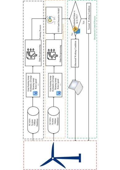
19]. Support vector regression (SVR) is a machine learning algorithm based on the principle of structural risk minimization is a common application form of SVMs. The SVR is a powerful function approximation technique of outstanding generalization performance, which can be used to obtain globally optimal solutions, as well as map a nonlinear regression problem into a linear regression problem by applying a kernel function. SCADA monitoring provides a series dataset including bearing and lubricant temperatures, rotor speed and active power. Compared to the condition monitoring based on vibration and acoustic signals, SCADA monitoring independent of additional sensors and previous fault datasets. However, raw SCADA data acquired from wind turbines requires precise mathematical modeling. And the mathematical model is sensitive to external disturbance. In addition, accurate modeling requires specification parameters and prior data under abnormal working conditions, which limited the application in diverse gearboxes under variable working conditions. Therefore, an SVR algorithm is developed in the research to explore the ability of self-study and disposal of complex nonlinearity. Moreover, only standardized real-time SCADA data is used in the construction of the SVR model to reduce the impacts of external disturbances. The methodology and framework of this study can be shown in
Figure 1.
To support the construction and optimization of the proposed SVR model, a grid search method based on cross-valid training data which is initially introduced in reference [
20], is employed for the SVR parameters optimization. After that, the temperature detection model of wind turbine gearboxes was setup, followed by the bearing and lubricate temperatures under normal working conditions were predicted. Then real-time data was fed into the SVR model for the calculation of the estimated residual. In order to detect the changes in online data, a moving average calculation was applied. Finally, the residual with distributing was operated in statistical process control. Once the residuals step out of the thresholds, incipient faults can then be predicted.
2.1. Support Vector Regression
SVM is a machine learning tool widely used in classification and regression analysis. The SVM regression is known as a nonparametric technique since it relies on kernel functions. Compared to other existing fault detection methods, the SVM is specialized in address problems with small sample size, nonlinear and high-dimensional datasets. Moreover, with the introduction of soft margin, the generalization ability of SVM is significantly enhanced. The initial design of SVM is to map the input vectors
into a higher dimensional feature space. Then the linear regression in this high dimensional space will be solved. The input space is defined by Kernel functions
[
21].
Given the training data
, where
denotes the total numbers of data and
demonstrate the values of independent variables or training data in this study.
is the output while
denotes the space of the input patterns (e.g.,
), one objective of this research is to find a function
that has at most
deviation from the actually obtained targets
for all the training data, and at the same time to set it as flat as possible. One of these functions is the Gaussian kernel, with the maximum tolerance of the deviation between
and
is
. By introducing a dual set of variables, the function then can be expressed as:
where the trade-off is determined by the constant
. The
loss function
in the context of deviations larger than
, can be described by
with the introduction of Lagrange multipliers, Equation (4) is then obtained.
In this equation, L is the Lagrangian and
,
,
,
are Lagrange multipliers. Hence the dual variables in Equation (5) have to satisfy the positivity constraints shown in Equation (5). Note that
refers to
and
here.
It follows from the saddle point condition that the partial derivatives of L with respect to the prime variables
must vanish for the optimality as shown.
By substituting Equations (6)–(8) into Equation (4), the dual optimization problem can then be obtained.
In deriving Equation (9) the dual variables
,
were eliminated through a condition Equation (8) which can be reformulated as
. Equation (7) can then be rewritten as
Thus, the SVR detection model can be expressed as
The complete algorithm can then be described in terms of dot products between the data acquired by the wind turbine SCADA system.
2.2. Statistic Control Methods
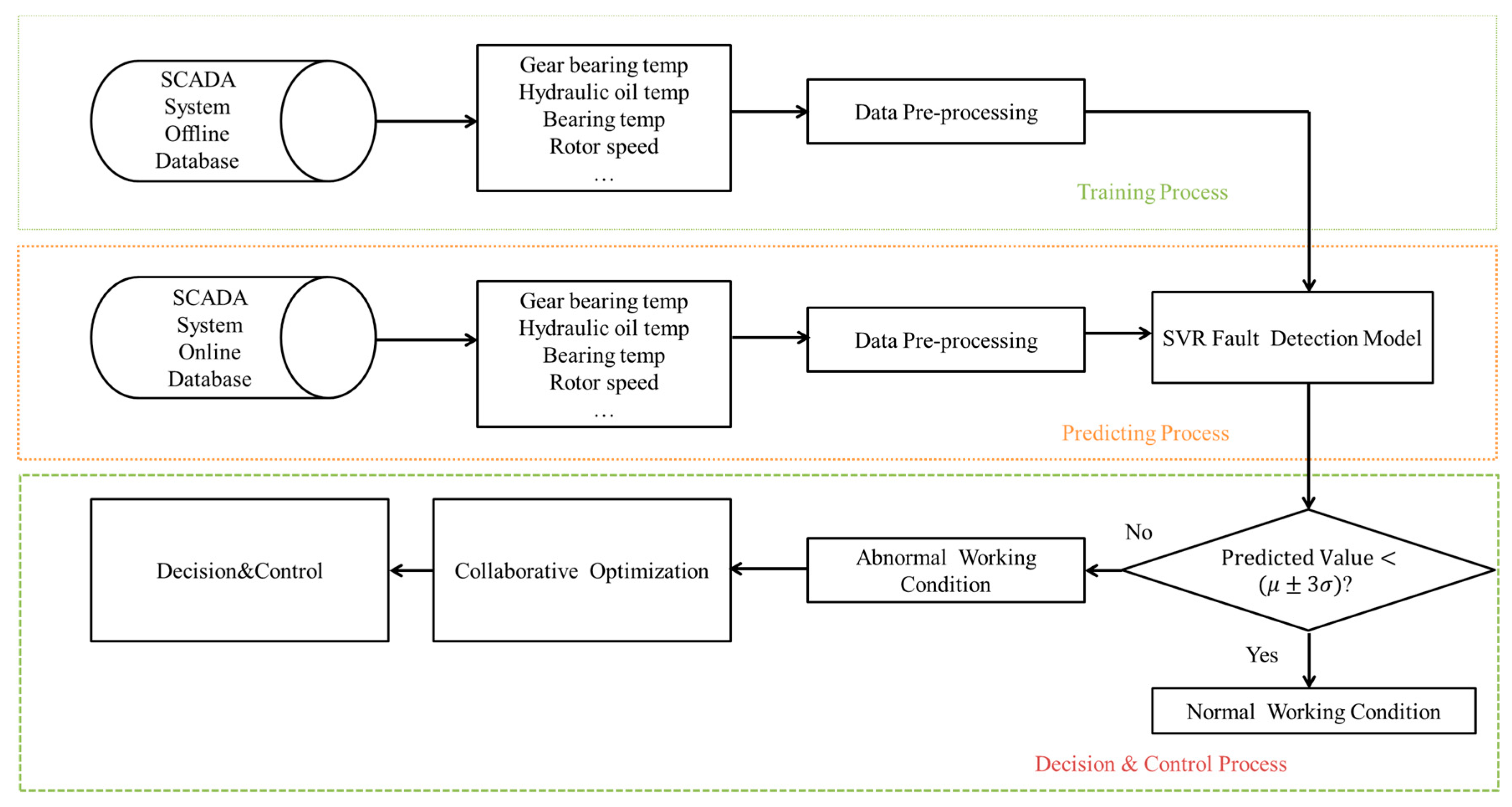
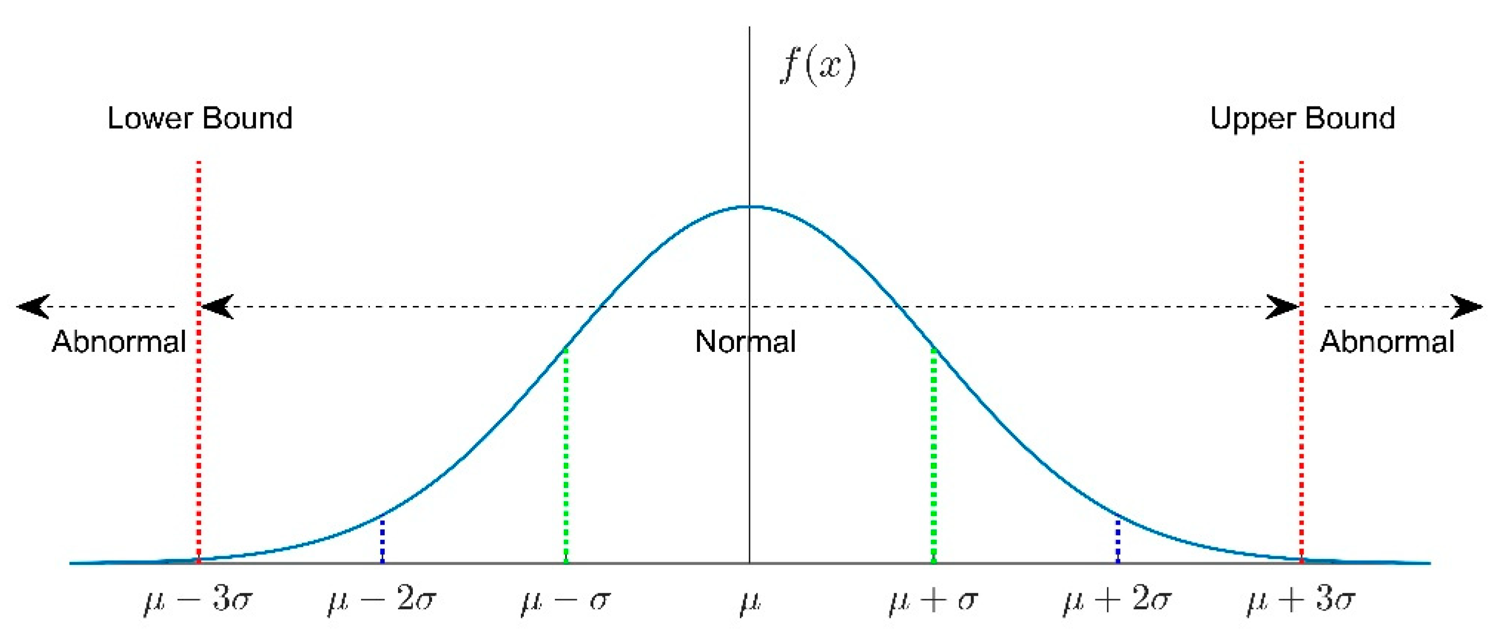
In order to identify if the wind turbine is working in normal, the statistic control method is applied to the time series of sample data. Mean, standard deviation, minimum and maximum of the data are collected within control limits. There are several rules to determine whether the data is out of control limits. In this study, the normal distribution was applied for the wind turbine SCADA data. Here, the normal distribution set up by central limit theorem as the distribution to which the mean value of almost any set of independent and randomly generated variables rapidly converges is an important class of statistical distributions.
The probability density function of the normal distribution is given as:
where
is the mean or expectation of the distribution,
is the standard deviation and
is the variance. Different values of
and
would produce different normal density curves and different normal distributions. The normal density can be specified by means of an equation. The probability distribution of a random variable
is identified to be normal if it has a probability density.
Figure 2 shows the changes in the normal distribution with the standard deviation. As shown in
Figure 2, 68% of the data falls in [
] standard deviation of the average, 95% of the data is within [
] the standard deviations of the average, while 99.7% of the data falls in [
] the standard deviations of the average. If the data is within [
], the process will be identified as working in normal. However, once the data goes beyond the control limits [
], the process will be considered as out of control, and then faults are detected.
3. Model Construction
3.1. Faults Detection Model of Wind Turbine Gearboxes
SVR is a detection algorithm based on statistical learning theory. The initial design of this algorithm is to minimize error, individualize the hyperplane and set a margin of tolerance. Analysis of the SCADA data in this study found that the values of parameters such as bearing temperature, lubricant temperature, and rotor speed are of high interactions.
The SVR detection model can be expressed as
where
and
denote the estimated values of bearing temperature and lubricate temperature.
is the bearing input.
is the temperature input. Note that
are previous sampling data of bearing temperature, lubricant temperature, environment temperature, rotor speed and active power at time
.
and
are historical sampling time of state variables.
and
is the kernel function of bearing temperature data and the lubricate temperature data. The Gaussian kernel is given as
where
is a given constant. One significant advantage of using Gaussian kernel is the possibility of operating in infinite dimension space, which results in that the feature space is easier to handle due to the linearity in feature space. Three of the parameters can be adjusted for setting an SVR with the Gaussian kernel, namely,
, and
. The SVR performance has a heavy dependence on the triplet of parameters. The parameter selection aligns with the value selection of the decision variables
, and
, which can maximize the SVR performance on test data. In SVR models, the number of data sets is measured by the sliding window N with N is further divided into 5 elements. After that, the optimal model parameters are obtained by using the fivefold cross-validation. Finally, the optimal model is used in online fault detection. In a 50% cross-validation, 40% of the sample is used for training and 10% of the sample is used for testing.
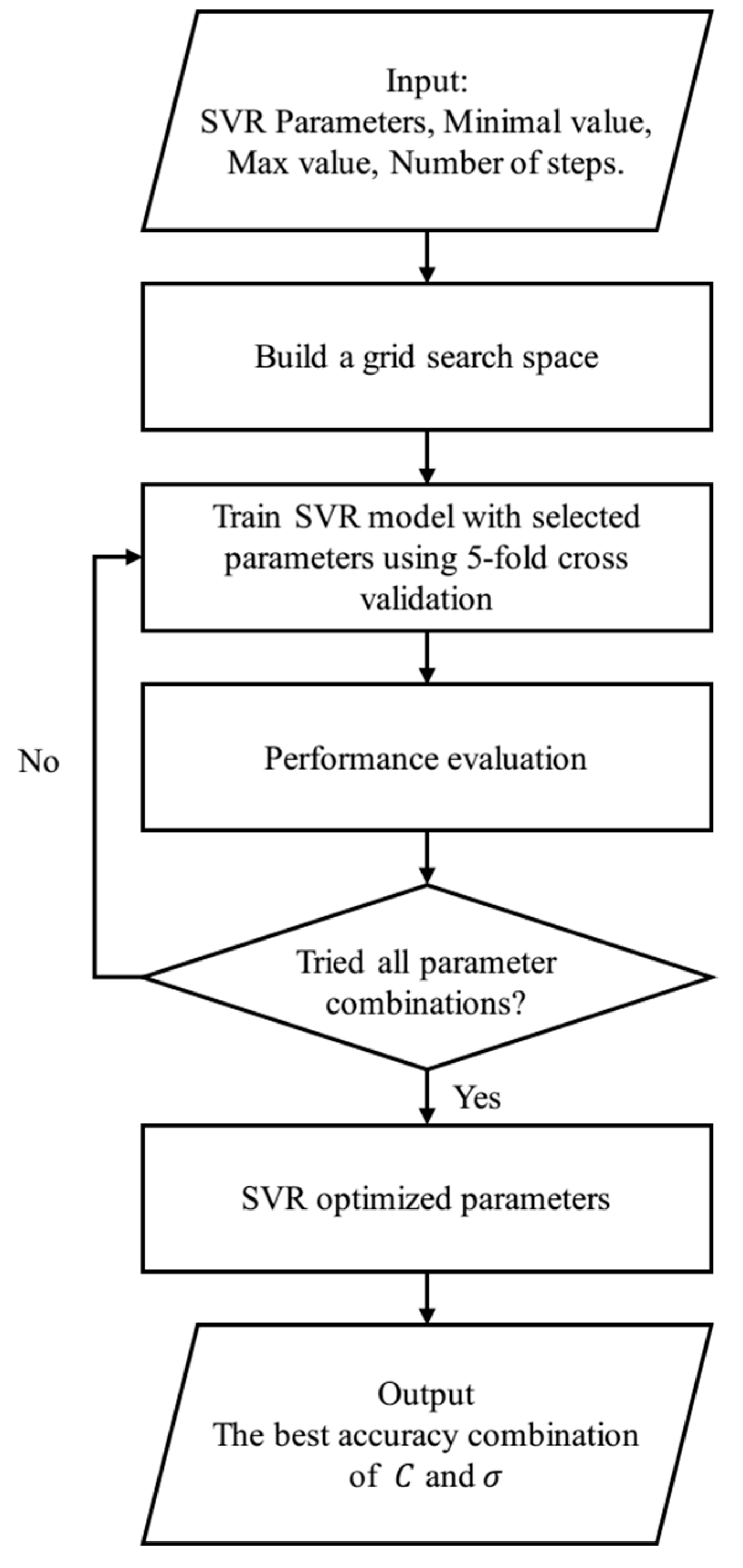
3.2. Experimental Setup and Procedure
As discussed in the previous section, parameter selection is of great importance in SVR operations. To address this concern, grid search is adopted in the scheme. Regarding the optimizations of the regularization parameter
and the size of the error cross-insensitive zone
, the grid search was functioned with an exhaustive parameter optimization method. The SVR model will perform optimally only in the case those parameters have been selected properly. The grid search is based on a defined subset of the hyper-parameter space with minimal value, maximal value, and the number of steps input. As shown in
Figure 3, the SCADA datasets had been divided into five subsets to perform the fivefold cross-validation [
17]. Where, one of these subsets was used for testing, while the others were used in training. Thus, different combinations of parameters
C and
σ combine the 2-dimensional grid. Only the best combination will be selected for the SVR model training.
3.3. Gearbox Faults Detection Methods and Residual Control
In order to detect the incipient faults of gearboxes, warning and alarming limits need to be set. In the normal working condition, the residual of detected data and the online real-time data fall within the control limits []. However, when the wind turbine suffers from sudden uneven loads, the residual could deviate from the normal working space. The significant changes in the estimated residual could result in a varied distribution of the mean value and standard deviation. As this sudden change would not appear as a trend in time series, thus, once the estimated residual of the data keeping increase and step out of the thresholds, a fault is then identified.
In the proposed model, one year of monitoring data was collected as a baseline to perform a validation of normal distribution. The mean value
and the standard deviation
of the residual value, as well as the estimated residual value, is then used Equation (17) to support troubleshooting. In this formula, with the mean value-centered, [
] employed as the warning limits while [
] will play as the alarming limits.
3.4. Gearbox Temperature SVR Model Residual Statistic Analysis
In wind turbine SCADA systems, the bearing temperature and the lubricant temperature of gearboxes are recorded with an interval of two seconds, which helps real-time monitoring and fault detection. When the wind turbine gearboxes experienced unexpected faults, the recorded vector in the normal working space would be updated. This would result in a significant change in the residual of the predicted data and real-time data. The mean value and the standard deviation indicated that the distribution of the residual would be abnormal. To detect the changes of parameters in the time series, a moving average calculation is then applied. For a given period, the residual sequence of gearbox temperature from the SVR model can be expressed as
A time window of width N is used to calculate the moving average or mean, as well as the standard deviation for the N consecutive residuals in the window.
In normal conditions, the residual mean value should be around zero, and the standard deviation should be with a constant value. As mentioned above, gearbox faults can be identified when the residual mean value and standard deviation start to deviate. Specifically, in the first situation, the residual mean value remains zero, but the standard deviation steps out of the lower and upper boundary. However, in the second situation, the residual mean value varies significantly, while the standard deviation remains relatively constant. In the third situation, both the residual mean value and the standard value deviate significantly.
4. Case Study and Discussions
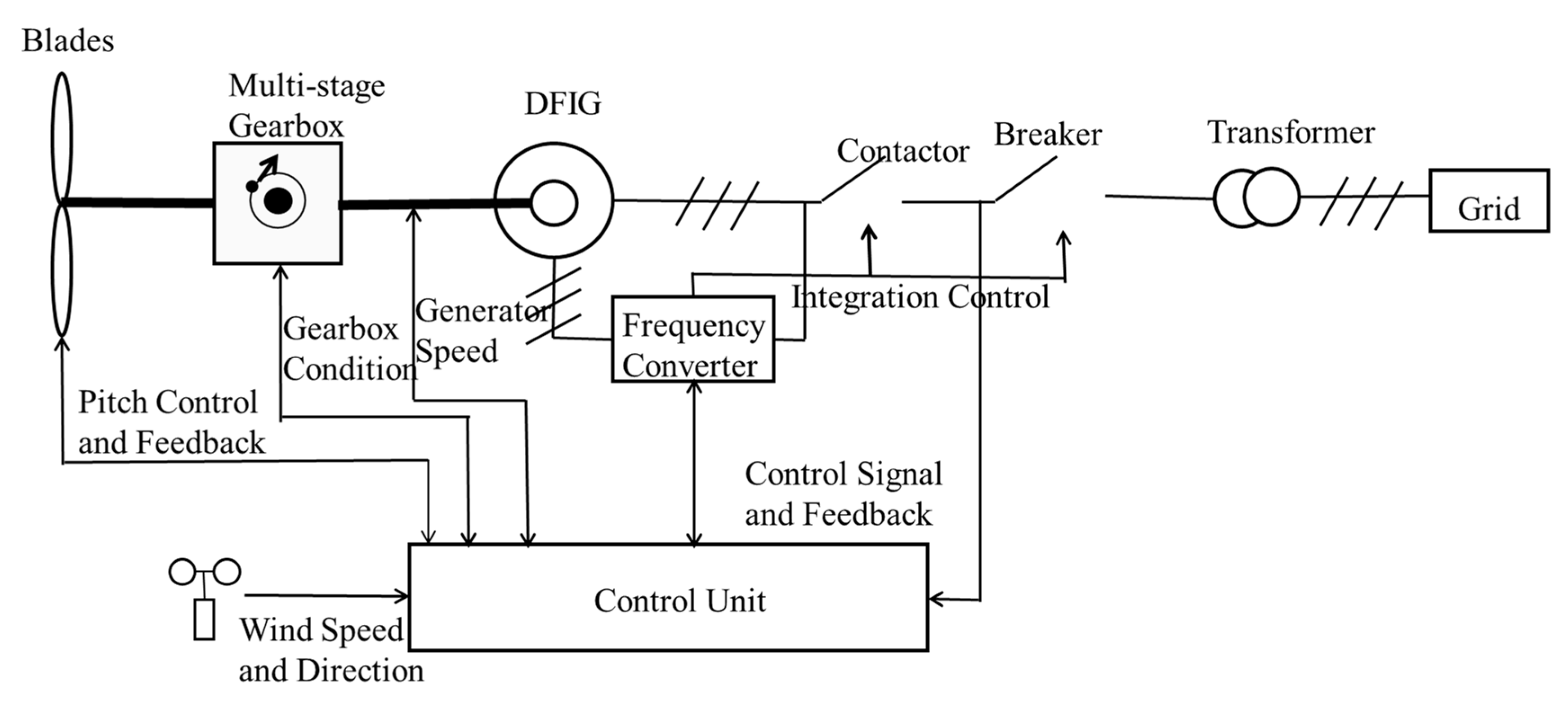
In this section, a one-year SCADA dataset of the WT from a wind farm located in Southern China has been employed for the validation of the proposed methodology. The framework of the studied wind turbine system is shown as
Figure 4, which consists of blades, a multi-stage gearbox, a DFIG, and a frequency converter and control unit. The gearbox is driven by blades to spin the generator to electricity production. The stator of the DFIG converts the mechanical energy with high-speed rotation into power output via the gearbox. Wind turbine faults are found mostly from key elements such as the gearbox, blades, and the generator. These faults are usually associated with high maintenance costs and long downtime of turbine systems. Therefore, troubleshooting and efficient fault identification of gearboxes are of great significance to reduce the lifecycle expenditures on wind turbines, as well as to increase productivities of wind farms.
4.1. Structure of the Wind Turbine Gearbox and the SCADA System
Large-scale wind turbine systems are developed for wind energy harvesting in remote regions, where strong winds are available. The turbine nacelle is sitting on top of a tower which is usually more than 80meters (m) in height.
Figure 4 illustrates the major components of a typical utility-scale wind turbine drivetrain, which is composed of main bearing, main shaft, gearbox, brake, generator shaft, and generator. The generator converts the mechanical energy with high speed to power energy. The blades and rotor hub are supported by main bearings.
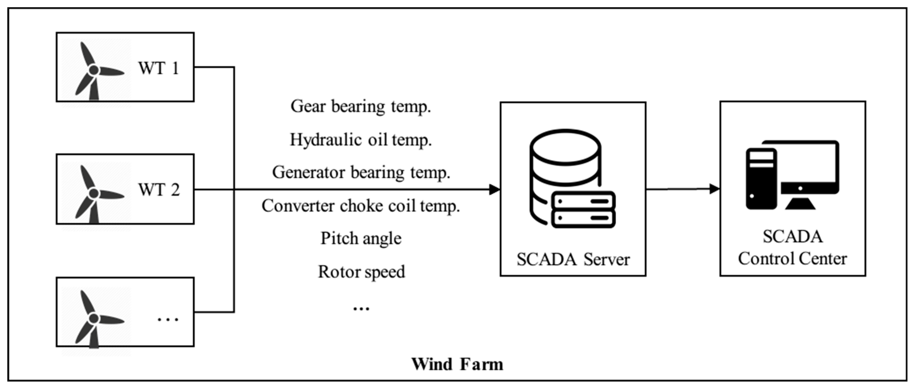
The SCADA system at the wind farm records all wind turbine parameters with a frequency of two seconds. As shown in
Figure 5, each record includes a timestamp, output power, stator current and voltage, wind speed, environmental and nacelle temperatures, as well as the generator stator winding and cooling air temperatures [
18]. Indeed, there are 34 variables in total including internal parameters such as bearing and lubricant temperatures, as well as external parameters like environmental temperature obtained from the SCADA systems installed at the wind farm. In which the lubricant temperature will be sampled with a resolution of two seconds. These data will be preprocessed through data normalization before analysis. At the same time, the SCADA system keeps a recording of turbine operating and fault information such as startup, shutdown, generator over temperature and pitch system fault. Each fault record is composed of a timestamp, a state number, and the fault information.
4.2. Data Preprocessing
To reduce the calculation errors contributed by the numerical differences result from diverse wind turbine systems and to maintain the consistency of the original data structure, the SCADA data is normalized within an interval of [0, 1]. The normal area value is 3 m/s–25 m/s, and the rated wind speed is 12 m/s. The cut-in wind speed is 3 m/s and cut-out wind speed at 25 m/s. As can be seen from
Table 1.
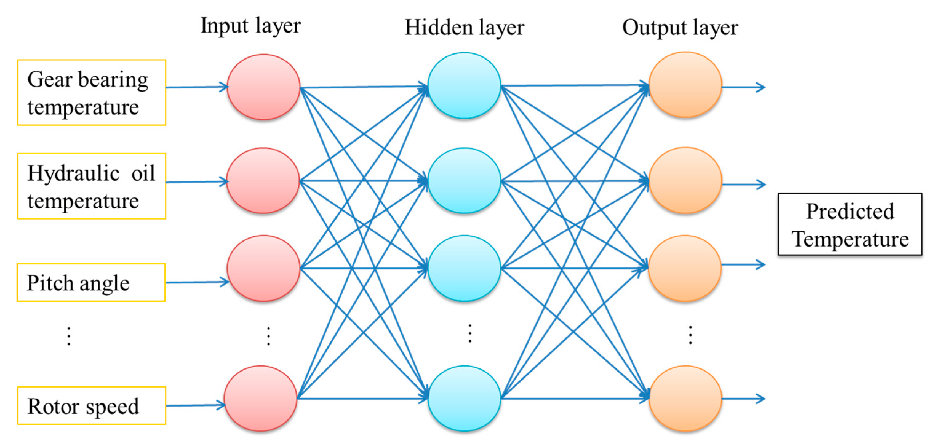
Firstly, the mechanism of wind turbines is analyzed; after that, by combining with expert experience, the comprehensive characteristics of collected data are obtained; and finally, 34 variables are set to support the fault detecting and predicting. Backpropagation neural network (BPNN) including three types of layers: the input layer, the hidden layers, and the output layer. The hidden layers is established to fit the characteristics of our sample data and prevent the over fit. We proposed L2 regularization function in the BPNN.
The architecture of the three-layer BPNN is shown in
Figure 6. The circles in
Figure 6 denotes the neurons of different layers. In this article, we adopted sigmoid function as activation function:
From the wind turbine SCADA datasets, the 34 systematic features listed in
Table 1 can be obtained. To explore the interactions among SCADA parameters, all the monitored data should be normalized. In addition, data normalization can speed up the coverage of the gradient descent algorithm which then leads to the performance enhancement in the machine learning process. In this study, features were calibrated with a linear function, which ensures the values of each feature in data unit-variance. We use the normalization to avoid overweight that certain features of different dimensions may cause. The calibration can be expressed as
where
is the lower bound;
is the upper bound, and
is the normalized value. Please note that the parameters
and
can only be computed within the training data, which would be used in training, validation and testing in the following stages.
4.3. Results and Discussions
With the establishment of the temperature detection model and the processing of all the monitoring data, the WT gearbox working conditions can then be analyzed.
(1) Normal Operation Conditions of Gearboxes
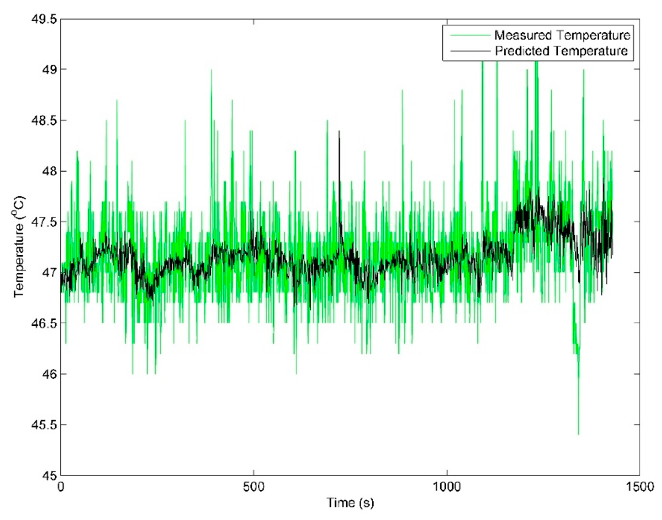
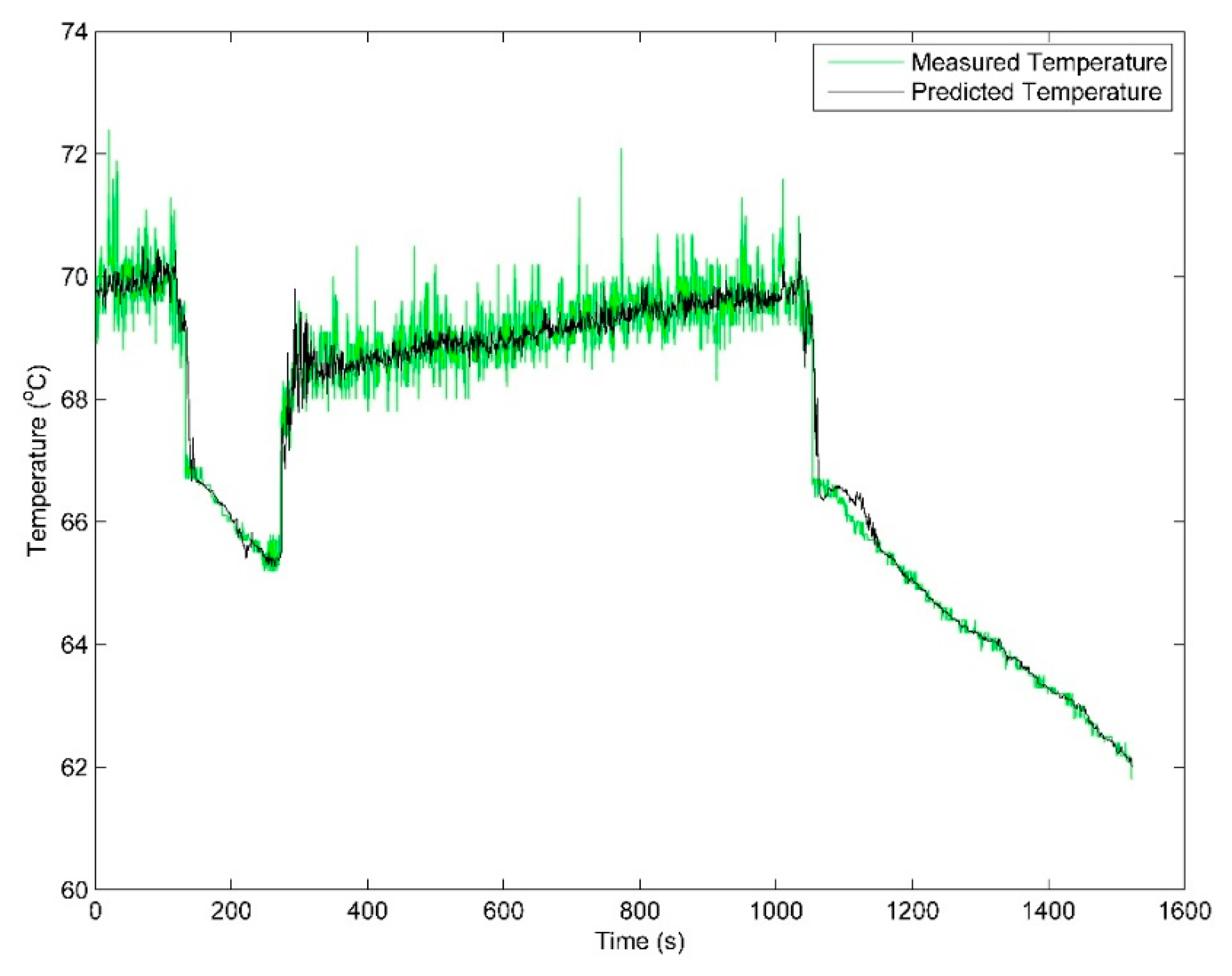
Figure 7 shows the predicted and actual operating temperatures of the gearbox lubricant and bearing. Although there are numerical differences between the measured and estimated values, they present consistency in value changes, or it can be concluded that they are of the same tendency in value variations.
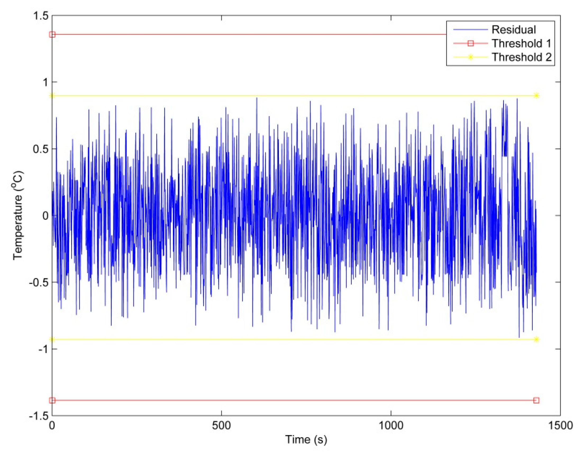
Figure 8 is further employed to find errors in the values of residuals. The diagram indicated that the results detected by the SVM model are desirable when the gearbox is working in normal conditions. With the intervals [
] and [
] are established as warning limit and alarming limit respectively (shown as threshold 1 and threshold 2 respectively in
Figure 8, most values fall in within the thresholds, which indicates that the gearbox was working in normal conditions. In this study, mean absolute percentage error (MAPE), root-mean-square error (RMSE), mean absolute error (MAE), mean absolute percentage error (MAPE) are employed to measure the accuracy of the model. RMSE is an estimator that can measure the deviation between the observed value and the real value. While the mean absolute MAE is a measure of the difference between two continuous variables that can be used to reflect the accuracy of the model. MAPE considering both the error between the true value and the predicted value, and the ratio between the error and the true value, thus, it supports a good evaluation of the stability of the model. In
Figure 7, the MAPE, RMSE, MAE are 0.4572, 0.3500, and 0.0074, respectively.
(2) Abnormal Operating Conditions of Gearboxes
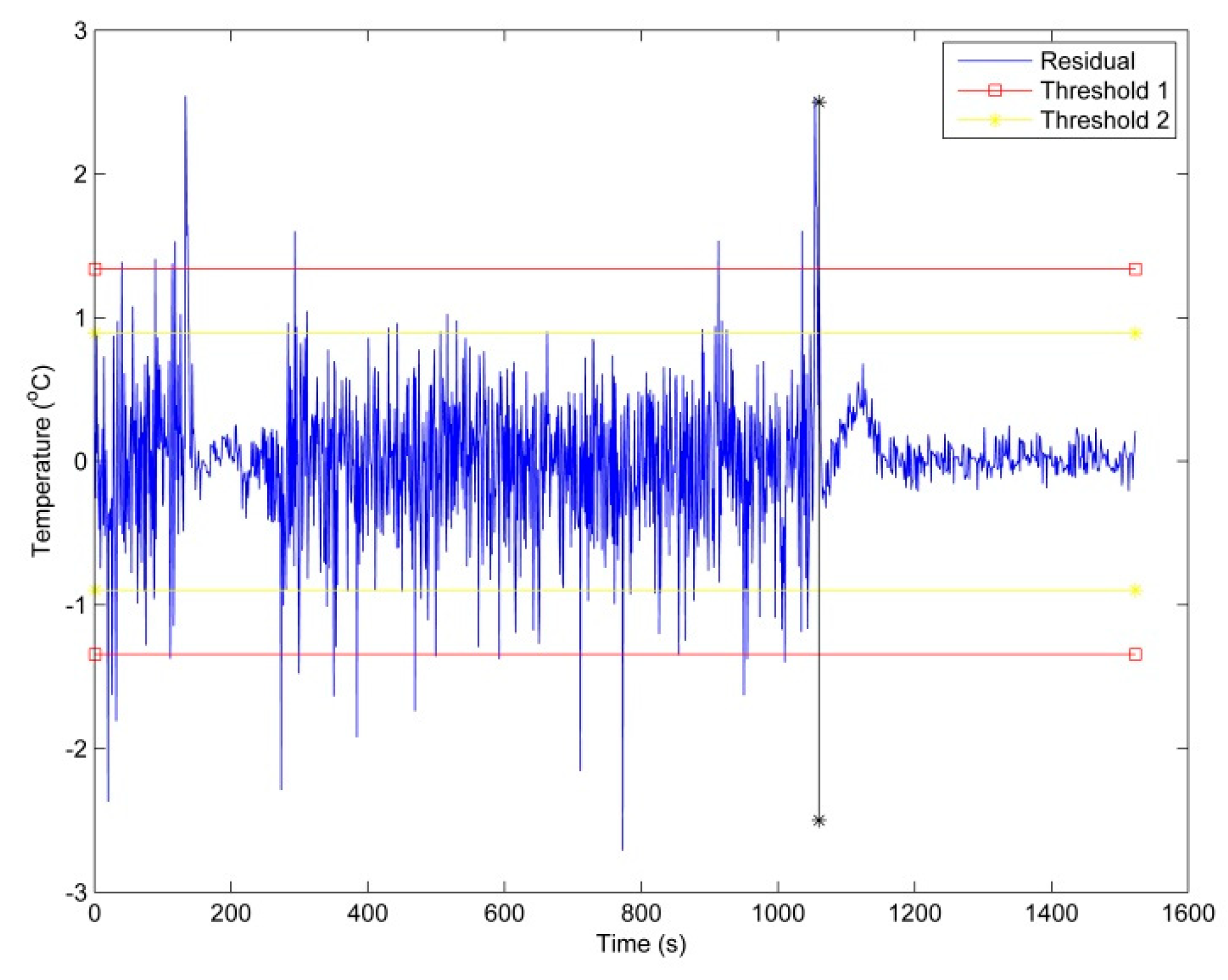
Figure 9 illustrates a detection analysis of an abnormal gearbox installed at the 5# wind turbine on July 10th. As shown in the diagram, the MAPE, RMSE, MAE is 0.4572, 0.3500, and 0.0074, respectively. While the oil temperatures of the gearbox predicted with the SVM model demonstrates a close matching with the monitoring values. That is further supported by the diagram shown in
Figure 10. It then can be concluded that the residual between predicting and monitoring values is growing. As a result, the residual has gradually deviated from the thresholds. This trend also indicates that there is an unbalanced load resulting in friction between the main shaft and the bearing.
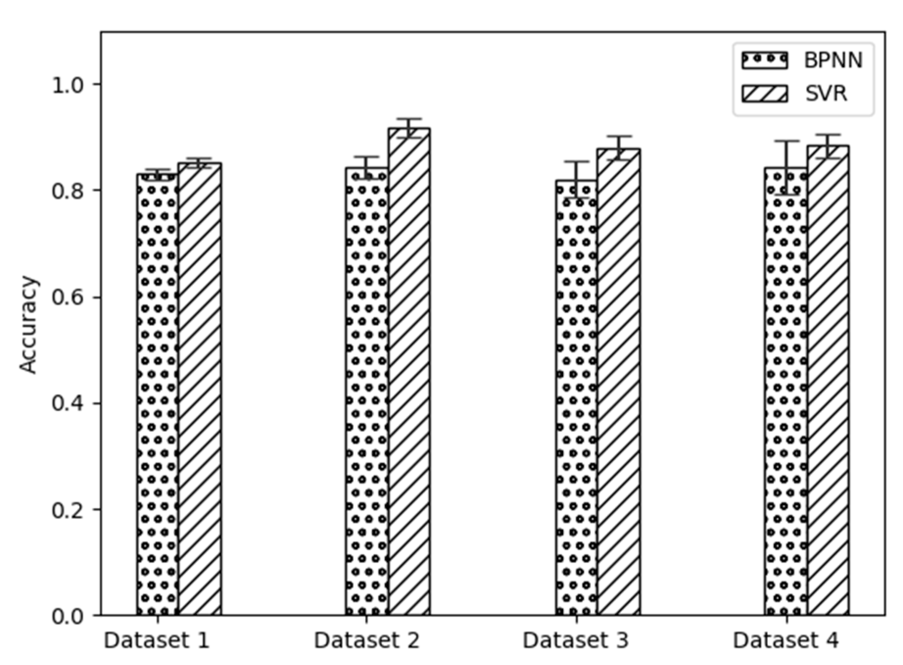
Back Propagation Neural Network (BPNN) is a basic neural network widely used in fault diagnosis, which is generally built as a feed-forward multi-layer network according to the error backpropagation algorithm. To further validate the proposed methodology, a comparative study was also conducted between the methods developed in this research with a BPNN. The results are shown in
Table 2 and
Figure 11. As shown in
Table 2, the average troubleshooting rates achieved by SVR are 0.97%, 7.47%, 3.24%, and 24.26% higher than BPNN in dataset 1 to dataset 4 respectively. While
Figure 11 presents the mean and Standard Deviation of the BPNN and SVR fault detection accurracy. It then can be concluded that SVR shows lower variability than BPNN in the experiments conducted.
5. Concluding Remarks
This study presents an SVR based method which is of the ability in troubleshooting for large-scale wind turbines. An SVR model has been developed for the implementation of fault diagnosis and forecasting with the monitoring data collected from a SCADA system involved for analysis. A case study was carried out to validate the proposed methodology, and the results indicated that the SVR model can forecast faults effectively. In addition, a comparative study was employed to validate the efficacy of the proposed method. And the results indicated that the SVR based method developed in this research is of better performance in troubleshooting compared with a BPNN. Experiments also demonstrated that the SVR model can provide a feasible solution for the real-time online detection of wind turbine faults.
In light of the above findings, suggestions for future studies might be focused on the following fields: (1) preprocessing of the wind turbine fault diagnosis data and the selecting of fault features, which are the foundations of SVR-based troubleshooting operations. (2) Studies of the imbalance problems in wind turbine troubleshooting categories, where the amount of normal class samples is of predominate importance while the size of fault class samples is of unneglectable effects. However, it is often difficult to obtain desirable troubleshooting with single-disciplinary machine learning algorithms.


