Aerodynamics of Monolithic Matrices for Supporting Solid Reactant or Catalyst

Institute of Thermomechanics, Czech Academy of Sciences, v.v.i., 182 00 Praha 8, Czech Republic
Energies 2019, 12(17), 3398; https://doi.org/10.3390/en12173398
Submission received: 24 June 2019
/
Revised: 15 July 2019
/
Accepted: 16 July 2019
/
Published: 3 September 2019
(This article belongs to the Special Issue Fluid Mechanics and Thermodynamics: Theory, Methods and Applications)
Abstract
:Heterogeneous solid/fluid chemical reactions—as well as reactions dependent on solid catalysts—require spreading the active solid substance on the largest accessible area. The solution is a thin layer covering as much as possible convoluted surface of an inert support. This is nowadays the internal surface of narrow parallel passages. The supporting body is usually ceramic, its passages now mostly of square cross section. Reliable detailed knowledge of pressure drop across the set of passages has to be available, especially for flow control based on fluid property changes (e.g., with temperature or fluid composition). This paper presents results of laboratory measurements as well as numerical flowfield computations of the passage flows, with discovered universal law.
1. Introduction
Heterogeneous gas/solid or liquid/solid chemical reactions are more often carried out and are of higher importance than might appear at first sight. Typical examples are the oxidation of the solid, oxides reduction, sublimation into gas flow, dissolution in liquid, and chemical vapour deposition. Of really high importance are reactions in which the activation energy is decreased by solid catalysts. These reactions depend very much upon the size of the available solid surface and ease of access to it. Recognition of the catalytic effect—and coining the name for it—was by Berselius in 1835. Soon thereafter followed uses in industrial chemistry and then, at the beginning of 19th century, became indispensable typically iron-based catalysts for the large-scale production of nitrogen-based explosives. Mutually contradictory requirements, of large surfaces of the catalysts or reactant and a small reactor size were solved by spreading the solid in a thin layer over a chemically neutral support. While the reactant layer has to be regenerated, that of catalyst is practically invariant so that in this latter case may suffice a layer of only sub-micrometer thickness—a welcome fact in view of the expensive nature of many catalysts (often precious metals: platinum, palladium, and rhodium). The support on which the active layer is deposited used to be initially in the form of small ceramic pellets, filling in a haphazard manner the reactor inner space. This is now almost universally replaced by the internal surface of many parallel narrow straight passages. The small thickness and large total surface area are often further extended by providing on the surface of the support a porous layer of 20–30 μm thin washcoat.
2. Crucial Role of Car Exhaust Aftertreatment
Really large-scale use of the heterogeneous catalytic reactions came with the requirements demanded on automobile engine exhaust emission control. For this purpose, the reactors are manufactured worldwide at a rate of thousands per day—adding to those millions already in use. The idea of suppressing the car engine emissions using catalysis was originated by Houdry, an engineer who acquired experience with catalysis in petrochemical industry. He patented the idea of use in car exhaust already before fifties of the last century [1,2]—at a time when it did not find acceptance because suitable catalysts would be poisoned by tetraethyl lead, then universally used anti-knock additive. A change in attitude was caused by the request of the US Environmental Protection Agency in 1970. It enforced mandatory car engine emission limits to begin from 1975. The request initially seemed to endanger the very idea of combustion engines as we know them meaning loss of all the huge sums of money previously invested in their development. The ideas from Reference [1] and other early pioneers were then welcome as a god-sent deliverance — since meeting the regulations could be achieved by mere incorporation of a catalytic reactor into the car exhaust system and the removal of tetraethyl from the fuel.
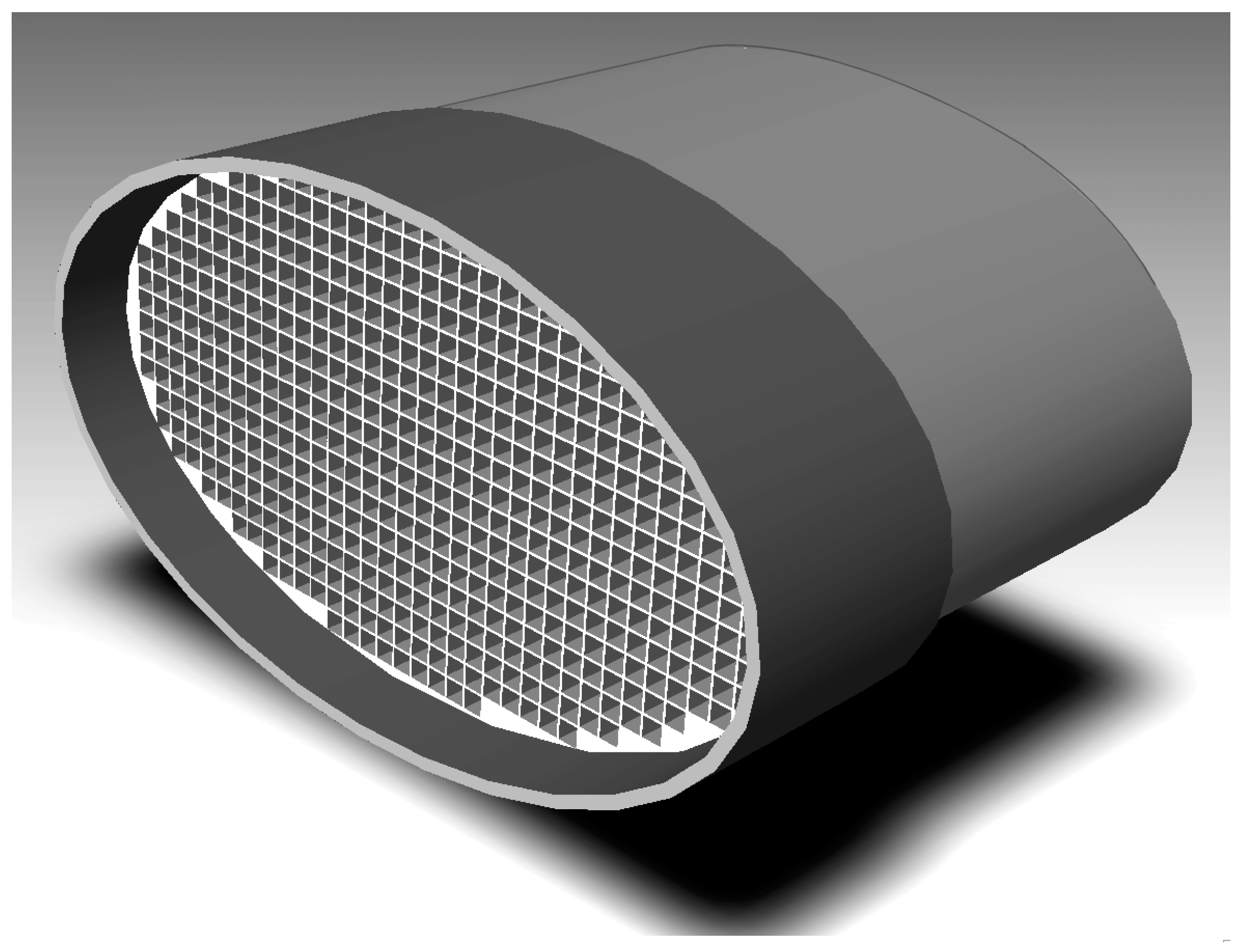
The earliest catalytic reactors for cars were arranged with the classic thin layer spread on inert pellets filling the reactor space. Disadvantages of this approach were recognized quite soon. The first one is the non-negligible proportion of pellets surface in mutual contacts, not accessible for the reactants. Even more important was the second problem: the catalyst layer soon became worn off due to pellet motions caused by vibration of the vehicle. A solution was initially sought in catalyst support made by wounding pre-deformed thin metal sheet strips. Their deformation was shaped to minimise strip contacts and to leave empty space for the flow passages. A typical case is shown, e.g., in Reference [3]. The present-day standard is different: it is a single monolithic ceramic matrix shown in Figure 1, with parallel channels, as foreseen (with different pas-sage geometry) already by Houdry, as seen in Reference [2]. Present-day matrices [4,5,6,7,8] are usually made by extruding a mold of cordierite 2MgO*2Al2O3*5SiO2. After drying and sintering, this material exhibits sufficient mechanical strength and very small thermal expansion. The extrusion die has a large number of fine cores, nowadays it is mostly of a square cross section, see Figure 2 and Figure 3. Each core during the extrusion leaves, in the monolith, Figure 4 and Figure 5, a passage that is now often with its wall thinning at the ends, as shown in Figure 2 and Figure 6 to improve the gas inflow into the passages.
3. Cold Flowfield Inside the Catalytic Reactor
Presence of the catalytic reactor causing increased pressure drop in engine exhaust was initially a nuisance for car and engine designers, but this was soon found to be less important (the drop may be reduced by making larger the overall face area F of the matrix, Figure 3 and Figure 4) and the research activities were directed elsewhere—mainly to the problems associated with the rather small temperature “windows” within which a particular catalyst is effective enough and yet not undergoing irreversible changes by overheating. Receiving particular attention in the catalytic reactor research was then the non-uniformity of temperatures in individual parallel passages. Examples are in References [9,10,11,12,13]. The temperature differences are due to the required total matrix face area F being substantially larger than the exhaust pipe cross section that brings the gas to the matrix. This incongruence of areas causes flow separation from the inner walls of reactor body upstream from the matrix entrance. If this effect is left unattended, a gas jet is formed, impinging only upon the small central part of the matrix face. The exothermic character of the combustion reaction in the reactor causes there a significantly higher local temperatures than in the outer parts. A remedy was found in shaping a more regular area transition at the reactor body entrance and also—following the principles of flow bifurcation [14]—by increasing the aerodynamic drag of the passages (making them more narrow and long helps the flow distribution—though it is not welcome from the pressure drop point of view). The development of momentum transport boundary layer in narrow passages is discussed (for the closely related case of circular cross section) in References [15,16].
Later, however, several direction requests for a deeper understanding of the aerodynamics of the flow in the matrix passages came. One of the requests resulted from the growing awareness of fuel economy, needing a better adjustment of reactor aerodynamic properties. Additionally, the optimization of catalysts to obtain wider temperature windows is important, e.g., Reference [17]. There is also a trend to place, into the car exhaust system, several alternative reactors, at different downstream distances from the engine (and hence at different local temperatures of the gas) and with the catalysts there having different temperature windows, the gas flow switched between them. In principle it is sound, but the switching of the flow into particular instantaneous flowpath between the available reactors [18] necessitates having in the exhaust system several valves, which in their traditional configurations, with mechanical moved components, were the weak spots. Exposed to high temperatures and water sprays from wheels in the typical underfloor locations—and to vibration and accelerations—the valves tended to endanger the overall reliability of the car and the desirable goal of its no maintenance. The solution was found in passive fluidic valves without moving components, based on the Coanda effect [19,20]. The flow is switched in response to changes in the aerodynamic load, which the fluidic valve experiences at its exits—as discussed, e.g., in Reference [18]. Fluidic valves are inexpensive, in principle they are nothing more than just a specially shaped gas flow cavities. They are thus just a solid mechanical component, offering no opportunity to failure due to loose or lost screws, broken springs, membranes, or leaky seals of mechanical valves. Their sensitivity to the varied aerodynamic load [17], however, necessitates knowing precisely, at the design stage, the minute quantitative details of the load behavior. When mastered, this idea can be applied to rather complex operations, such as in the regeneration of a reactor when sooth accumulation reaches a certain limit [18] and calls for burning out—or even in the variable configurations of gas flowpath, switching it between alternative reactors so that each may operate at its optimum temperature [13].
4. Pressure Loss Experiments
4.1. Models and Procedures
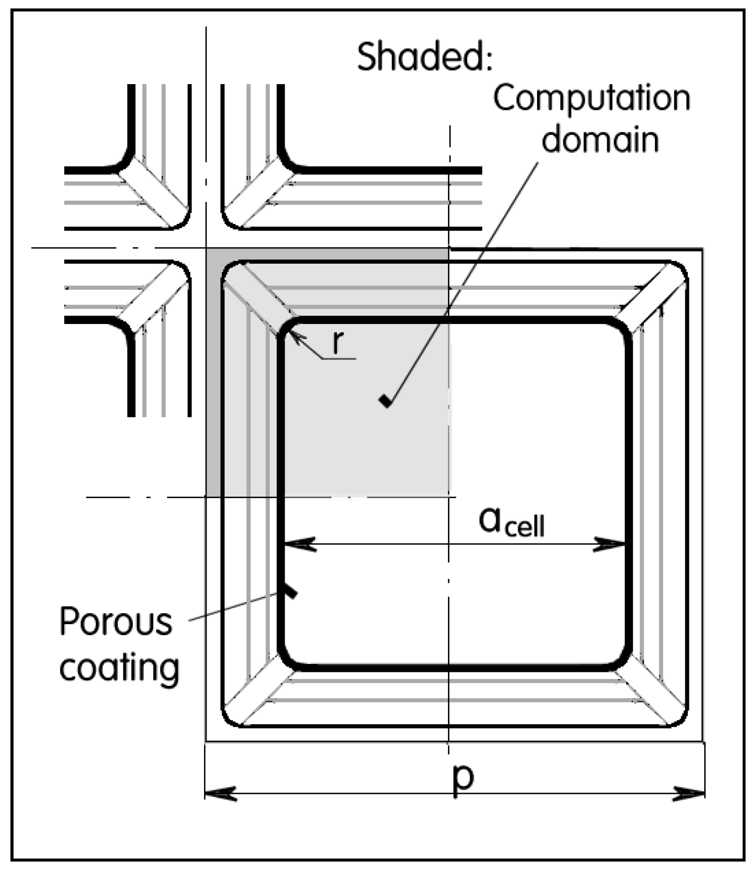
The request for more detailed knowledge called for introducing a research project, beginning with understanding cold air-flow. From the point of aerodynamics, monolithic matrices of the investigated type are clusters of a large number of parallel very narrow passages. Over most of the passage length, its cross section is constant, with parallel, mutually orthogonal walls, and the corners rounded by very small radius r (Figure 2). The flow in this constant-area region is simple. Complications exist at the passage entrance and exit, where the flow has to accept a change in velocity caused by the partial blockage of the flow by the inter-passage walls.
Two matrix samples were available for author’s laboratory investigations of the cold flows, both with the internal surfaces covered by the washcoat.
- (1)
- The sample A was a cylinder-shaped cordierite monolith of diameter d = 135.9 mm, overall length in streamwise direction 152.2 mm, cell width αcell = 0.875 mm, pitch distance between individual cells 1.26 mm, and the width of the walls between cells b = 0.387 mm. The largest number of cells in a single row along the matrix diameter was in the center, where there were 108 square-shaped cells.
- (2)
- The other available B was also shaped as a cylindrical monolith of overall diameter d = 127.1 mm, overall length in streamwise direction 152.0 mm, cell width αcell = 1.0 mm, and pitch between individual cells 1.27 mm, with slightly smaller wall thickness, Figure 5. There were 100 cells with a maximum in the diameter direction. Both ends of the inter-passage walls were had an easier flow transition into and out of the matrix and was made thinner, as shown in Figure 6. At the entrance, the walls were only 0.1 mm thin, gradually increasing to the thickness b = 0.27 mm. Details of the transition geometry in Figure 6 are the averages from a large number of measurements.
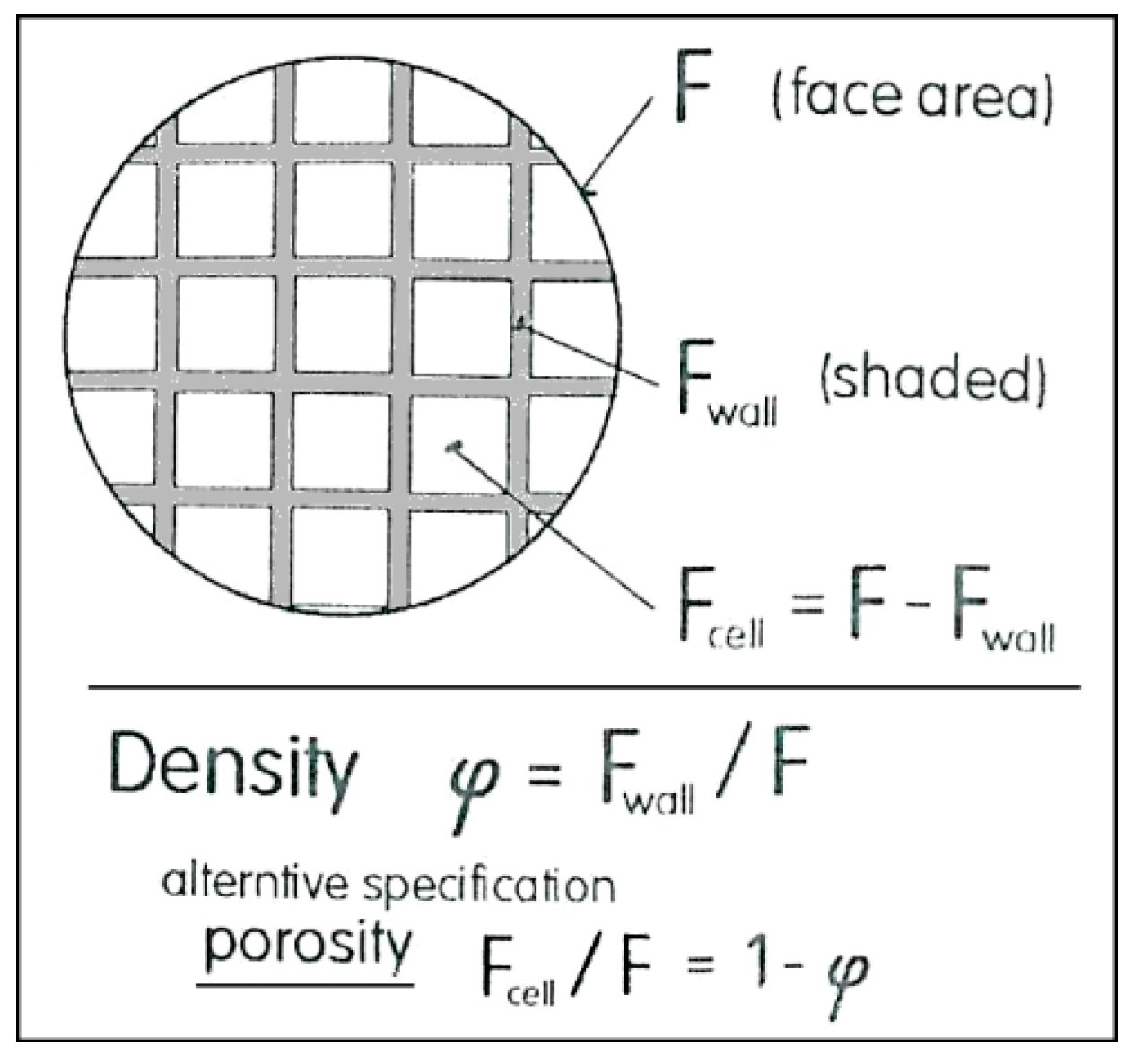
An important factor from the point of view of aerodynamics of objects is similarly the partly blocking of the total area in the area density φ
The ratio of the open area Fcell of the cells in the sample to the round face total area F = π d2/4 (Figure 3 and Figure 4). The density values for the samples A and B were φ = 0. 52 and φ = 0.38, respectively.
The matrix samples were tested in the laboratory by passing a measured air flow at laboratory room temperature though each of them, while the pressure drop across the matrix was measured. The total mass flow rate [kg/s] of air was measured by a flowme ter. Nominal values of the flow velocity (i.e., neglecting the complexities of the actual velocity profiles) [m/s] was evaluated from the measured flow rate as
where [m3/kg] is the specific volume of the air. In the tests, this nominal velocity inside the matrix cells varied in the range from approximately ~0.5 m/s to ~4.5 m/s.
As the air flows in the tests were steady, the pressure drop [Pa] across the passages could be measured by simple liquid-filled U-tube manometers. Measured data values are plotted in Figure 7. It is evident, as expected, that the pressure drop across the matrix A of higher area density is higher at the same flow velocity .
4.2. Data Processing and Discovered Universal Law
As is usual in aerodynamics, the experimental data values on both co-ordinates in Figure 7 were here also converted into dimensionless variables. The velocity on the horizontal co-ordinate was converted into
this is Reynolds number of the flow in the cell (passage) of width acell. The quantity in the denominator of Equation (3) is the kinematic viscosity of air. Its value during the measurements remained practically constant.
The measured pressure drop values and the corresponding differences in pressure energy were related to the nominal specific kinetic energy of the fluid flow. Again, the specific volume of air in the tests was constant. The result is the Euler number
Both dimensionless quantities defined in Equations (3) and (4) were plotted in logarithmic co-ordinates in Figure 8. The results are remarkable. Straight lines fitted to the data points for both samples were identical. This universality is an important fact that does not seem to be, so farm mentioned in the literature.
The universal power-law line fitted to all collected data is
The reason for this universality is seen in the dominant influence of the passage length. In both cases, the overall length of the two monolith matrix samples A and B were the same at ~152 mm. Explaining this influence of the length l, however, is by no means simple since the two cases differed quite significantly in the relative length λ of the constant-section part of the passage.
5. Numerical Computations
5.1. Used Software
It would be interesting to investigate by computations the invariance of the universality Equation (5). For this purpose, additional tests performed with matrix samples of different lengths should be very useful. Somewhat surprisingly, the author was not able to obtain samples of different lengths from the matrix manufacturers. A way to solve this dilemma was to perform numerical flowfield solutions. With the numerical model there should be, in principle, no limitation to the use of different lengths.
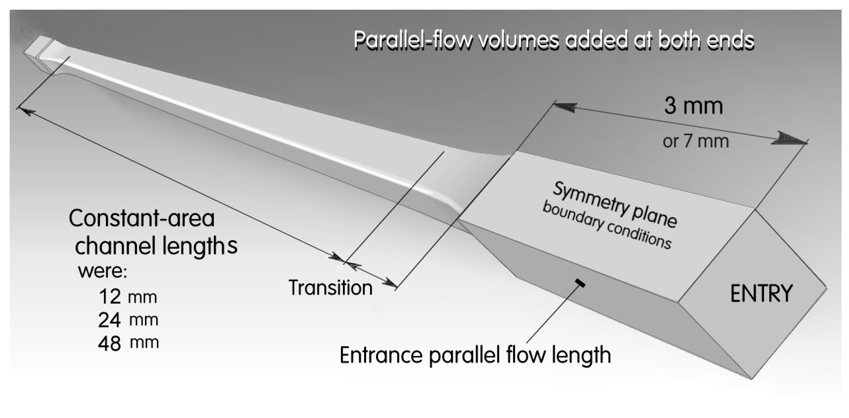
The computations were performed with commercially available finite-difference software FLUENT 15.0, with the initial tetrahedral unstructured mesh set up by software Gambit 2.4.6. Due top the unstructured character, it was possible to gradually refine the mesh in the course of the solutions in the locations with velocity gradient magnitude larger than a chosen limit. This was done by dividing the mesh cells into parts. Velocity gradient limit was gradually decreased in repeated solutions. To simplify the definition of boundary conditions, entrance and exit volumes were added on both ends of the computation domain. In the upstream volume, the inlet velocity was inserted as constant over the entrance plane. On the exit site, the boundary condition was a constant pressure in the whole exit plane. Initially, the streamwise length of the added volume was 7 mm (Figure 9), but later encountered problems with the number of finite volume elements (extent of available computer memory and the solution running time) forced a reduction to only 3 mm. The initial attempts at a solution very soon encountered two non-trivial questions.
5.2. Incongruence of Transversal and Longitudinal Scales
It was acceptable to rely upon the geometric symmetry apparent in the cross-section of the passages seen in Figure 2. This decreased the convergence times of solutions by reducing the number of mesh cells to one quarter of what would be necessary if the computations were run over the full volume of the cell. In spite of the fully three-dimensional computation algorithm, of course, this assumption of symmetry eliminated any (hardly present) swirl in the computed results.
It was, however, decided to stick to three-dimensional reality by not neglecting the existence of the small-radius rounding r = 0.05 mm in the outer corner of the domain. For the effect of this rounding to be felt at all, the circumferential distance between the mesh points on the rounding surface were as small as 0.01 mm. To keep the mesh elements not too elongated (elongation introduces computation errors), the streamwise distance between the mesh points were also to be of the same order of magnitude. For the 152 mm axial length of the channel inside the matrix, this alone would mean the streamwise 15,200 points in which the quantities were to be computed. If there were only 100 data points at each cross section of the domain (which is a small number since it is necessary to have fine mesh at the two side walls of the domain), the number of the data points should be 1.5 million. With such numbers, the computations reaching a reasonable solution convergence lasted agonizingly long. The decision leading to the obtaining of a number of computational results at different flow velocities was to make introductory computation with many shorted passage lengths; at first the length of the constant-cross-section part of the passage was 12 mm. Later, having established the reliability of the data, the computations could be extended to lengths 24 mm, and finally, also again as twice as much at 48 mm. The idea was to use the results for gradually increased lengths as a basis for extrapolations to any channel length.
5.3. Turbulence Model Modified for Low Re
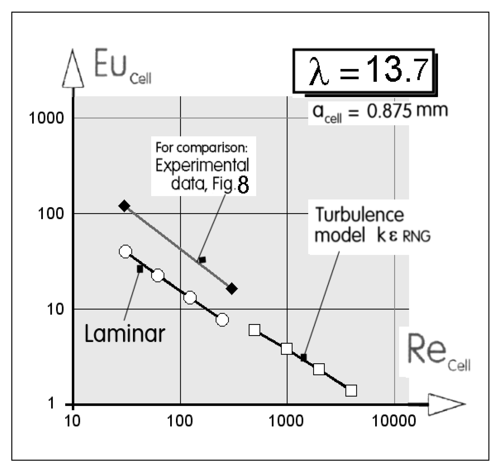
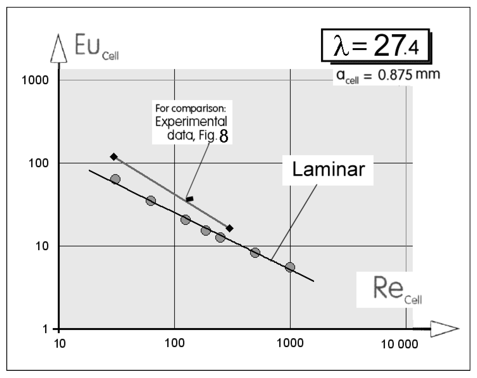
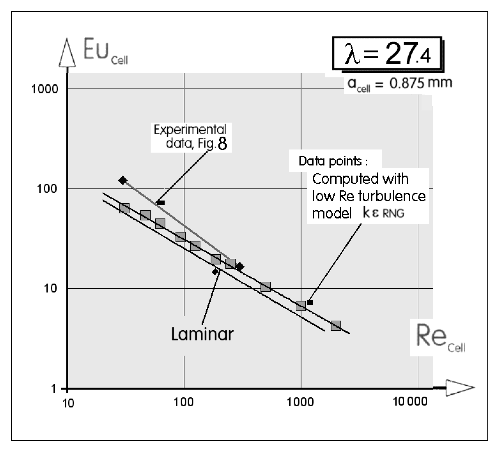
It is obvious from the data values presented in Figure 8 that the cell-size Reynolds numbers in the laboratory measurements were quite low, below ReCell = 300. These are values at which it might be reasonably expected that the flow is of laminar character. The easily varied values of boundary conditions in the computation provided, however, an opportunity to investigate the flow at gradually increased Re and see what happens if the behavior is influenced by turbulence. At any rate, the Reynolds numbers of turbulence at these conditions are, however, quite low. This request modifies the turbulence model. In the previous author’s numerical computations of small-size objects and comparisons with experimental data was found the renormalization group modification satisfaction and is available in the FLUENT package. It was decided to also apply this RNG approach in the present case. The basic turbulence model that was modified was the k–ε two-equation model with standard wall functions. Values of the model constants used in the computations were standard, as delivered by the software supplier. As seen, e.g., in Figure 12, where the computation results are compared with the experimental data from Figure 8, the solutions with the modified turbulence model were extended to the ReCell values as high as ~5000 without any change in the pressure drop character. At lower ReCell values, the computation was also performed—with the same mesh and same other conditions—concurrently with the assumed laminar flow. The computation results presented in Figure 12 were obtained with much shorter passage (for the reasons discussed above in Section 5.2) and hence lower pressure drop. This explains the vertical differences seen between the EuCell values obtained in the experiment and numerical computations. The same comparison is in Figure 13 for the 24 mm long passage of laminar flow computations. Additionally, this passage was much shorter than the one used in the experiment. Of course, the computed EuCell values are therefore lower. Nevertheless, the general character of both approaches may be described as being in agreement. Another comparison diagram of this sort is presented in Figure 14. The data points there were obtained with the modified turbulence model. The only somewhat disappointing aspect of the discussed computation is the behavior of the RNG modification. Ideally, at gradually decreased Re, the results obtained with the modified turbulence model should show a smooth asymptotic approach to the laminar flow results. Diagrams presented in Figures 12–14 do not show such a transition.
5.4. Computation Results
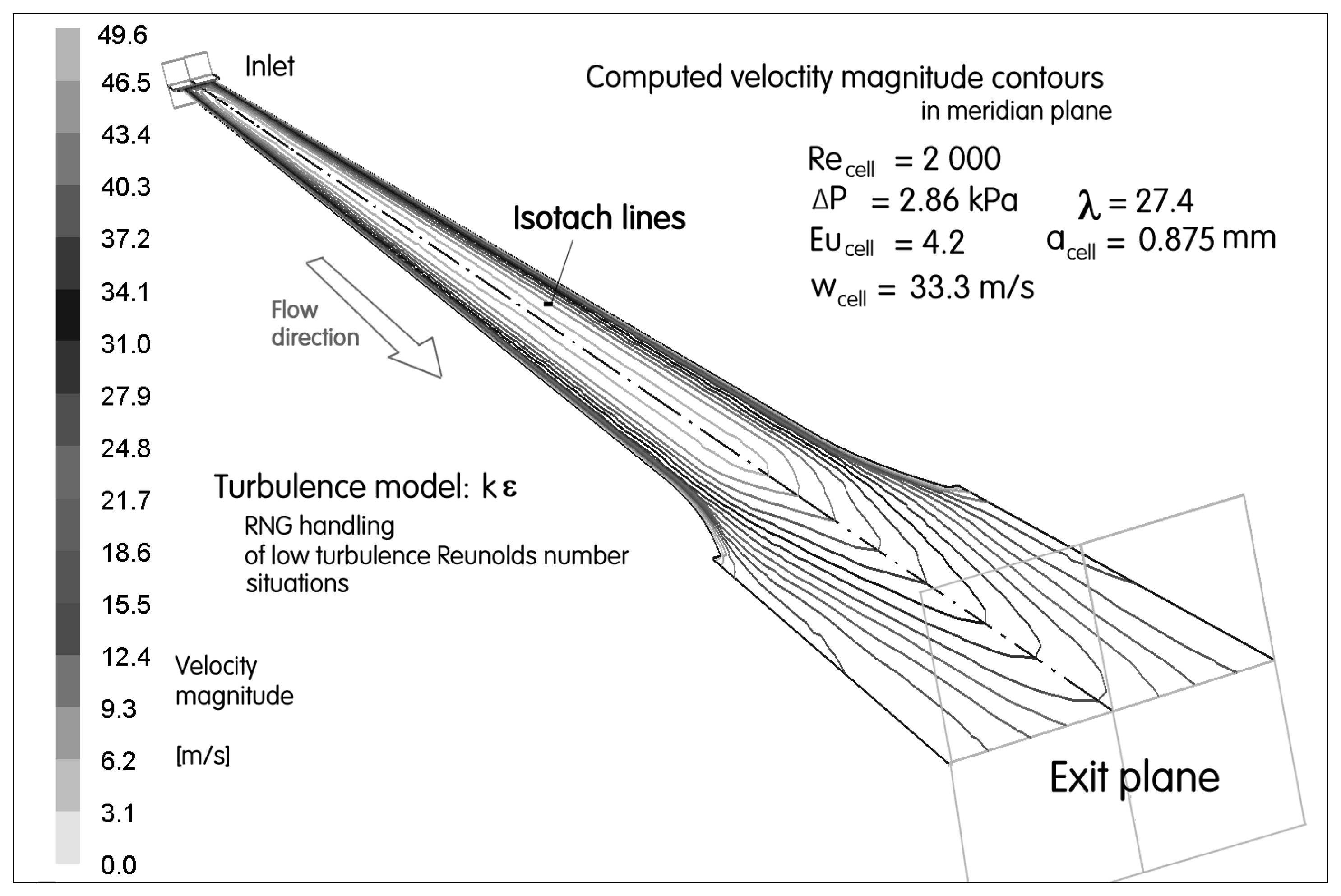
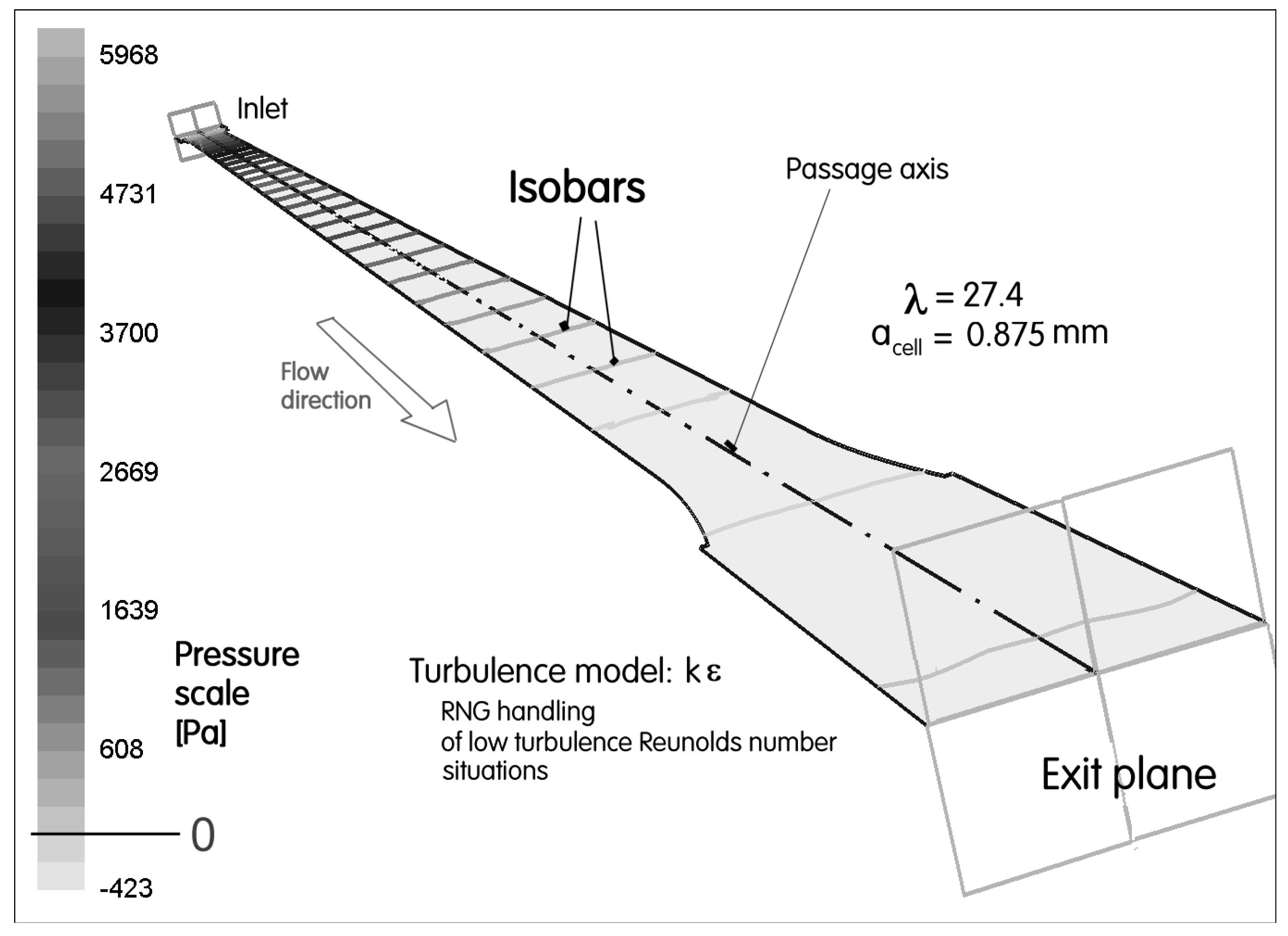
Computed isotachs—lines connected to the locations with the same values of absolute velocity—are presented for passage symmetry plane in Figure 10. The Reynolds number value ReCell = 2000, at which these computations were run, was quite high. This may perhaps be the reason why these isotachs show a distinct boundary layer effect—the velocity gradient concentrating to the vicinity of the passage walls. In the same conditions as in Figure 10 the diagram in following Figure 11 presents computed isobars—the contours of constant pressure on the symmetry plane of the passage. These isobar contours are extremely simple, exhibiting a constant value over the whole cross-section planes. While the used perspective view perhaps does not show it really clearly, an important fact is that the isobars are mutually equidistant—which means the streamwise pressure gradient is constant.
The data in the following figures, Figure 12, Figure 13 and Figure 14, are already mentioned above. As the manageable lengths of computation domain are much shorter than the lengths in the experiment, the expected fact that the computed pressure drops P are lower and also lower are therefore the Euler number values EuCell seen and are plotted on the vertical co-ordinates. The laminar and modeled-turbulence data results on all three diagrams, Figure 12, Figure 13 and Figure 14, are near to each other. The compared Figure 12 and Figure 13 show that, with the longer computation domains in Figure 13, the Euler numbers are higher and nearer to the experimental data (presented by the lowest and largest experiment data points). In the last picture of this series, Figure 14, the line fitted to the experimental results and the line obtained with the laminar model from Figure 13 are compared with laminar regime computation results. As mentioned above in Section 5.3 there is not the expected smooth transition between laminar and modified turbulence regimes. The lines fitted to both are nearly parallel.
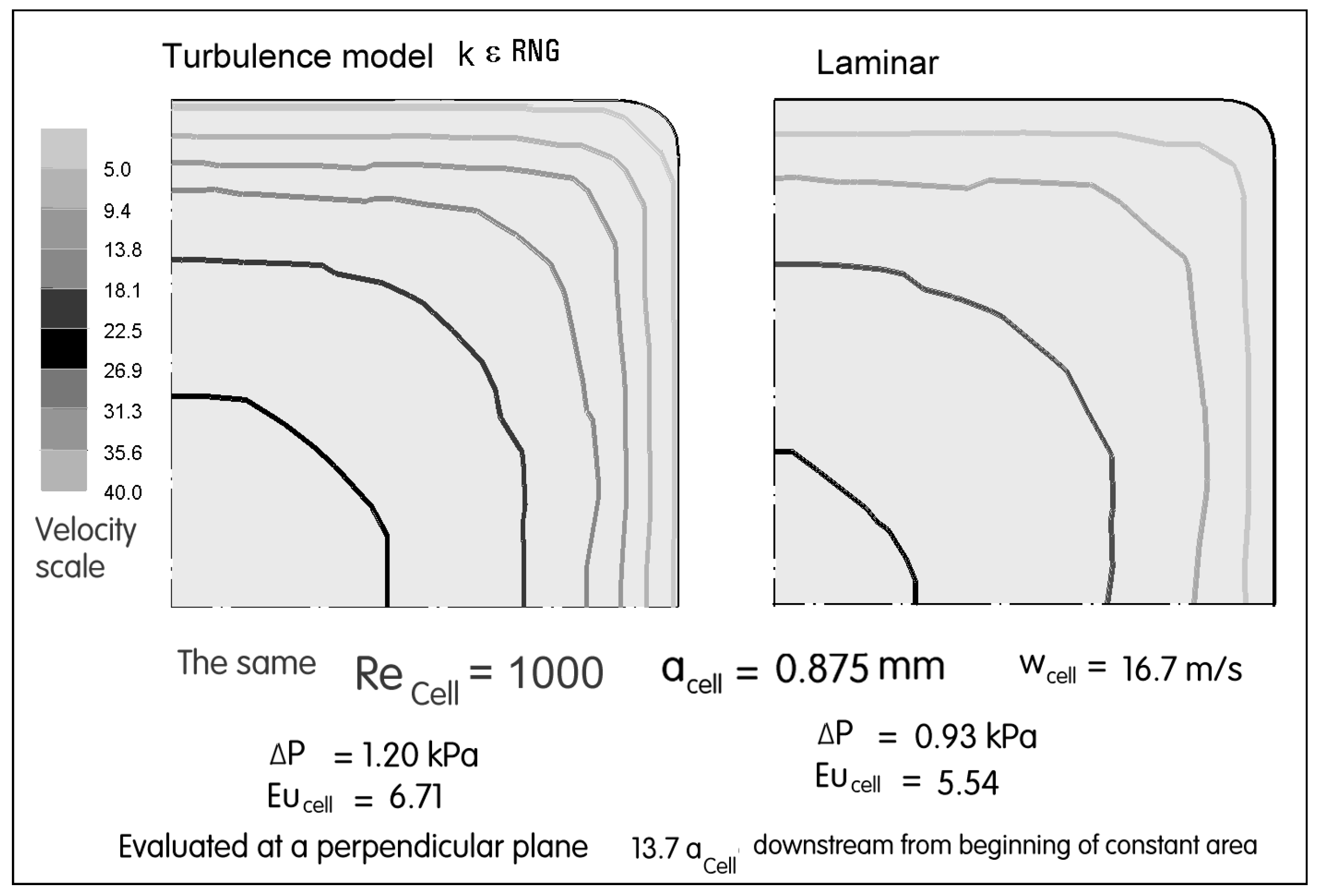
Despite the near EuCell data for the two computation regimes, the character of flow is rather different (considering the relative simplicity of the domain geometry). This is demonstrated for the identical conditions (the only change between the two cases being the different flow model) on the isotachs in transverse cross sections, presented in Figure 15.
The most important results obtained in the computations are the pressure distributions along the passage axis. The heavy line in Figure 12 presents a typical example, with the characteristic constant pressure gradient in the region of the constant shape and size of the passage. In Figure 13, superposed pressure distributions obtained at the same Re are shown. For the purposes of designing monolithic matrices, the axial gradient may be considered constant. There are, in fact, as shown in the presentation Figure 14, slight differences between the slopes dP/dX1, but they may be attributed to the solution conditions (such as, e.g., the number of discretization elements) that could not be exactly the same.
The universality (or, at least, near-universality) presented in Figure 8 is the most important fact that was obtained in this study. It shows that it is quite safe to predict matrix behavior for any passage lengths by extrapolating from these data.
6. Conclusions
For the initial simplification, both experimental investigations and numerical flowfield solutions of the matrix aerodynamics are here limited to cold air-flows. Even within this limit, there are several interesting and practically useful results. One qualitative result is the demonstrated crucial importance of the matrix passage (cell) lengths. Among the quantitative results, the main one is the discovered universal law of the dependence of the pressure drop on the flow rate. This is demonstrated, by the experimental evidence in Figure 8, with the same behavior of the matrices of the same streamwise lengths. Computational results, exhibiting practical universality of the streamwise pressure gradient in Figure 8, make the extrapolations of the results to any length justifiable. This may be of paramount importance for the design of chemical reactors for heterogeneous (fluid/solid) reactions and solid catalysts.
Funding
Author’s investigations were supported by research grant no.17-08218S obtained from GAČR—the Czech Science Foundation. Also received was institutional support RVO: 61388998.
Conflicts of Interest
The author declares that there are no conflict of interest regarding the publication of this paper.
References
- Houdry, E.J. Catalytic Structure and Composition. U.S. Patent 2,742,437, 24 May 1949. [Google Scholar]
- Hougry, E.J. Catalytic Apparatus for Exhaust Gases. U.S. Patent 2,674,521, 5 May 1950. [Google Scholar]
- Baba, N.; Ohsawa, K.; Sugiura, S. Analysis of transient thermal characteristics of automobile catalyst converters. Trans. Jpn. Soc. Mech. Eng. 1996, 17, 273–279. [Google Scholar]
- Benbow, J.; Lord, L. Catalyst Support. U.S. Patent 3,824,196, 7 May 1971. [Google Scholar]
- Berdys, M.; Koreniuk, A.; Maresz, K.; Pudło, W.; Jarzębski, A.B.; Mrowiec-Białoń, J. Fabrication and performance of monolithic continuous-flow silica miroreactors. Chem. Eng. J. 2015, 282, 137–141. [Google Scholar] [CrossRef]
- Cybulski, A.; Moulijn, J.A. Monoliths in heterogeneous catalysis. Catal. Rev. 1994, 36, 179. [Google Scholar] [CrossRef]
- Somers, A.V.; Berg, M.; Shukle, A.A. Cordierite Refractory Compositions and Method of Forming Same. U.S. Patent 3,954,672, 4 May 1974. [Google Scholar]
- Wilkin, O.M.; Allen, R.W.K.; Maitlis, M.; Tippetts, J.R.; Turner, M.L.; Tesar, V.; Haynes, A.; Pitt, M.J.; Low, Y.Y.; Sowerby, B.; et al. High throughput testing of catalysts. In Principles and Methods for Accelerated Catalyst Design and Testing; Douane, E.G., Ed.; Kluwer: Alphen aan den Rijn, The Netherlands, 2002. [Google Scholar]
- Kim, J.Y.; Lai, M.-C.; Li, P.; Chui, G.K. Flow distribution and pressure drop in diffuser-monolith flows. Trans. ASME J. Fluids Eng. 1995, 117, 362–368. [Google Scholar] [CrossRef]
- Lopes, J.P.; Rodrigues, A.E. Monolith Reactors. In Multiphase Catalytic Reactors: Theory, Design, Manufacturing, and Applications; Önsan, Z.I., Avci, A.K., Eds.; John Wiley & Sons, Inc.: Hoboken, NJ, USA, 2016. [Google Scholar]
- Masood, A. Simulation of Flow Inside a Catalytic Converter. Open Access on Internet, March 2016. [Google Scholar]
- Oh, S.H.; Cavendish, I.C. Transients of monolithic catalytic converters: Response to step changes in feedstream temperature as related to controlling automobile emissions. Ind. Eng. Chem. Prod. Res. Dev. 1982, 21, 29–37. [Google Scholar] [CrossRef]
- Tesař, V. No-moving-part valve for automatic flow switching. Chem. Eng. J. 2010, 162, 278–295. [Google Scholar] [CrossRef]
- Tesař, V. Characterisation of three-terminal fluidic elements and solution of bifurcated-flow circuits using the concept of equivalent dissipance. J. Fluid Control Fluid. Q. 1981, 13, 55–79. [Google Scholar]
- Tesař, V. Recent advances in characterisation of subsonic axisymmetric nozzles. EPJ Web Conf. 2018, 180, 02107. [Google Scholar] [CrossRef]
- Tesař, V. Geometric quasi-similarity: Case of nozzles with quadrant-shaped inlet. Sens. Actuators A Phys. 2016, 248, 246–256. [Google Scholar] [CrossRef]
- Williams, J. Monolithic structures, materials, properties and uses. Catal. Today 2001, 69, 3–9. [Google Scholar] [CrossRef]
- Tesař, V. Fluidic valves for variable-configuration gas treatment. Chem. Eng. Res. Des. 2005, 83, 1111–1121. [Google Scholar] [CrossRef]
- Coanda, H. Device for Deflecting a Stream of Elastic Fluid Projected into an Elastic Fluid. U.S. Patent 2,052,869, September 1936. [Google Scholar]
- Tesař, V. Fluidic control of reactor flow—Pressure drop matching. Chem. Eng. Res. Des. 2009, 87, 817–832. [Google Scholar] [CrossRef]
Figure 1.
Ceramic monolithic matrix in a version resembling those used in car exhaust gas aftertreatment. Modern catalytic reactors for internal combustion engines are generally larger than this example, with very fine channels (around 100–250 parallel passages of millimetre size in the horizontal row). The typical elliptic shape seen here makes easier fitting into the usual underfloor car locations.

Figure 2.
Typical square cross section of the passage in present-day ceramic matrices, seen in the flow direction. The key geometric factor is the cell width acell. The gray quadrant is the domain in which numerical flowfield solution employing the geometric symmetries was performed.
Figure 2.
Typical square cross section of the passage in present-day ceramic matrices, seen in the flow direction. The key geometric factor is the cell width acell. The gray quadrant is the domain in which numerical flowfield solution employing the geometric symmetries was performed.

Figure 3.
Definition of the area density characterizing the availability of free flow area of passages. It is a factor in experimental investigation that was typically performed with parallel flow over a determined face area F of the matrix.
Figure 3.
Definition of the area density characterizing the availability of free flow area of passages. It is a factor in experimental investigation that was typically performed with parallel flow over a determined face area F of the matrix.

Figure 4.
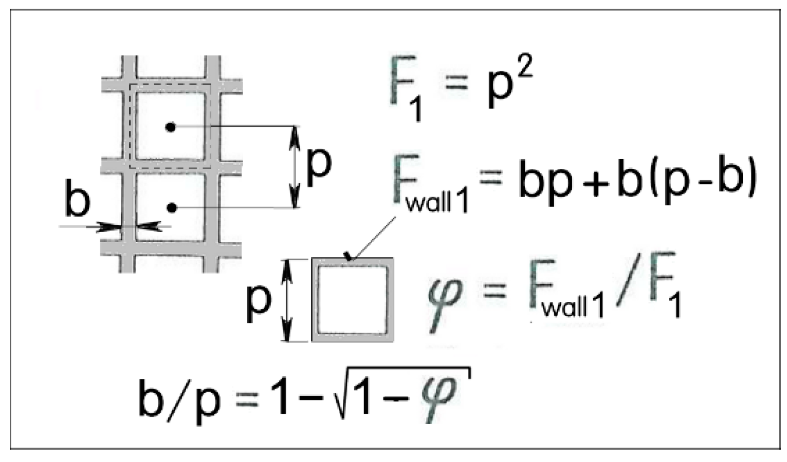
Other important factors (apart from those in Figure 3) used to characterize available flowpath area in a matrix is the cell pitch p and matrix wall thickness b.
Figure 4.
Other important factors (apart from those in Figure 3) used to characterize available flowpath area in a matrix is the cell pitch p and matrix wall thickness b.

Figure 5.
Dependence between the channel area density (defined in Figure 2) and the relative thickness b/p of channel walls. Points A and B represent the matrix samples used in the discussed experiments.
Figure 5.
Dependence between the channel area density (defined in Figure 2) and the relative thickness b/p of channel walls. Points A and B represent the matrix samples used in the discussed experiments.

Figure 6.
Details of the typical gradual reduction of the flow area at the entrance into the matric passage (the axial view is in Figure 2). Indicated dimensions are those of the investigated matrix type A. The same gradual wall thickness variation is at the passage exit.
Figure 6.
Details of the typical gradual reduction of the flow area at the entrance into the matric passage (the axial view is in Figure 2). Indicated dimensions are those of the investigated matrix type A. The same gradual wall thickness variation is at the passage exit.

Figure 7.
Experimental pressure drop data obtained with the two different matrix samples A and B. They are the same as what is nowadays used in standard car emission control.
Figure 7.
Experimental pressure drop data obtained with the two different matrix samples A and B. They are the same as what is nowadays used in standard car emission control.

Figure 8.
Data from Figure 7 non-dimensionalized—plotted as dependence of Euler number on cell Reynolds number. They could be fitted by the single universal power law line.
Figure 8.
Data from Figure 7 non-dimensionalized—plotted as dependence of Euler number on cell Reynolds number. They could be fitted by the single universal power law line.

Figure 9.
Perspective view of the computation domain—one quarter is a single passage (shaded in the end view presented in Figure 2).
Figure 9.
Perspective view of the computation domain—one quarter is a single passage (shaded in the end view presented in Figure 2).

Figure 10.
An example of the results of numerical flowfield computations: Distribution of absolute velocity contours in the meridian plane of the computation domain. Only the contours on the right of the axis was actually computed—the left side is a mirror image.
Figure 10.
An example of the results of numerical flowfield computations: Distribution of absolute velocity contours in the meridian plane of the computation domain. Only the contours on the right of the axis was actually computed—the left side is a mirror image.

Figure 11.
In contrast to the isotachs in Figure 10, the computed contours of pressure in the passage, shown here, are very simply equidistant planes perpendicular to the axis.
Figure 11.
In contrast to the isotachs in Figure 10, the computed contours of pressure in the passage, shown here, are very simply equidistant planes perpendicular to the axis.

Figure 12.
Computed pressure drop results in the co-ordinates from Figure 8, obtained with very short passage lengths.
Figure 12.
Computed pressure drop results in the co-ordinates from Figure 8, obtained with very short passage lengths.

Figure 13.
Pressure drops across a longer computation domain—still very much shorter than the matrix passage length in the experiment, Figure 8—obtained by numerical solutions assuming laminar flow.
Figure 13.
Pressure drops across a longer computation domain—still very much shorter than the matrix passage length in the experiment, Figure 8—obtained by numerical solutions assuming laminar flow.

Figure 14.
Computation results obtained with the turbulence model modified for very low turbulence Reynolds numbers—under the same conditions as Figure 13.
Figure 14.
Computation results obtained with the turbulence model modified for very low turbulence Reynolds numbers—under the same conditions as Figure 13.

Figure 15.
Comparison of computed isotach lines in the section across constant-area part of the passage obtained by computations under the same Reynolds number conditions with two flow models (laminar and low turbulence Re).
Figure 15.
Comparison of computed isotach lines in the section across constant-area part of the passage obtained by computations under the same Reynolds number conditions with two flow models (laminar and low turbulence Re).

© 2019 by the author. Licensee MDPI, Basel, Switzerland. This article is an open access article distributed under the terms and conditions of the Creative Commons Attribution (CC BY) license (http://creativecommons.org/licenses/by/4.0/).
Share and Cite
MDPI and ACS Style
Tesař, V. Aerodynamics of Monolithic Matrices for Supporting Solid Reactant or Catalyst. Energies 2019, 12, 3398. https://doi.org/10.3390/en12173398
AMA Style
Tesař V. Aerodynamics of Monolithic Matrices for Supporting Solid Reactant or Catalyst. Energies. 2019; 12(17):3398. https://doi.org/10.3390/en12173398
Chicago/Turabian StyleTesař, Václav. 2019. "Aerodynamics of Monolithic Matrices for Supporting Solid Reactant or Catalyst" Energies 12, no. 17: 3398. https://doi.org/10.3390/en12173398
Note that from the first issue of 2016, this journal uses article numbers instead of page numbers. See further details here.