Smart Energy Optimization Using Heuristic Algorithm in Smart Grid with Integration of Solar Energy Sources

 , , , , ,
Abstract
:1. Introduction
1.1. Contributions
- This work proposes an efficient load management mechanism which takes into consideration: length of operation time (LOT), electricity prices, user preferences, minimum waiting cost and integration of RESs.
- To reduce the probability of rebound peaks while scheduling, load has been categorized on the basis of: (I) customer requirements and (II) mathematical models. Then, a multi-objective optimization problem has been formulated and solved by using GA (Section 7).
- To achieve the objective of cost and user discomfort reduction, simultaneously, a combined pricing model IBR-RTP (Section 4.2.1) is used which provides the priority to users to modify their requirements, i.e., comfort or cost reduction. To analyse the performance of proposed mechanism, various test cases have been implemented and tested via analytical and simulation results. Furthermore, we also integrate the solar energy to further reduces the electricity cost in high peak hours to ensure un-interruptible supply of electricity.
- Finally, convergence results are obtained to check the performance of GA, and analytical and simulation results are obtained to validate the effectiveness of proposed mechanism. It is evident from the results that proposed mechanism effectively manages the load demand while taking customer preferences.
2. Literature Review
2.1. Central Energy Management
2.2. Distributed Energy Management
3. Motivation
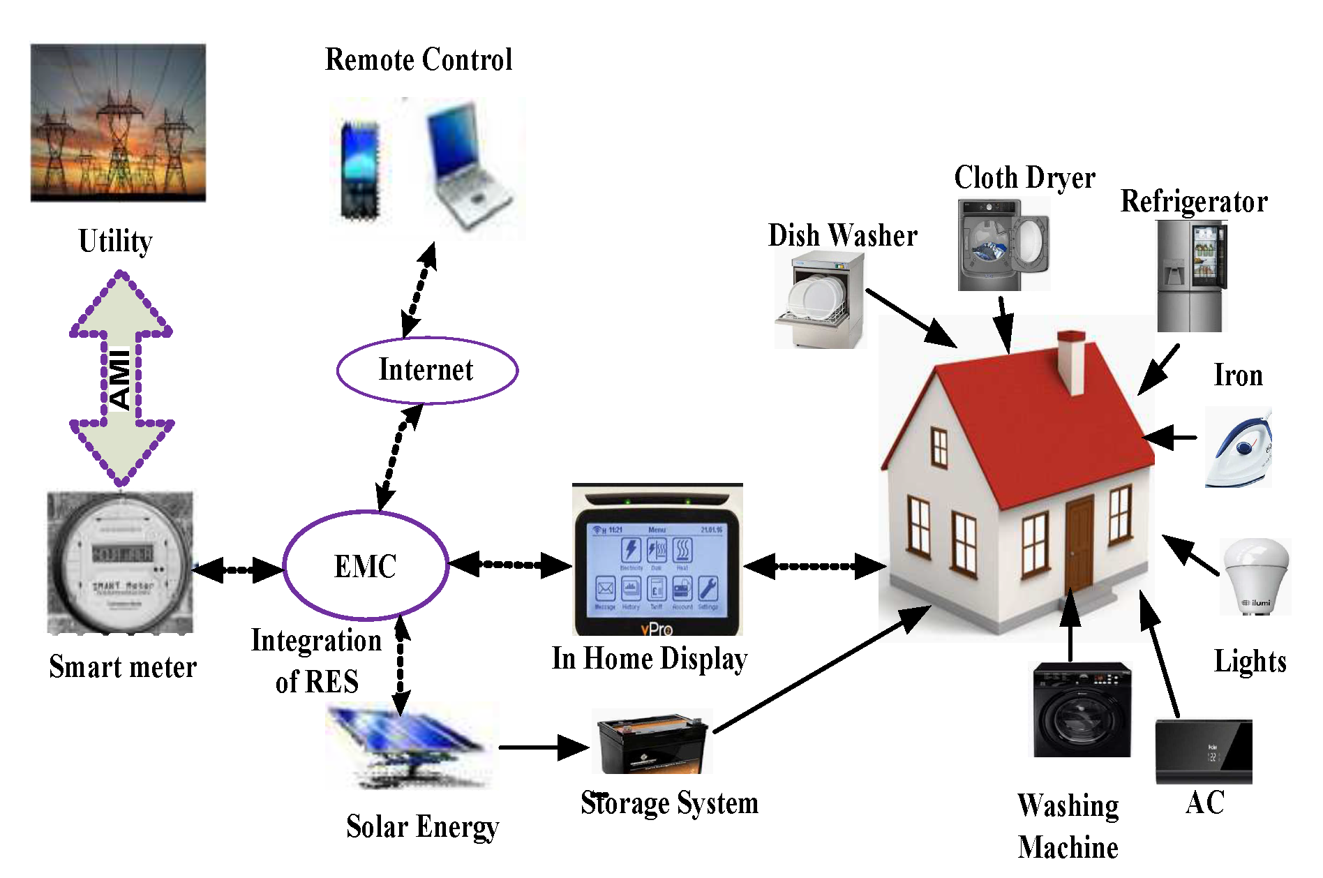
4. System Model
4.1. Categorization of Household Appliances
- Non-interruptible (NI): Appliances such as washing machine and cloth dryer work in a cycle and cannot be interrupted once started and must keep running until the end of their cycles.
- Scheduleable (S): Appliances, i.e., dish washer, iron and vacuum cleaner can be scheduled at any time within given horizon.
- User dependent (UD): Appliances, i.e., lights and fans operate according to user presence; if the user is present, the respective appliance would be turned ON and vice versa.
- Temperature dependent (TD): The working of these appliances, i.e., air-conditioner and refrigerator depend on temperature level. If appliance temperature is low as compared to the specific level, then they will be ON; otherwise, OFF.
4.2. Electricity Pricing Policies
4.2.1. RTP with IBR
5. Integration of RES
5.1. Borowy’s Model of the PV System
6. Problem Formulation
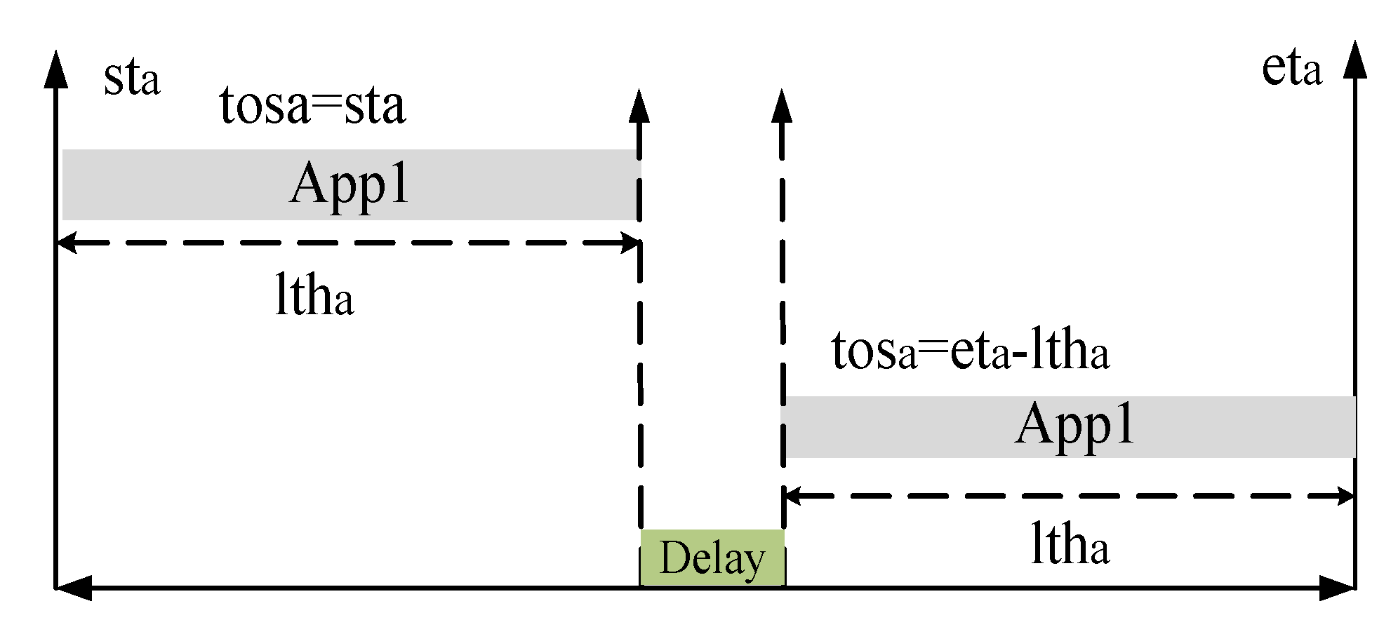
6.1. Delay Factor (DF)
6.2. Impact of Control Parameter on Scheduling
7. Proposed Scheduling Algorithm
| Algorithm 1: The proposed load scheduling optimization algorithm |
 |
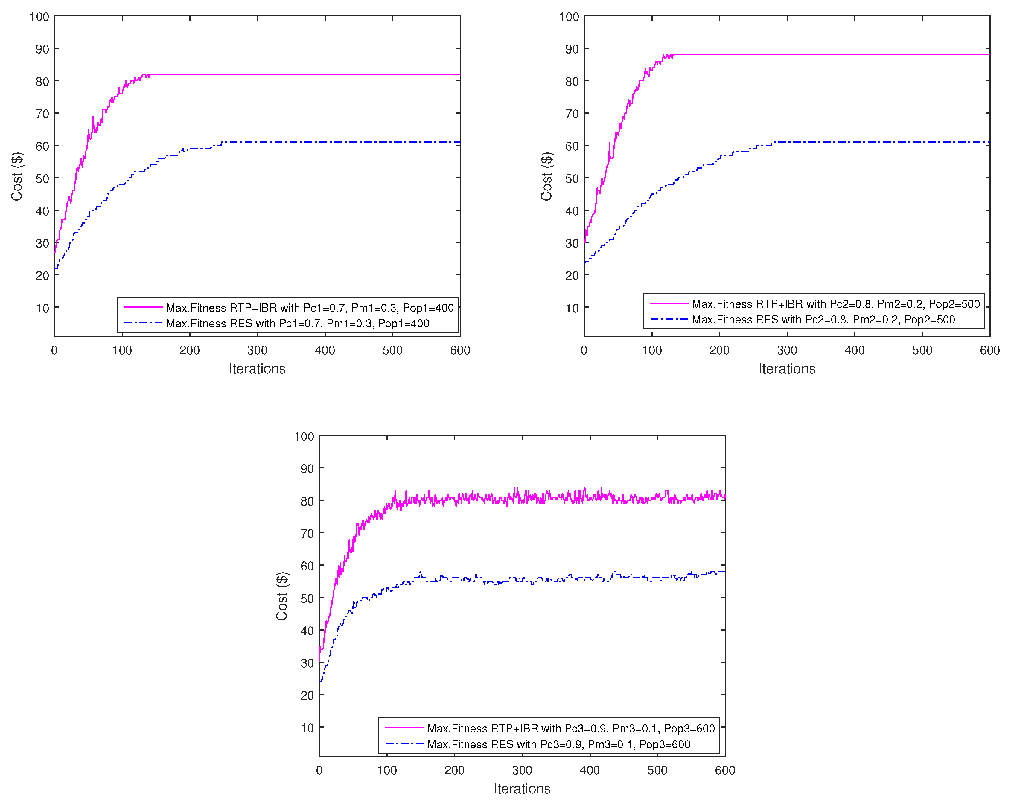
7.1. Convergence Rate of Algorithm
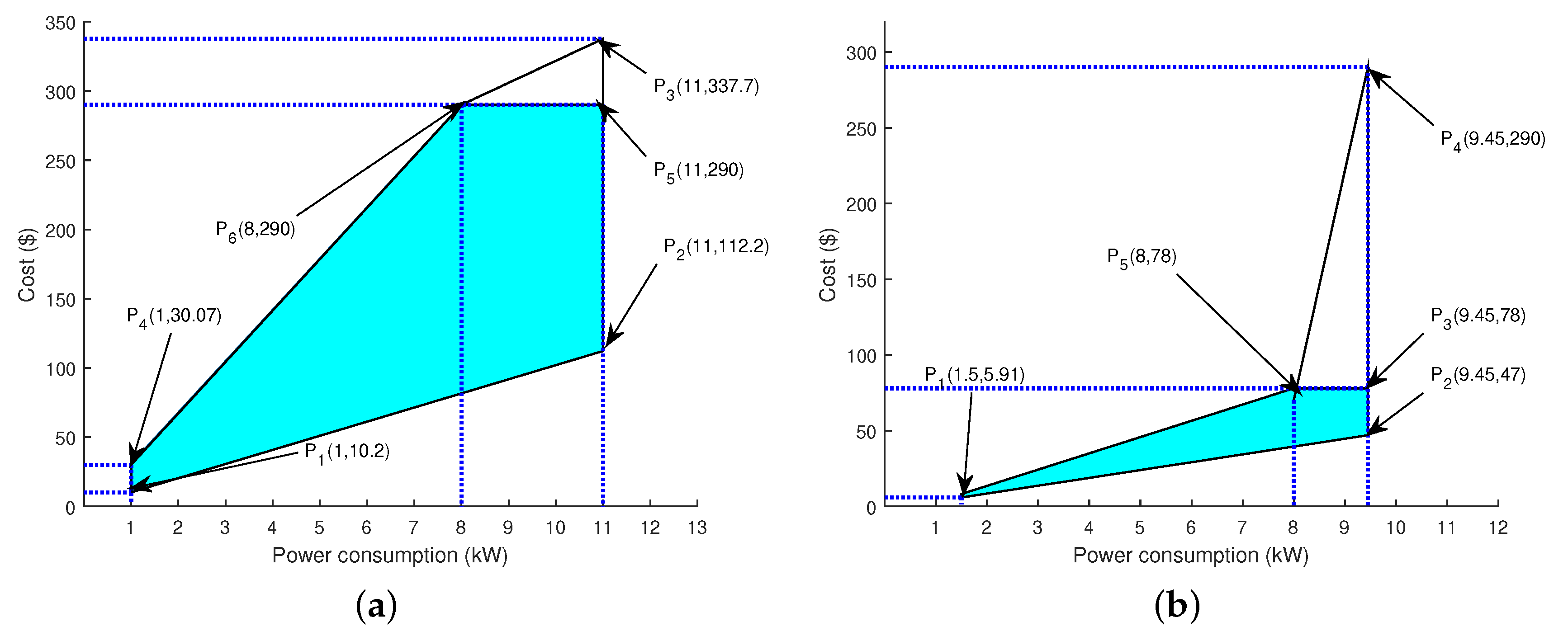
7.2. Feasible Region
7.2.1. Scheduled Load with RTP
7.3. Scheduled Load with RTP+IBR
8. Simulation Results
8.1. Conventional Users
8.2. Smart Users
8.3. Proposed Cases
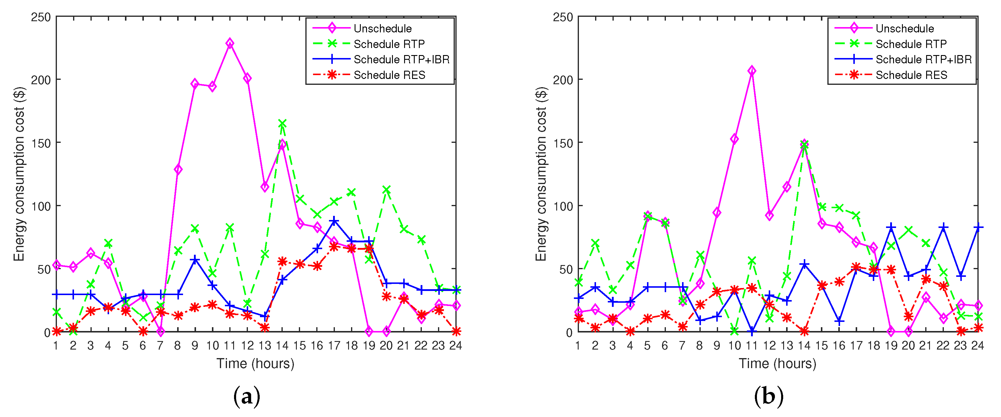
8.3.1. Unscheduled Case
8.3.2. Scheduled Case with RTP
8.3.3. Scheduled Case with RTP+IBR
8.3.4. Scheduled Case with RES
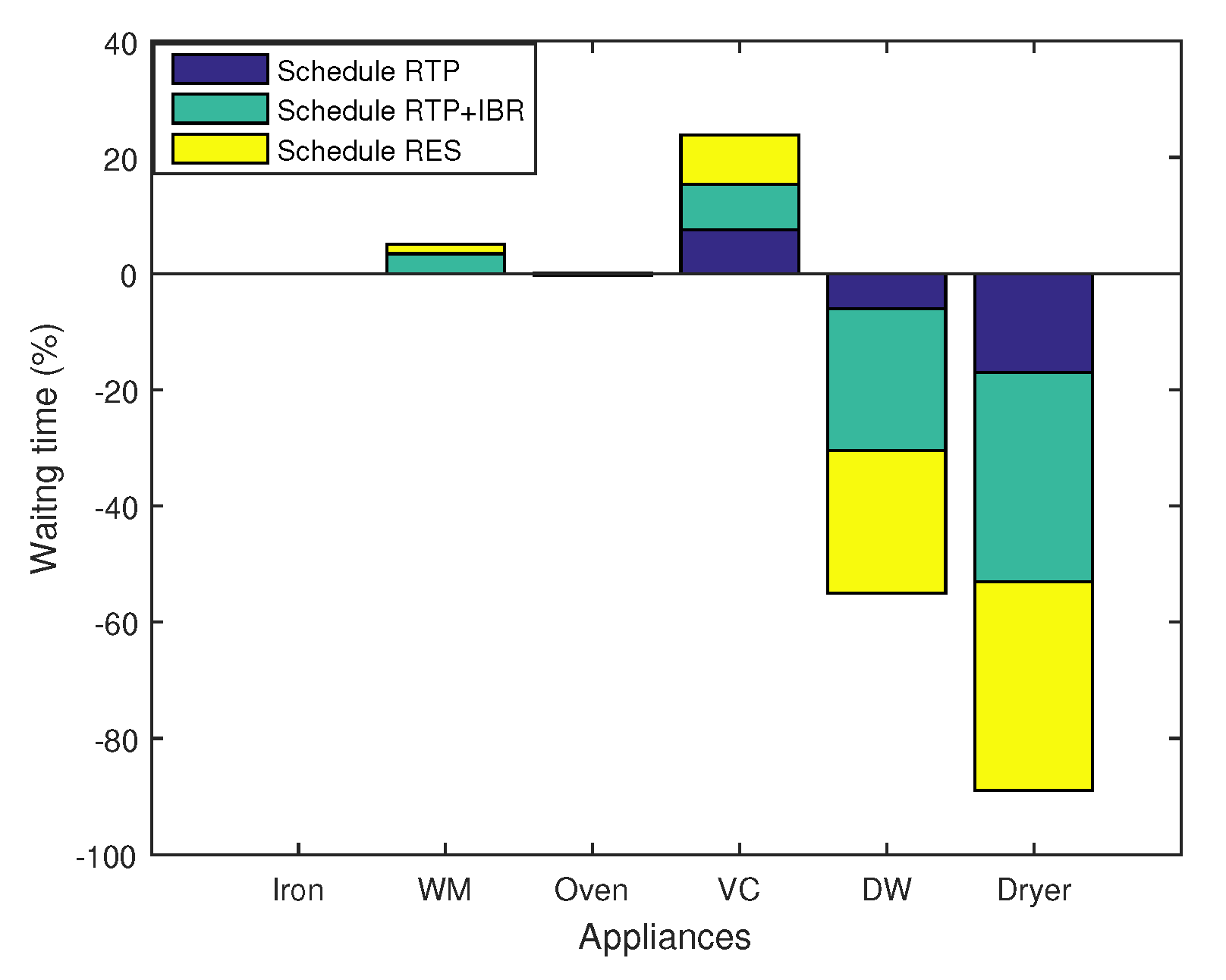
8.3.5. Scheduling Pattern of Appliances
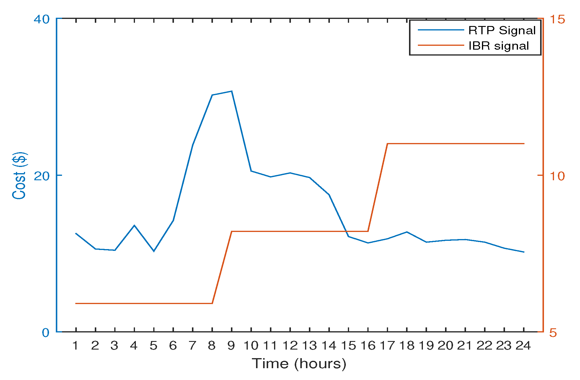
8.4. Pricing Patterns
8.5. Unscheduled Case
8.6. Scheduled Case with RTP
8.7. Scheduled Case with RTP+IBR
8.8. Scheduled Case with RES
8.9. Carbon Footprint
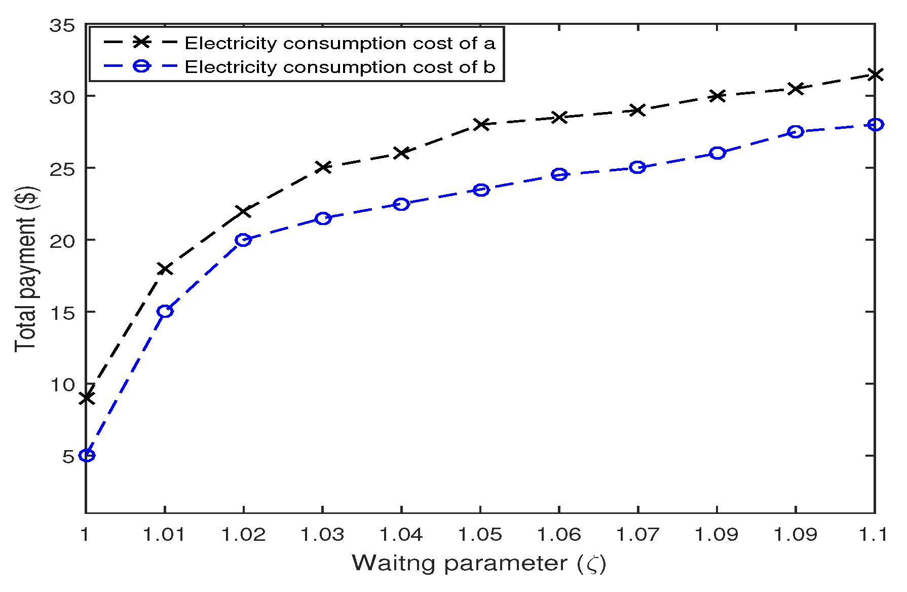
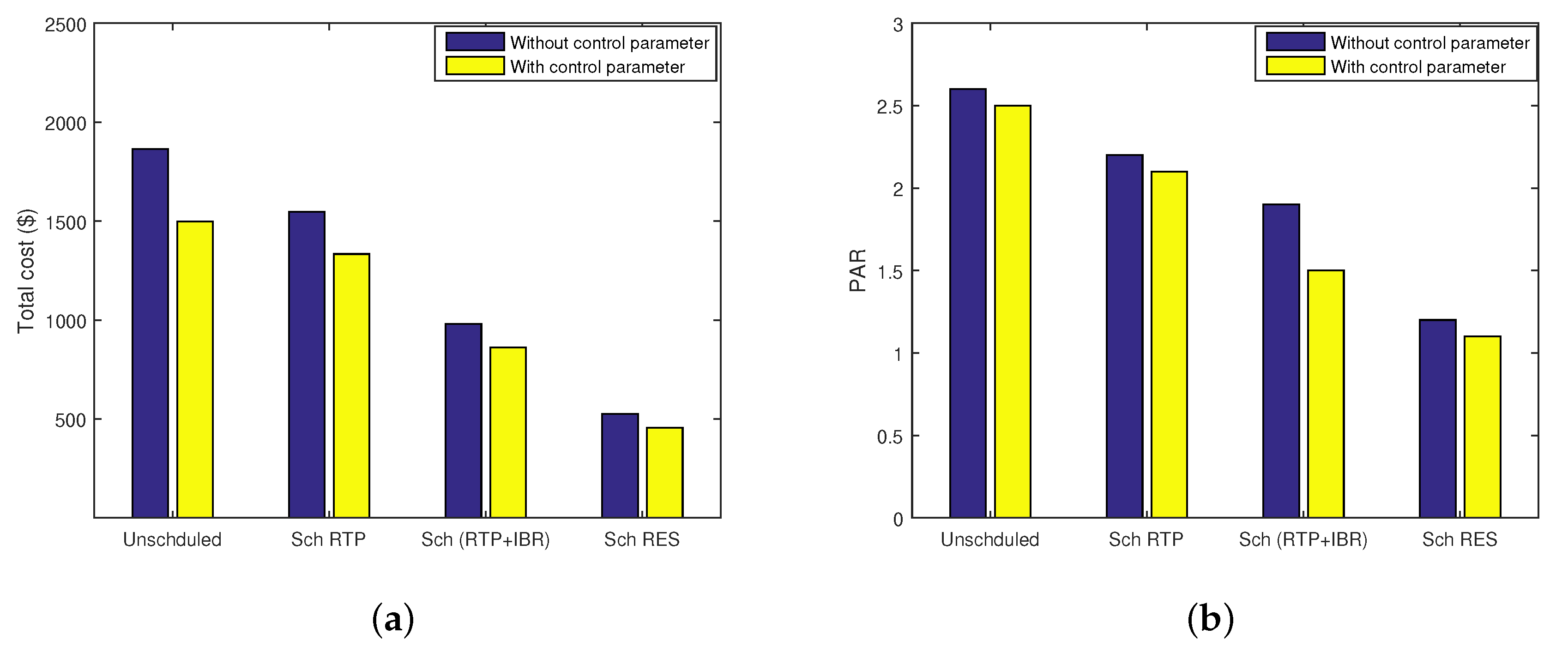
8.10. Trade-Offs
9. Conclusions
Author Contributions
Funding
Conflicts of Interest
References
- Nan, S.; Zhou, M.; Li, G. Optimal residential community demand response scheduling in smart grid. Appl. Energy 2018, 210, 1280–1289. [Google Scholar] [CrossRef]
- Ghorbel, M.B.; Hamdaoui, B.; Guizani, M.; Mohamed, A. Long-Term Power Procurement Scheduling Method for Smart-Grid Powered Communication Systems. IEEE Trans. Wirel. Commun. 2018, 17, 2882–2892. [Google Scholar] [CrossRef]
- Du, Y.F.; Jiang, L.; Li, Y.; Wu, Q. A Robust Optimization Approach for Demand Side Scheduling Considering Uncertainty of Manually Operated Appliances. IEEE Trans. Smart Grid 2018, 9, 743–755. [Google Scholar] [CrossRef]
- Rehmani, M.H.; Reisslein, M.; Rachedi, A.; Erol-Kantarci, M.; Radenkovic, M. Integrating Renewable Energy Resources Into the Smart Grid: Recent Developments in Information and Communication Technologies. IEEE Trans. Ind. Inform. 2018, 14, 2814–2825. [Google Scholar] [CrossRef] [Green Version]
- Cao, Z.; Lin, J.; Wan, C.; Song, Y.; Zhang, Y.; Wang, X. Optimal Cloud Computing Resource Allocation for Demand Side Management in Smart Grid. IEEE Trans. Smart Grid 2017, 8, 1943–1955. [Google Scholar]
- Erdinc, O.; Tascikaraoglu, A.; Paterakis, N.G.; Eren, Y.; Catalao, J. End-user comfort oriented day-ahead planning for responsive residential HVAC demand aggregation considering weather forecasts. In Proceedings of the 2017 IEEE Power & Energy Society General Meeting, Chicago, IL, USA, 16–20 July 2017. [Google Scholar]
- Jindal, A.; Singh, M.; Kumar, N. Consumption-Aware Data Analytical Demand Response Scheme for Peak Load Reduction in Smart Grid. IEEE Trans. Ind. Electron. 2018, 65, 8993–9004. [Google Scholar] [CrossRef]
- Khalid, A.; Javaid, N.; Guizani, M.; Alhussein, M.; Aurangzeb, K.; Ilahi, M. Towards Dynamic Coordination Among Home Appliances Using Multi-Objective Energy Optimization for Demand Side Management in Smart Buildings. IEEE Access 2018, 6, 19509–19529. [Google Scholar] [CrossRef]
- Li, T.; Dong, M. Real-Time Residential-Side Joint Energy Storage Management and Load Scheduling with Renewable Integration. IEEE Trans. Smart Grid 2018, 9, 283–298. [Google Scholar] [CrossRef]
- Huang, H.; Cai, Y.; Xu, H.; Yu, H. A Multiagent Minority-Game-Based Demand-Response Management of Smart Buildings Toward Peak Load Reduction. IEEE Trans. Comput. Aided Des. Integr. Circuits Syst. 2017, 36, 573–585. [Google Scholar] [CrossRef]
- Bollen, M.H.J. Power Quality Concerns in Implementing Smart Distribution-Grid Applications. IEEE Trans. Smart Grid 2017, 8, 391–399. [Google Scholar] [CrossRef]
- Chen, C.; Nagananda, K.G.; Xiong, G.; Kishore, S.; Snyder, L.V. A Communication-Based Appliance Scheduling Scheme for Consumer-Premise Energy Management Systems. IEEE Trans. Smart Grid 2013, 4, 56–65. [Google Scholar] [CrossRef]
- Good, N. A transactive energy modelling and assessment framework for demand response business cases in smart distributed multi-energy systems. Energy 2018. [Google Scholar] [CrossRef]
- Sanjeev, P.; Padhy, N.P.; Agarwal, P. Peak Energy Management Using Renewable Integrated DC Microgrid. IEEE Trans. Smart Grid 2018, 9, 4906–4917. [Google Scholar] [CrossRef]
- Dehghanpour, K.; Nehrir, M.H.; Sheppard, J.W.; Kelly, N.C. Agent-Based Modeling of Retail Electrical Energy Markets With Demand Response. IEEE Trans. Smart Grid 2018, 9, 3465–3475. [Google Scholar] [CrossRef]
- Nguyen, D.H.; Narikiyo, T.; Kawanishi, M. Optimal Demand Response and Real-Time Pricing by a Sequential Distributed Consensus-Based ADMM Approach. IEEE Trans. Smart Grid 2018, 9, 4964–4974. [Google Scholar] [CrossRef]
- Antunes, C.H.; Soares, A.; Gomes, A. An energy management system for residential demand response based on multiobjective optimization. In Proceedings of the 2016 IEEE Smart Energy Grid Engineering (SEGE), Oshawa, ON, USA, 21–24 August 2016; pp. 90–94. [Google Scholar]
- Wang, K.; Li, H.; Maharjan, S.; Zhang, Y.; Guo, S. Green Energy Scheduling for Demand Side Management in the Smart Grid. IEEE Trans. Green Commun. Netw. 2018, 2, 596–611. [Google Scholar] [CrossRef]
- Li, D.; Chiu, W.; Sun, H.; Poor, H.V. Multiobjective Optimization for Demand Side Management Program in Smart Grid. IEEE Trans. Ind. Inform. 2018, 14, 1482–1490. [Google Scholar] [CrossRef]
- Hu, M.; Xiao, J.-W.; Cui, S.-C.; Wang, Y.-W. Distributed real-time demand response for energy management scheduling in smart grid. Int. J. Electr. Power Energy Syst. 2018, 99, 233–245. [Google Scholar] [CrossRef]
- Gottwalt, S.; Garttner, J.; Schmeck, H.; Weinhardt, C. Modeling and Valuation of Residential Demand Flexibility for Renewable Energy Integration. IEEE Trans. Smart Grid 2017, 8, 2565–2574. [Google Scholar] [CrossRef]
- Hayes, B.; Melatti, I.; Mancini, T.; Prodanovic, M.; Tronci, E. Residential Demand Management Using Individualized Demand Aware Price Policies. IEEE Trans. Smart Grid 2017, 8, 1284–1294. [Google Scholar] [CrossRef]
- Keerthisinghe, C.; Verbic, G.; Chapman, A.C. A Fast Technique for Smart Home Management: ADP With Temporal Difference Learning. IEEE Trans. Smart Grid 2018, 9, 3291–3303. [Google Scholar] [CrossRef]
- Asgher, U.; Rasheed, M.B.; Awais, M. Demand Response Benefits for Load Management Through Heuristic Algorithm in Smart Grid. In Proceedings of the IEEE Recent Advances in Electrical Engineering (RAEE), PIEAS, Islamabad, Pakistan, 17–18 October 2018. [Google Scholar]
- Parizy, E.S.; Bahrami, H.R.; Choi, S. A Low Complexity and Secure Demand Response Technique for Peak Load Reduction. IEEE Trans. Smart Grid 2018. [Google Scholar] [CrossRef]
- Huang, X.; Hong, S.H.; Li, Y. Hour-Ahead Price Based Energy Management Scheme for Industrial Facilities. IEEE Trans. Ind. Inform. 2017, 13, 2886–2898. [Google Scholar] [CrossRef]
- Al-sumaiti, A.S.; Ahmed, M.H.; Salama, M.M. Smart home activities: A literature review. Electr. Power Compon. Syst. 2014, 42, 294–305. [Google Scholar] [CrossRef]
- Ejaz, W.; Naeem, M.; Shahid, A.; Anpalagan, A.; Jo, M. Efficient Energy Management for the Internet of Things in Smart Cities. IEEE Commun. Mag. 2017, 55, 84–91. [Google Scholar] [CrossRef] [Green Version]
- Helal, S.A.; Najee, R.J.; Hanna, M.O.; Shaaban, M.F.; Osman, A.H.; Hassan, M.S. On optimal scheduling for smart homes and their integration in smart grids. In Proceedings of the 2017 IEEE 30th Canadian Conference on Electrical and Computer Engineering (CCECE), Windsor, ON, USA, 30 April–3 May 2017; pp. 1–4. [Google Scholar]
- Parisio, A.; Wiezorek, C.; Kyntaja, T.; Elo, J.; Strunz, K.; Johansson, K.H. Cooperative MPC-Based Energy Management for Networked Microgrids. IEEE Trans. Smart Grid 2017, 8, 3066–3074. [Google Scholar] [CrossRef]
- Mehdizadeh, A.; Taghizadegan, N.; Salehi, J. Risk-based energy management of renewable-based microgrid using information gap decision theory in the presence of peak load management. Appl. Energy 2018, 211, 617–630. [Google Scholar] [CrossRef]
- Ma, W.; Wang, J.; Gupta, V.; Chen, C. Distributed Energy Management for Networked Microgrids Using Online ADMM With Regret. IEEE Trans. Smart Grid 2018, 9, 847–856. [Google Scholar] [CrossRef]
- Moon, S.; Lee, J. Multi-Residential Demand Response Scheduling With Multi-Class Appliances in Smart Grid. IEEE Trans. Smart Grid 2018, 9, 2518–2528. [Google Scholar] [CrossRef]
- Cortes-Arcos, T. Multi-objective demand response to real-time prices (RTP) using a task scheduling methodology. Energy 2017, 138, 19–31. [Google Scholar] [CrossRef]
- Fadlullah, Z.M.; Quan, D.M.; Kato, N.; Stojmenovic, I. GTES: An Optimized Game-Theoretic Demand-Side Management Scheme for Smart Grid. IEEE Syst. J. 2014, 8, 588–597. [Google Scholar] [CrossRef] [Green Version]
- Maharjan, S.; Zhu, Q.; Zhang, Y.; Gjessing, S.; Basar, T. Dependable Demand Response Management in the Smart Grid: A Stackelberg Game Approach. IEEE Trans. Smart Grid 2013, 4, 120–132. [Google Scholar] [CrossRef]
- Adika, C.O.; Wang, L. Autonomous Appliance Scheduling for Household Energy Management. IEEE Trans. Smart Grid 2014, 5, 673–682. [Google Scholar] [CrossRef]
- Nunna, H.S.V.S.K.; Battula, S.; Doolla, S.; Srinivasan, D. Energy Management in Smart Distribution Systems With Vehicle-to-Grid Integrated Microgrids. IEEE Trans. Smart Grid 2018, 9, 4004–4016. [Google Scholar] [CrossRef]
- Hosen, M.A.; Khosravi, A.; Nahavandi, S.; Creighton, D. Improving the Quality of Prediction Intervals Through Optimal Aggregation. IEEE Trans. Ind. Electron. 2015, 62, 4420–4429. [Google Scholar] [CrossRef]
- Saadat, J.; Moallem, P.; Koofigar, H. Training Echo State Neural Network Using Harmony Search Algorithm. Int. J. Artif. Intell. 2017, 15, 163–179. [Google Scholar]
- Precup, R.; David, R.; Petriu, E.M. Grey Wolf Optimizer Algorithm-Based Tuning of Fuzzy Control Systems With Reduced Parametric Sensitivity. IEEE Trans. Ind. Electron. 2017, 64, 527–534. [Google Scholar] [CrossRef]
- Vrkalovic, S.; Lunca, E.C.; Borlea, I.D. Model-free sliding mode and fuzzy controllers for reverse osmosis desalination plants. Int. J. Artif. Intell. 2018, 16, 208–222. [Google Scholar]
- Wu, X.; Hu, X.; Yin, X.; Moura, S.J. Stochastic Optimal Energy Management of Smart Home With PEV Energy Storage. IEEE Trans. Smart Grid 2018, 9, 2065–2075. [Google Scholar] [CrossRef]
- Celik, B.; Roche, R.; Bouquain, D.; Miraoui, A. Decentralized neighborhood energy management with coordinated smart home energy sharing. IEEE Trans. Smart Grid 2018, 9, 6387–6397. [Google Scholar]
- Park, L.; Jang, Y.; Cho, S.; Kim, J. Residential Demand Response for Renewable Energy Resources in Smart Grid Systems. IEEE Trans. Ind. Inform. 2017, 13, 3165–3173. [Google Scholar] [CrossRef]
- Keles, C.; Alagoz, B.B.; Kaygusuz, A. Multi-source energy mixing for renewable energy microgrids by particle swarm optimization. In Proceedings of the 2017 International Artificial Intelligence and Data Processing Symposium (IDAP), Malatya, Turkey, 16–17 September 2017; pp. 1–5. [Google Scholar]
- Wen, Z.; Neill, D.O.; Maei, H. Optimal Demand Response Using Device-Based Reinforcement Learning. IEEE Trans. Smart Grid 2015, 6, 2312–2324. [Google Scholar] [CrossRef]
- Vardakas, J.S.; Zorba, N.; Verikoukis, C.V. Power demand control scenarios for smart grid applications with finite number of appliances. Appl. Energy 2016, 162, 83–98. [Google Scholar] [CrossRef] [Green Version]
- Li, C.; Yu, X.; Yu, W.; Chen, G.; Wang, J. Efficient Computation for Sparse Load Shifting in Demand Side Management. IEEE Trans. Smart Grid 2017, 8, 250–261. [Google Scholar] [CrossRef]
- El Shafie, A.; Niyato, D.; Hamila, R.; Al-Dhahir, N. Impact of the Wireless Network’s PHY Security and Reliability on Demand-Side Management Cost in the Smart Grid. IEEE Access 2017, 5, 5678–5689. [Google Scholar] [CrossRef]
- Kim, S.J.; Giannakis, G.B. Scalable and Robust Demand Response With Mixed-Integer Constraints. IEEE Trans. Smart Grid 2013, 4, 2089–2099. [Google Scholar]
- Werminski, S. Demand side management using DADR automation in the peak load reduction. Renew. Sustain. Energy Rev. 2017, 67, 998–1007. [Google Scholar] [CrossRef]
- Aktas, A. Experimental investigation of a new smart energy management algorithm for a hybrid energy storage system in smart grid applications. Electr. Power Syst. Res. 2017, 144, 185–196. [Google Scholar] [CrossRef]
- Alkaabi, S.S.; Zeineldin, H.H.; Khadkikar, V. Short-Term Reactive Power Planning to Minimize Cost of Energy Losses Considering PV Systems. IEEE Trans. Smart Grid 2018. [Google Scholar] [CrossRef]
- Bao, Z. Optimal Multi-Timescale Demand Side Scheduling Considering Dynamic Scenarios of Electricity Demand. IEEE Trans. Smart Grid 2018. [Google Scholar] [CrossRef]
- Zhao, B. Energy Management of Multiple-Microgrids based on a System of Systems Architecture. IEEE Trans. Power Syst. 2018. [Google Scholar] [CrossRef]
- Mortazavi, H.; Mehrjerdi, H.; Saad, M.; Lefebvre, S. Distribution power factor monitoring in presence of high RES integration using a modified load encroachment technique. IET Renew. Power Gener. 2018, 12, 851–858. [Google Scholar] [CrossRef]
- Huang, C.; Wang, L.; Yeung, R.S.; Zhang, Z.; Chung, H.S.; Bensoussan, A. A Prediction Model-Guided Jaya Algorithm for the PV System Maximum Power Point Tracking. IEEE Trans. Sustain. Energy 2018, 9, 45–55. [Google Scholar] [CrossRef]
- Kivimäki, J.; Kolesnik, S.; Sitbon, M.; Suntio, T.; Kuperman, A. Design Guidelines for Multiloop Perturbative Maximum Power Point Tracking Algorithms. IEEE Trans. Power Electron. 2018, 33, 1284–1293. [Google Scholar] [CrossRef]
- Al-Sumaiti, A.S.; Ahmed, M.H.; Salama, M. Residential Load Management Under Stochastic Weather Condition in Developing Countries. Electr. Power Components Syst. 2014, 42, 1452–1473. [Google Scholar] [CrossRef]
- Javaid, N.; Naseem, M.; Rasheed, M.B.; Mahmood, D.; Khan, S.A.; Alrajeh, N.; Iqbal, Z. A new heuristically optimized Home Energy Management controller for smart grid. Sustain. Cities Soc. 2017, 34, 211–227. [Google Scholar] [CrossRef]
- Rasheed, M.B.; Javaid, N.; Imran, M.; Khan, Z.A.; Qasim, U.; Vasilakos, A. Delay and energy consumption analysis of priority guaranteed MAC protocol for wireless body area networks. Wirel. Netw. 2017, 23, 1249–1266. [Google Scholar] [CrossRef]
- Elghitani, F.; Zhuang, W. Aggregating a Large Number of Residential Appliances for Demand Response Applications. IEEE Trans. Smart Grid 2018, 9, 5092–5100. [Google Scholar] [CrossRef]
- Lizondo, D.; Rodriguez, S.; Will, A.; Jimenez, V.; Gotay, J. An Artificial Immune Network for Distributed Demand-Side Management in Smart Grids. Inf. Sci. 2018, 438, 32–45. [Google Scholar] [CrossRef]
- Liu, R.-S.; Hsu, Y.-F. A scalable and robust approach to demand side management for smart grids with uncertain renewable power generation and bi-directional energy trading. Int. J. Electr. Power Energy Syst. 2018, 97, 396–407. [Google Scholar] [CrossRef]
- Tushar, M.H.K.; Zeineddine, A.W.; Assi, C. Demand-Side Management by Regulating Charging and Discharging of the EV, ESS, and Utilizing Renewable Energy. IEEE Trans. Ind. Inform. 2018, 14, 117–126. [Google Scholar] [CrossRef]
- Bui, V.; Hussain, A.; Kim, H. A Multiagent-Based Hierarchical Energy Management Strategy for Multi-Microgrids Considering Adjustable Power and Demand Response. IEEE Trans. Smart Grid 2018, 9, 1323–1333. [Google Scholar] [CrossRef]
- Zhao, Z.; Lee, W.C.; Shin, Y.; Song, K. An Optimal Power Scheduling Method for Demand Response in Home Energy Management System. IEEE Trans. Smart Grid 2013, 4, 1391–1400. [Google Scholar] [CrossRef]
- Luo, C.; Huang, Y.; Gupta, V. Stochastic Dynamic Pricing for EV Charging Stations With Renewable Integration and Energy Storage. IEEE Trans. Smart Grid 2018, 9, 1494–1505. [Google Scholar] [CrossRef] [Green Version]
- Baronti, F.; Vazquez, S.; Chow, M. Modeling, Control, and Integration of Energy Storage Systems in E-Transportation and Smart Grid. IEEE Trans. Ind. Electron. 2018, 65, 6548–6551. [Google Scholar] [CrossRef]
- Kadri, R.L.; Boctor, F.F. An efficient genetic algorithm to solve the resource-constrained project scheduling problem with transfer times: The single mode case. Eur. J. Oper. Res. 2018, 265, 454–462. [Google Scholar] [CrossRef]
- Gong, D.; Sun, J.; Miao, Z. A Set-Based Genetic Algorithm for Interval Many-Objective Optimization Problems. IEEE Trans. Evol. Comput. 2018, 22, 47–60. [Google Scholar] [CrossRef]
- Abushnaf, J.; Rassau, A. Impact of energy management system on the sizing of a grid-connected PV/Battery system. Electr. J. 2018, 31, 58–66. [Google Scholar] [CrossRef]
- Yaagoubi, N.; Mouftah, H.T. User-Aware Game Theoretic Approach for Demand Management. IEEE Trans. Smart Grid 2015, 6, 716–725. [Google Scholar] [CrossRef]
- Rasheed, M.B.; Javaid, N.; Ahmad, A.; Awais, M.; Khan, Z.A.; Qasim, U.; Alrajeh, N. Priority and delay constrained demand side management in real-time price environment with renewable energy source. Int. J. Energy Res. 2016, 40, 2002–2021. [Google Scholar] [CrossRef]
- Chen, W.-H.; Wu, P.-H.; Lin, Y.-L. Performance optimization of thermoelectric generators designed by multi-objective genetic algorithm. Appl. Energy 2018, 209, 211–223. [Google Scholar] [CrossRef]
- Moreno, J.; Lopez, M.A.; Martinez, R. A new algorithm for solving all the real roots of a nonlinear system of equations in a given feasible region. Numer. Algor. 2018, 1–32. [Google Scholar] [CrossRef]
- Time has Arrived for Time Variant Pricing, but What Kind? Available online: http://www.menloenergy.com/?p=349 (accessed on 23 August 2018).
- Askarzadeh, A. A Memory-Based Genetic Algorithm for Optimization of Power Generation in a Microgrid. IEEE Trans. Sustain. Energy 2018, 9, 1081–1089. [Google Scholar] [CrossRef]
- Energy Market and Operational Data. Available online: http://mis.nyiso.com/public/pdf/damlbmp/20181214damlbmp_zone.pdf (accessed on 12 May 2018).


| References | Techniques | Objective(s) | Achievement(s) | Limitation(s) | RESs |
|---|---|---|---|---|---|
| [25] | LP | Balance the daily demand that minimize the peaks | Efficiently overcomes the peak hour load | Time complexity | No |
| [26] | PSO and DAP | Limit the power consumption | Reduces the consumption cost | User comfort not considered | No |
| [28,29] | TS and EDE | Schedule the daily load for cost reduction | Better scheduling is achieved for minimum cost | User comfort is neglected | No |
| [30] | BFOA and BA | Maximize the profit | Optimal scheduling of household energy demand | Slow convergence rate | No |
| [31] | MILP and GA | Overcome the cost and peak load | Minimized the delay time of appliances and cost | Increased complexity of system | No |
| [18,32] | CC and DADR algorithm | Increase user comfort and minimize delay time | It efficiently reduces the peak load at the grid to a great extent | Big data management and fault tolerance issues in real time rate increases drastically | No |
| [33] | DE and PSO | User frustration and electricity bill reduction | Minimized electricity bill | Low energy consumption users are affected | No |
| [34,35] | RLS | Scheduling based on forecasting price and cost minimization | Minimizing peak cost and increasing user satisfaction | Delay cost not considered | No |
| [36,37] | Quasi random process | Peak demand valuation without considering number of appliances | Recursive method is used for load scheduling for peak demand achievement | User comfort and peak demand is not considered which may cause overburden utility | No |
| [38] | Pareto optimality | System reliability & security analysis in DSM | Enhanced the reliability of power system | System reliability in terms of outage failure cost not considered | No |
| References | Techniques | Objective(s) | Achievement(s) | Limitations | RES |
|---|---|---|---|---|---|
| [45,46] | ACO | Single and multiple home appliance scheduling using knapsack problem | Minimize cost, and maximize comfort with RES | RES installation cost is not calculated | Yes |
| [47,48] | PSO | To find out optimal energy mixing rates that can minimize daily energy cost of a renewable MGs with RESs | Reduction in cost and discomfort | low convergence rate of algorithm | Yes |
| [49,50] | NE and NM | Sparse load interruption with increment in convergence rate | Minimize the customer discomfort and achieved better convergence rate | The cost of peak hours are not minimized and PAR not considered | Yes |
| [51] | C&CG and SRDSM algorithms | Cost minimization with RESs and batteries | Minimize the cost of all consumers | Only considers the total load cost, peak cost are ignored and overall cost of system is increased | Yes |
| [52,53] | MPPT algorithm | Energy storage with the integration of RESs by using HESS. | Increase the efficiency of batteries from high frequency of ripple currents | Increased the overall system cost | Yes |
| [54,55] | NLP and OPF | Cost minimization with PV inverters | Impressive cost reduction | Increase system complexity | Yes |
| [56,57] | Optimal multi timescale technique | Week-ahead DSM scheduling | Accomplishing the ideal DSM conspire with the questionable client power request | User priority is ignored | No |
| [58,59] | C&CG | Coordination of distributed generation units within individual MGs | Daily energy demand cost is reduced | C&CG is an iterative method so time complexity is increased | Yes |
| [16] | Nash theorem | Minimize the electricity and electric vehicles (EV) cost | Achieved the balance load demand and integration of EV with RESs | User delay cost not calculated | Yes |
| Category | Appliances | LOT (h.) | Power Ratings (KWh) |
|---|---|---|---|
| NI | Load1 | 5 | 2 |
| Load2 | 11 | 1 | |
| S | Load3 | 8 | 2.5 |
| Load4 | 8 | 3.5 | |
| UD | Load5 | 14 | 0.5 |
| TD | Load6 | 7 | 2.5 |
| Parameters | Values |
|---|---|
| Number of appliances | 6 |
| Max. generation | 500 |
| Population size | 400 |
| Pc | 0.8 |
| Pm | 0.2 |
| Event | Load (KWh) | EP ($/KWh) | Cost ($) |
|---|---|---|---|
| Min- load, Min-EP | 1 | 10.2 | 10.2 |
| Min- load, Max-EP | 1 | 30.7 | 30.7 |
| Max- load, Min-EP | 11 | 10.2 | 112.2 |
| Max- load, Max-EP | 11 | 30.7 | 337.7 |
| Event | Load (KWh) | EP ($/KWh) | Cost ($) |
|---|---|---|---|
| Min-load, Min-EP | 1.5 | 10.2 | 15.3 |
| Min-load, Max-EP | 1.5 | 30.7 | 46.50 |
| Max-load, Min-EP | 9.45 | 10.2 | 112.2 |
| Max-load, Max-EP | 9.45 | 30.7 | 290.11 |
| Category | Energy (KWh) | Cost ($) | Cost (%) | Carbon Footprint (metric tons) |
|---|---|---|---|---|
| Unsch. case | 111.5 | 1860 | 38 | 104.81 |
| Sch. with RTP case | 111.5 | 1130 | 34 | 104.81 |
| Sch. with RTP+IBR case | 111.5 | 619.34 | 17 | 104.81 |
| Sch. with RES case | 690.56 | 604.39 | 11 | 98.2 |
| Parameters | Unsch. | Sch. RTP | Savings | Sch. RTP+IBR | Savings | Sch. RES | Savings | Unsch. with | Sch. RTP with | Savings | Sch. RTP+IBR with | Savings | Sch. RES with | Savings |
|---|---|---|---|---|---|---|---|---|---|---|---|---|---|---|
| Per hour cost | 228 | 165 | 72 % | 88 | 38.6% | 57 | 25% | 206.5 | 121.8 | 59% | 82 | 39.6% | 51 | 24.6% |
| Total cost | 1864 | 1547 | 83% | 980 | 52.6% | 526 | 28% | 1498 | 1334 | 89% | 862 | 57% | 456 | 30% |
| PAR | 2.68 | 2.2 | 82% | 1.93 | 72% | 1.23 | 45.9% | 2.5 | 2.1 | 84% | 1.5 | 55.9% | 1.12 | 44.8% |
© 2018 by the authors. Licensee MDPI, Basel, Switzerland. This article is an open access article distributed under the terms and conditions of the Creative Commons Attribution (CC BY) license (http://creativecommons.org/licenses/by/4.0/).
Share and Cite
Asgher, U.; Babar Rasheed, M.; Al-Sumaiti, A.S.; Ur-Rahman, A.; Ali, I.; Alzaidi, A.; Alamri, A. Smart Energy Optimization Using Heuristic Algorithm in Smart Grid with Integration of Solar Energy Sources. Energies 2018, 11, 3494. https://doi.org/10.3390/en11123494
Asgher U, Babar Rasheed M, Al-Sumaiti AS, Ur-Rahman A, Ali I, Alzaidi A, Alamri A. Smart Energy Optimization Using Heuristic Algorithm in Smart Grid with Integration of Solar Energy Sources. Energies. 2018; 11(12):3494. https://doi.org/10.3390/en11123494
Chicago/Turabian StyleAsgher, Urooj, Muhammad Babar Rasheed, Ameena Saad Al-Sumaiti, Atiq Ur-Rahman, Ihsan Ali, Amer Alzaidi, and Abdullah Alamri. 2018. "Smart Energy Optimization Using Heuristic Algorithm in Smart Grid with Integration of Solar Energy Sources" Energies 11, no. 12: 3494. https://doi.org/10.3390/en11123494