A MBCRF Algorithm Based on Ensemble Learning for Building Demand Response Considering the Thermal Comfort

Abstract
:1. Introduction
- A set of linguistic if-then rules are used to form the candidate features during the process of a learning expected tree model, and then the approach on the basis of variable importance is utilized for the feature selection.
- An ensemble learning algorithm, random forest (RF), is selected to estimate the baseline electricity demands. Compared with other learning methods, the prediction error of RF can be as low as 1.28%.
- A novel model based control with a random forest (MBCRF) learning algorithm is developed for the optimal DR control strategies. Based on the proposed MBCRF algorithm, multiple model trees are built and the energy consumption model is fitted in their leaves.
2. Problem Formulation
2.1. Baseline Load Prediction
2.2. DR Strategy Programming
3. Mathematical Preliminaries
3.1. Classification and Regression Tree
3.2. Random Forest
4. The Proposed MBCRF Algorithm
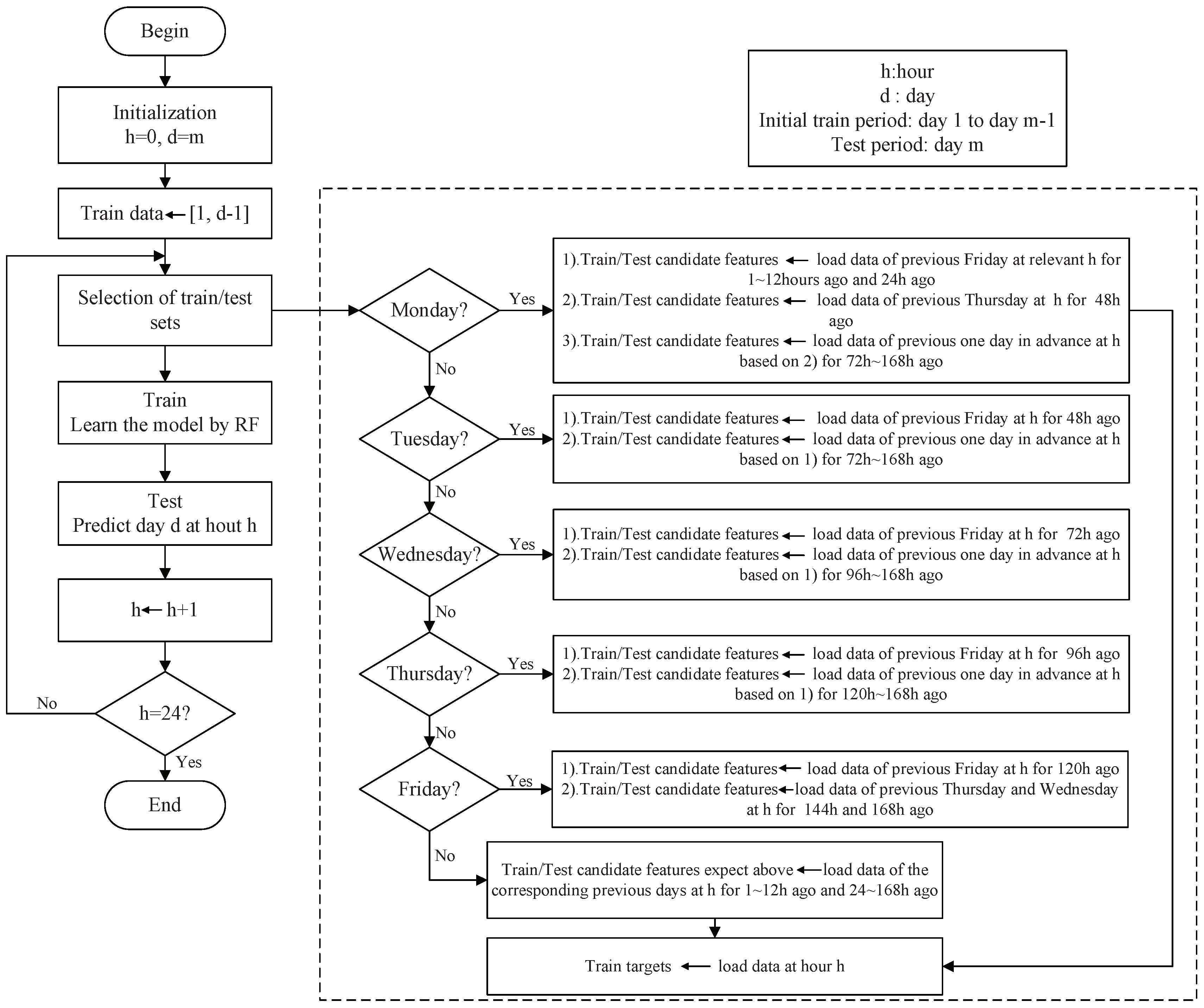
4.1. Overview Flow
4.2. Modeling Candidate Features
4.3. Splitting Feature Selection Based on Variable Importance
4.4. The Proposed MBCRF Algorithm
| Algorithm 1 MBCRF algorithm for the DR optimal strategy. |
| 1: procedure Model learning 2: Select input features 3: 4: 5: Build the MBCRF power prediction tree with 6: for all Regions at the leaves of do 7: Fit linear model 8: end for 9: end procedure 10: procedure Control strategy solving 11: Before time t of DR event, using forecast determine the leaf for 12: Fit the linear model at the leaf 13: Solve optimization in Equation (16) to obtain optimal control strategy 14: end procedure |
4.5. Parameter in MBCRF
- (1)
- The number of trees in the forest, .
- (2)
- The number of splitting features randomly selected from the feature set which are tried for searching the best splitting feature at each internal node, .
- (3)
- The minimum number of a leaf node, .
5. Case Study
5.1. Simulation Data
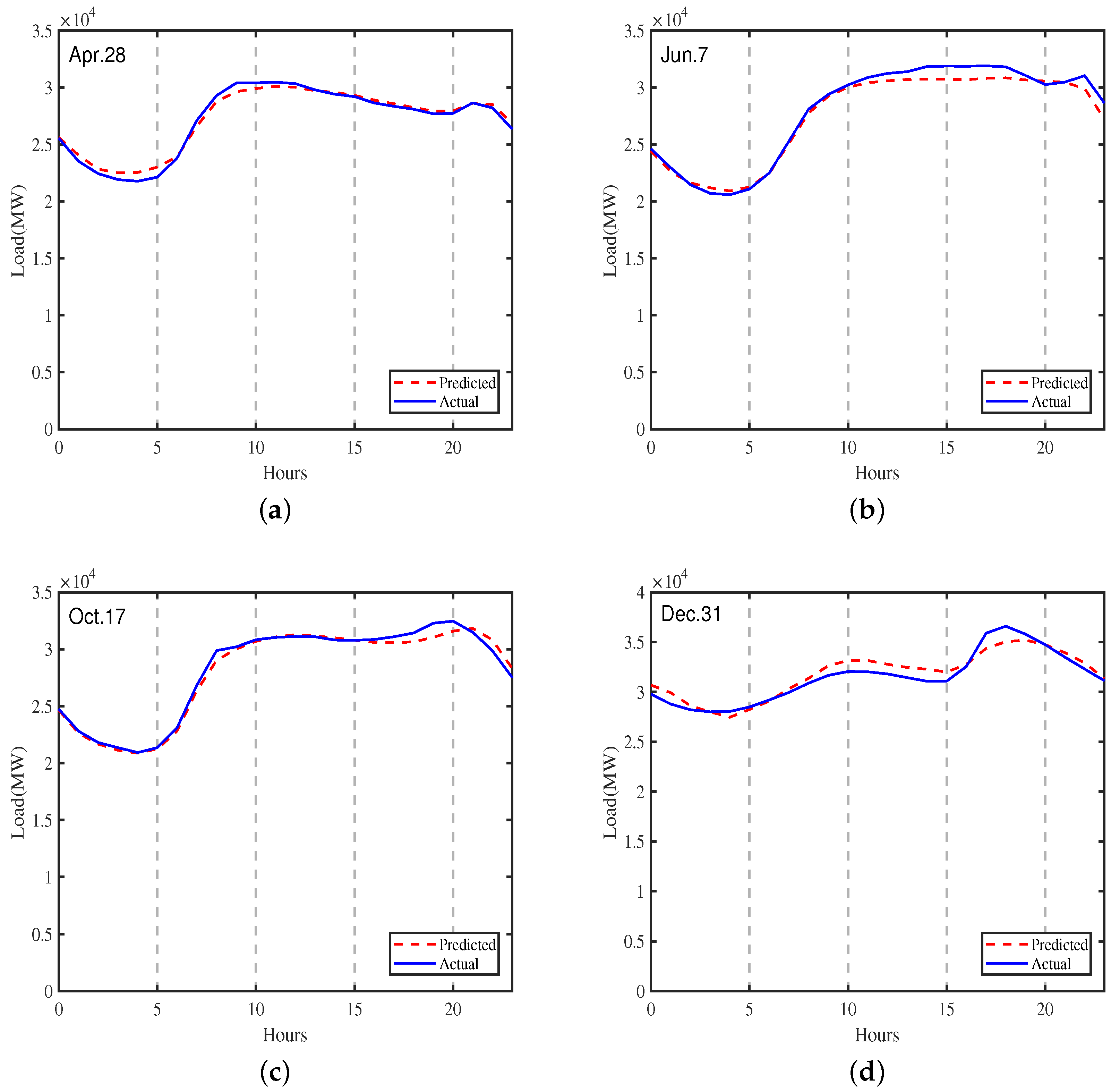
5.2. Load Prediction Benchmarking
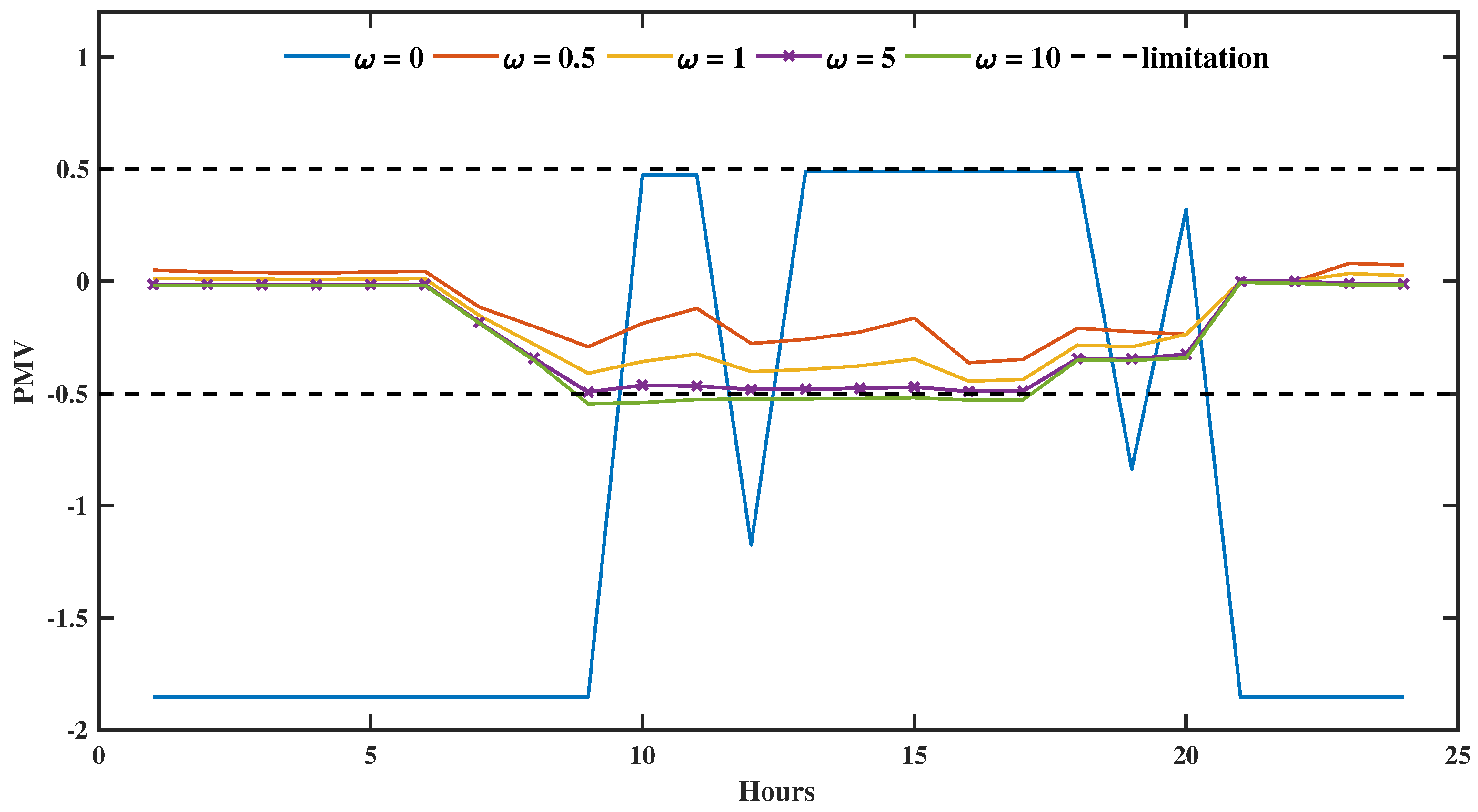
5.3. DR Strategy Optimization
6. Conclusions and Future Work
Author Contributions
Funding
Conflicts of Interest
Nomenclature
| Abbreviations | |
| DR | demand response |
| HVAC | heating, ventilation and air-conditioning |
| CSP | curtailment service provider |
| IBP | incentive-based program |
| PBP | price-based program |
| DLC | direct load control |
| I/C | interruptible/curtailable |
| TOU | time of use |
| CPP | critical peak pricing |
| RTP | real time pricing |
| RL | reinforcement learning |
| CART | classification and regression tree |
| RF | random forest |
| OOB | out-of-bag |
| OOBError | out-of-bag error |
| VIM | variable importance measurement |
| MAPE | mean absolute percentage error |
| MBCRF | model based control with random forest |
| STLF | short-term load forecasting |
| ICT | information communication technology |
| PJM | Pennsylvania–Jersey–Maryland |
| NREL | National Renewable Energy Laboratory |
| RSF | research and support facility |
| ANN | artificial neural network |
| SVR | support vector regression |
| MLR | multiple linear regression |
| PMV | predicted mean vote |
| Variables & Parameters | |
| estimation of baseline load | |
| predicted power response in DR programming | |
| feature vector i of a training set | |
| d-th feature in a feature vector | |
| label of sample i, for the case of STLF, is the actual load | |
| predicted of sample i, for the case of STLF, is the predicted load | |
| the load at time | |
| k type temperature at time t | |
| expected set-point of temperature | |
| day-ahead electricity price at time t | |
| set of controllable variables | |
| set of disturbance variables | |
| set of optimal decision variables | |
| fitting coefficients | |
| weight of thermal comfort | |
| lower bound of power consumption | |
| upper bound of power consumption | |
| number of trees in the forest | |
| number of splitting features in the forest | |
| minimum number of leaf nodes | |
References
- Christantoni, D.; Oxizidis, S.; Flynn, D.; Finn, D.P. Implementation of demand response strategies in a multi-purpose commercial building using a whole-building simulation model approach. Energy Build. 2016, 131, 76–86. [Google Scholar] [CrossRef]
- DOE US. Buildings Energy Data Book; DOE US: Washington, DC, USA, 2013.
- Gao, D.C.; Sun, Y.J. A GA-based coordinated demand response control for building group level peak demand limiting with benefits to grid power balance. Energy Build. 2016, 110, 31–40. [Google Scholar] [CrossRef]
- Federal Energy Regulatory Commission. Assessment of Demand Response and Advanced Metering; Federal Energy Regulatory Commission: Washington, DC, USA, 2012.
- Shariatzadeh, F.; Mandal, P.; Srivastava, A.K. Demand response for sustainable energy systems: A review, application and implementation strategy. Renew. Sust. Energy Rev. 2015, 45, 343–350. [Google Scholar] [CrossRef]
- Xue, X.; Wang, S.W.; Yan, C.C.; Cui, B.R. A fast chiller power demand response control strategy for buildings connected to smart grid. Appl. Energy 2015, 137, 77–87. [Google Scholar] [CrossRef]
- Goddard, G.; Klose, J.; Backhaus, S. Model development and identification for fast demand response in commercial HVAC systems. IEEE Trans. Smart Grid 2014, 5, 2084–2092. [Google Scholar] [CrossRef]
- Ma, Z.; Billanes, J.D.; Jørgensen, B.N. Aggregation potentials for buildings—business models of demand response and virtual power plants. Energies 2017, 10, 1646. [Google Scholar] [CrossRef]
- Khan, A.R.; Mahmood, A.; Safdar, A.; Khan, Z.A. Load forecasting, dynamic pricing and DSM in smart grid: A review. IEEE Trans. Smart Grid 2016, 54, 1311–1322. [Google Scholar] [CrossRef]
- Ji, H.Y.; Baldick, R.; Novoselac, A. Dynamic demand response controller based on real-time retail price for residential buildings. IEEE Trans. Smart Grid 2014, 5, 121–129. [Google Scholar] [CrossRef]
- Asadinejad, A.; Tomsovic, K. Optimal use of incentive and price based demand response to reduce costs and price volatility. Electr. Power Syst. Res. 2017, 144, 215–223. [Google Scholar] [CrossRef]
- Gao, D.C.; Sun, Y.; Lu, Y. A robust demand response control of commercial buildings for smart grid under load prediction uncertainty. Energy 2015, 93, 275–283. [Google Scholar] [CrossRef]
- Samadi, P.; Mohsenian-Rad, H.; Wong, V.W.S.; Schober, R. Tackling the load uncertainty challenges for energy consumption scheduling in smart grid. IEEE Trans. Smart Grid 2013, 4, 1007–1016. [Google Scholar] [CrossRef]
- Dupont, B.; Dietrich, K.; Jonghe, C.D.; Ramos, A.; Belmans, R.; Dong, F.G. Impact of residential demand response on power system operation: A Belgian case study. Appl. Energy 2014, 122, 1–10. [Google Scholar] [CrossRef]
- Beil, I.; Hiskens, I.; Backhaus, S. Frequency regulation from commercial building HVAC demand response. Proc. IEEE 2016, 104, 745–757. [Google Scholar] [CrossRef]
- Zhou, Z.; Zhao, F.; Wang, J. Agent-based electricity market simulation with demand response from commercial buildings. IEEE Trans. Smart Grid 2011, 2, 580–588. [Google Scholar] [CrossRef]
- Li, X.W.; Malkawi, A. Multi-objective optimization for thermal mass model predictive control in small and medium size commercial buildings under summer weather conditions. Energy 2016, 112, 1194–1206. [Google Scholar] [CrossRef]
- Behl, M.; Smarra, F.; Mangharam, R. A data-driven demand response recommender system. Appl. Energy 2016, 170, 30–46. [Google Scholar] [CrossRef]
- Zhang, D.; Li, S.; Sun, M.; Neill, Z.O. An optimal and learning-based demand response and home energy management system. IEEE Trans. Smart Grid 2016, 7, 1790–1801. [Google Scholar] [CrossRef]
- Bahrami, S.; Wong, V.W.S.; Huang, J.W. An online learning algorithm for demand response in smart grid. IEEE Trans. Smart Grid 2018, 9, 4712–4725. [Google Scholar] [CrossRef]
- Ruelens, F.; Claessens, B.J.; Vandael, S.; Schutter, B.D.; Babuška, R.; Belmans, R. Residential demand response of thermostatically controlled loads using batch reinforcement learning. IEEE Trans. Smart Grid 2017, 8, 2149–2159. [Google Scholar] [CrossRef]
- Lu, R.Z.; Hong, S.H.; Zhang, X.F. A dynamic pricing demand response algorithm for smart grid: reinforcement learning approach. Appl. Energy 2018, 220, 220–230. [Google Scholar] [CrossRef]
- Ahmed, M.S.; Mohamed, A.; Homod, R.Z.; Shareef, H. Hybrid LSA-ANN based home energy management scheduling controller for residential demand response strategy. Energies 2016, 9, 716. [Google Scholar] [CrossRef]
- Jain, A.; Mangharam, R.; Behl, M. Data predictive control for peak power reduction. In Proceedings of the 3rd ACM Conference on Systems for Energy-Effcient Built Environments, Stanford, CA, USA, 15–17 November 2016. [Google Scholar]
- Guo, Y.B.; Wang, J.Y.; Chen, H.X.; Li, G.N.; Liu, J.Y.; Xu, C.L.; Huang, R.; Huang, Y. Machine learning-based thermal response time ahead energy demand prediction for building heating systems. Appl. Energy 2018, 221, 16–27. [Google Scholar] [CrossRef]
- Grygierek, K.; Ferdyn-Grygierek, J. Multi-objective optimization of the envelope of building with natural ventilation. Energies 2018, 11, 1383. [Google Scholar] [CrossRef]
- Ascione, F.; Bianco, N.; Stasio, C.D.; Mauro, G.M. CASA, cost-optimal analysis by multi-objective optimisation and artificial neural networks: A new framework for the robust assessment of cost-optimal energy retrofit, feasible for any building. Energy Build. 2017, 146, 200–219. [Google Scholar] [CrossRef]
- Grygierek, K.; Ferdyn-Grygierek, J. Multi-objectives optimization of ventilation controllers for passive cooling in residential buildings. Sensors 2018, 18, 1144. [Google Scholar] [CrossRef] [PubMed]
- Breiman, L. Random forests. Mach. Learn. 2001, 45, 5–32. [Google Scholar] [CrossRef]
- Breiman, L.; Friedman, J.H.; Olshen, R.A.; Stone, C.J. Classification and Regression Trees; Wadsworth International Group: Belmont, CA, USA, 1984. [Google Scholar]
- Quinlan, J.R. Learning with continuous classes. In Proceedings of the 5rd Australian joint conference on artificial intelligence, Singapore, 16–18 November 1992. [Google Scholar]
- Wang, Y.; Witten, I.H. Induction of Model Trees for Predicting Continuous Classes; (Working paper 96/23); University of Waikato, Department of Computer Science: Hamilton, New Zealand, 1996. [Google Scholar]
- Alajmi, A.F.; Baddar, F.A.; Bourisli, R.I. Thermal comfort assessment of an office building served by under-floor air distribution (UFAD) system e A case study. Build. Environ. 2015, 85, 153–159. [Google Scholar] [CrossRef]
- Zhang, R.X.; Chu, X.D.; Zhang, W.; Liu, Y.T. Active participation of air conditioners in power system frequency control considering users’ thermal comfort. Energies 2015, 8, 10818–10841. [Google Scholar] [CrossRef]
- Ku, K.L.; Liaw, J.S.; Tsai, M.Y.; Liu, T.S. Automatic control system for thermal comfort based on predicted mean vote and energy saving. IEEE Trans. Autom. Sci. Eng. 2015, 12, 378–383. [Google Scholar] [CrossRef]
- Hurtado, L.A.; Rhodes, J.D.; Nguyen, P.H.; Kamphuis, I.G.; Webber, M.E. Quantifying demand flexibility based on structural thermal storage and comfort management of non-residential buildings: A comparison between hot and cold climate zones. Appl. Energy 2017, 195, 1047–1054. [Google Scholar] [CrossRef]
- Althaher, S.; Mancarella, P.; Mutale, J. Automated demand response from home energy management system under dynamic pricing and power and comfort constraints. IEEE Trans. Smart Grid 2015, 6, 1874–1883. [Google Scholar] [CrossRef]
- PJM Electricity Market, Hourly Load Data. Available online: https://www.pjm.com/ (accessed on 23 October 2018).
- National Renewable Energy Laboratory, RSF Measured Data 2011. Available online: https://openei.org/datasets/dataset/nrel-rsf-measured-data-2011 (accessed on 23 October 2018).
- Hernandez, L.; Baladron, C.; Aguiar, J.M.; Carro, B.; Sanchez-Esguevillas, A.; Lloret, J. Artificial neural networks for short-term load forecasting in microgrids environment. Energy 2014, 75, 252–264. [Google Scholar] [CrossRef] [Green Version]
- Yang, Y.L.; Che, J.X.; Li, Y.Y.; Zhao, Y.J.; Zhu, S.L. An incremental electric load forecasting model based on support vector regression. Energy 2016, 113, 796–808. [Google Scholar] [CrossRef]
- Dudek, G. Pattern-based local linear regression models for short-term load forecasting. Electr. Power Syst. Res. 2016, 130, 139–147. [Google Scholar] [CrossRef]
- SIEMENS. Automated Demand response Using openADR: Application Guide; SIEMENS: Munich, Germany, 2011. [Google Scholar]
- Fanger, P.O. Thermal Comfort; Danish Technical Press: Copenhagen, Denmark, 1970. [Google Scholar]
- Han, X.; GUO, X.S.; Li, Y.; Liu, Y.H. Simplification of thermal comfortable equation. J. PLA Univ. Sci. Technol. (Nat. Sci. Ed.) 2011, 6, 663–666. [Google Scholar] [CrossRef]


| Test Weeks | Selected Features | |
|---|---|---|
| PJM | 28 April 2000 | |
| 7 June 2000 | ||
| 17 October 2000 | ||
| 31 December 2000 | ||
| RSF | 15 June 2011 | |
| 10 August 2011 |
| Test Day | Algorithm | ||||
|---|---|---|---|---|---|
| M5 | ANN | SVR | MLR | RF | |
| PJM | |||||
| 28 April 2000 | 2.25 | 6.14 | 4.19 | 9.16 | 1.32 |
| 7 June 2000 | 5.26 | 5.89 | 8.71 | 9.54 | 1.78 |
| 17 October 2000 | 2.12 | 5.47 | 4.92 | 3.28 | 1.28 |
| 31 December 2000 | 2.85 | 9.67 | 3.03 | 2.61 | 2.19 |
| RSF building | |||||
| 15 June 2011 | 3.31 | 5.41 | 4.66 | 6.1 | 1.96 |
| 10 August 2011 | 5.08 | 5.21 | 4.36 | 5.08 | 1.83 |
| RSF Building | |||||
|---|---|---|---|---|---|
| Weight | 0 | 0.5 | 1 | 5 | 10 |
| Cost ($) | 644.76 | 652.216 | 674.944 | 696 | 698.632 |
| Saving | 12.2% | 11% | 8.1% | 5.2% | 4.8% |
© 2018 by the authors. Licensee MDPI, Basel, Switzerland. This article is an open access article distributed under the terms and conditions of the Creative Commons Attribution (CC BY) license (http://creativecommons.org/licenses/by/4.0/).
Share and Cite
Li, Y.; Han, Y.; Wang, J.; Zhao, Q. A MBCRF Algorithm Based on Ensemble Learning for Building Demand Response Considering the Thermal Comfort. Energies 2018, 11, 3495. https://doi.org/10.3390/en11123495
Li Y, Han Y, Wang J, Zhao Q. A MBCRF Algorithm Based on Ensemble Learning for Building Demand Response Considering the Thermal Comfort. Energies. 2018; 11(12):3495. https://doi.org/10.3390/en11123495
Chicago/Turabian StyleLi, Yuchun, Yinghua Han, Jinkuan Wang, and Qiang Zhao. 2018. "A MBCRF Algorithm Based on Ensemble Learning for Building Demand Response Considering the Thermal Comfort" Energies 11, no. 12: 3495. https://doi.org/10.3390/en11123495