Article

Contract Farming and Food Insecurity in an Open Competitive Economy: Growth, Distribution, and Government Policy

1
Department of Economics, Hanyang University ERICA Campus, 55 Hanyangdaehak-ro, Sangnok-gu, Ansan 15588, Republic of Korea
2
Department of Economics, Indian Institute of Foreign Trade (IIFT), 1583, Chowbaga Canal Side Rd., Madurdaha, Chowbaga, Kolkata 700100, India
3
School of Accounting and Finance, Hong Kong Polytechnic University, Hong Kong
*
Author to whom correspondence should be addressed.
J. Risk Financial Manag. 2023, 16(4), 249; https://doi.org/10.3390/jrfm16040249
Submission received: 21 February 2023 / Revised: 7 April 2023 / Accepted: 12 April 2023 / Published: 19 April 2023
(This article belongs to the Section Sustainability and Finance)

Abstract

:
The paper explores the emergence and consequence of contract farming as a new subsector of agriculture in a small open developing economy, applying the theory of finite change in a general equilibrium framework. In this paper, we analyze the entry of a cash crop-producing foreign contract farming (CF) subsector within the agricultural sector of a country. Entry requires a cash crop price that is substantially above the price of the food crop already being produced within the country. CF (a) increases GDP and hence aggregate economic welfare; (b) may make income distribution more skewed; (c) reduces domestic production of food and hence, (d) increases food import and hence food insecurity. Thus, CF might imply a trade-off between inequality and growth. We employ a variant of the 3 × 3 mixed specific factor-Heckscher Ohlin general equilibrium model of production and trade where introduction of a new policy may lead to the emergence of a new sector resulting in finite changes where we show the possibilities of sectoral diversification with combinations of contract farming vis-à-vis traditional agriculture under some plausible conditions. Our results seem to be consistent when compared to some empirically robust conclusions found in the literature and some secondary data available on the FAO website. We also argue that the food insecurity problem gets aggravated as more and more countries engage in contract farming. Policy simulations identify critical parameters confirming the dominance of distribution over the growth effect in terms of a social welfare function. Simulations imply that there could be a food insecurity problem, as rises in GDP could result in increasing inequality so that government—to preserve social welfare—could restrict the extent of contract farming if non-food-producing sectors expand, causing terms-of-trade deterioration of food-importing nations.
JEL Classification:
C12; D5; F14; L24; O13; O14; Q12; Q18

1. Introduction and Objective

1.1. Background Motivation

The purpose of this paper is to model the emergence of a sector in agriculture that entertains contract farming (CF), analyze its consequences, and explore its social welfare implications with empirical evidence and policy simulations. Bringing everything together under a single umbrella of an analytical study with a model is the novel contribution of the paper. We find that analyzing CF through this approach helps us clarify the actual consequences of CF in a developing economy. Moreover, our contribution is to model the emergence of a new sector in general equilibrium with finite structural change. Our analysis demonstrates that while the growth effect of CF is unambiguously positive, the likely negative distribution effect tends to aggravate as an increasing number of countries adopt this policy. We argue that contradictory outcomes reported in empirical research and the recent political discourse around the new farm bill introduced in 2020 in India reflect this growth–equity trade-off associated with CF. In our paper, we do not cover contractual arrangements and negotiations or pricing arrangement, and hence, we do not go into the context of the contract farming debate in India.
The primary motivation of our study lies in the growing incidence of foreign direct investment (FDI) in the agricultural sector in Asia and Africa and its impacts on the individual as well as social welfare. The entry of Multinational Corporations (MNCs) in the agricultural sector of developing countries has created controversies in recent years. This type of commercialization has changed the payoffs of the farmers as well as the other players. For example, the Indian government recently enacted the Farmers (Empowerment and Protection) Agreement on Price Assurance and Farm Services Act, 2020. The act aims to “provide for a national framework on farming agreements that protects and empowers farmers to engage with agri-business firms, processors, wholesalers, exporters or large retailers for farm services and sale of future farming produce at a mutually agreed remunerative price.” See the Gazette of India, CG-DL-E-27092020-222040 (Part-II). The law hopes to mitigate the endemic problems of low crop yield, price and market uncertainty, inadequate access to inputs, technology, credit, high transportation costs, and low returns (Gulati et al. 2020; Sarkar 2012, 2014). It also is expected to aid the growth of the food processing industry and integration of farmers into the agricultural value chain in Indian agriculture. Critics of the law, however, disagree with the government’s perception of the law. According to them, it will lead to the exclusion of small and marginal farmers on the grounds of attaining economies of scale, buyers’ dominance in decision-making, payment delays to farmers, rejection of produce for quality reasons, and uncertainty over honoring the contract and its legal enforcement. Similar debates have been witnessed in several other developing countries, especially in Africa, leading to controversy and confusion on the part of the government on the efficacy of these agreements in promoting economic and social welfare with global transitions in agriculture due to trade-offs and crises; see Krausmann and Langthaler (2019), Yixin Nong et al. (2021), Jampel Dell’Angelo et al. (2021), and O’Hara and Toussaint (2021)—to name a few. Bjornlund et al. (2022) finds in the context of Sub-Saharan Africa that increased production for exports caused disruption in per capita food availability, as fundamental things such as research, investment, and lack of agricultural productivity were not promoted. In another paper, Kushitor et al. (2022) highlight the importance of different policies, such as those relating to environment, social protection, health, and economic and rural development for food and nutritional security via a better coordination mechanism to achieve SDGs. Given these diversities both in theoretical approaches and empirical findings, one obvious objective can be to try and match the two to understand the intuitions behind the success or failure of schemes in generating specific outcomes (Rulli and D’Odorico 2014).

1.2. Lacunae in the Literature and Contribution

However, formal cogent analysis has not been caried out so far to trace the underlying mechanism by which we could address the consequences to place an informed judgment in terms of analytical framework. Some of the works related to CF are mainly empirical, while issues of land-grab have been discussed in a general equilibrium framework by Das (2013, 2018).
Contract farming (CF) is an agricultural production system carried out due to an agreement between the buyer (the foreign contractor) and the seller (the farmer). The contractor is usually a private corporation or a development agency. Robertson and Pinstrup-Andersen (2010) wrote an important review to highlight the downside of global land acquisition for investment and contract farming where interests of different stakeholders were discussed. In particular, a threat to internal food security and a global food crisis were emphasized as adverse consequences of such a policy.
The sellers can be one or two large farmers or a large group of small farmers. The type of agricultural produce can vary considerably from high-value cash crops to low-value fresh vegetables. The Food and Agricultural Organization (FAO) categorizes these contracts in five broad models depending on the product, the sponsor’s resources, and the intensity of the relationship between the seller and the buyer (FAO et al. 2001). The central point in all these diverse systems is that the sponsor or the buyer goes into an arrangement with farmers in foreign countries in return for a margin between the buying price and the international selling price of the concerned product. Many estimates show that contract farming yields substantially higher profit margins than agricultural marketing. For example, Chang et al. (2006) show that the average revenue of a contract farm is about 11 percent higher than an average noncontract farm for Taiwan. The per hectare cost of production in a contract farm is about 13 percent lower, and as a result, the average profit margin under contract is more than 50 percent above those without a contract. For the farmers who enter into agreements with foreign firms, possibilities of gain are also considerable: it reduces marketing risk (and transaction cost (Runsten 1992), manages supply chains, and as a result, contributes substantially to enhancing income, wealth, and in general, economic wellbeing of farmers (Bellemare and Lim 2018) participating in this kind of farming. From the point of view of the recipient country, CF increases the scope of either technology dissemination (Deininger and Xia 2016) or factor accumulation, improving productivity (Chang et al. 2006). It thus opens up the possibility of significant potential gains in the aggregate agricultural output of developing countries. We see that CF has been quite popular in less developed countries, with many governments recommending its use as a possible alternative to traditional agriculture. In the context of India, Baruah et al. (2022) found the beneficial effects of small farmers via large fields and economies of scale, purchase of seeds and fertilizers, and resultant productivity improvements (Casaburi et al. 2016; Collier and Venables 2012).1
However, these favorable outcomes of contract farming are context dependent. Wang et al. (2014) reviewed this literature and concluded that more than 75 percent of the studies show an increase in farmer incomes from CF, resulting in the increasing popularity of CF in many underdeveloped countries (Prowse 2012). Another review by Ton et al. (2018) reports several caveats to this encouraging finding by microstudies: both farms and farmers face risk; hence, income increase for participants must be adjusted to this risk factor. Additionally, the contracts exclude the most impoverished farmers; the majority of the farmers have significantly more extensive landholdings or more assets than the average farmers in the region, adding to indebtedness and income inequality in rural areas (Little and Watts 1994; Yang et al. 2021). Maertens et al. (2012) finds that there are significant positive welfare impacts of FDI and trade in the horticulture sector through creating employment as well as labor market participation in Senegal. De Schutter (2017) explores unsustainability of food systems due to failure to reduce poverty as well as adverse health and environmental impacts in the absence of reforms. A recent study by Chen and Chen (2021) shows that income inequality in rural areas increases if more efficient farmers self-select themselves into CF. Inequality also depends on whether CF encourages the production of substitutable traditional products. However, another recent paper (Meemken and Bellemare 2020) finds no such evidence. Many authors argue that contracting farmers need unique characteristics for a particular scheme to succeed (Minot and Ronchi 2014; Barrett et al. 2012).
All of the above empirical works—highlighting aspect of inequality due to adverse impact of CF and the problem of food insecurity—fail to grasp how sectoral imbalances and interlinkage could affect these adverse consequences. Most theoretical and empirical works on the issue take the diversity of effects as given. Many theoretical models have viewed contract farming as an attempt by firms toward vertical coordination. Reasons for doing this include transaction cost (Williamson 1979), optimal allocation of property rights (Grossman and Hart 1983), and information asymmetry (Hennessy 1996)—all of which generate context-dependent results. The empirical studies arrive at similarly context-dependent impacts on outcomes from the implementation of this type of farming methods in (a) diverse countries with vastly different institutional frameworks, socio-political environments, and economic conditions; (b) diverse types of contractual agreements, the exact implications of which are not clear to economists (see Wu 2014); (c) diverse types of buyers and sellers; (d) diverse types of crops; and finally, (e) differing roles of governments at the central level and the regional level. These results are so diverse that meta-analysis can identify only a limited number of empirically robust consequences of contract farming (see, for example, Ton et al. 2018). Giller et al. (2021) raises concern about the future of food production in the case of smallholder farmers in India, Southeast Asia, and Africa by balancing ecosystems and resilience in agricultural production via stepping up of smallholder farming. Andriamparany et al. (2021) discussed the downside of excessive cash crop production (vanilla) in the case of Madagascar to find evidence that food security is an issue despite the value-chain contributing to social development, i.e., diet and nutritional deficiency of households are not improved.
Some researchers have attempted this method (for example, Warning and Key 2002). Very few studies exist in this area. One of the most important papers is by Scoppola (2021) and reviews the current work on effects of globalization on agriculture and food with aspects such as data and tools to analyze the role of multinational enterprises (MNEs) in the agro-food global value chains. The analysis provides evidence that although MNE activities are lower in agriculture on average, it increases with rise in North-South flows and degree of economic development. Not only that, Scoppola (2021, p. 741) opines that ‘modern trade theories provide us with a strong theoretical background’ that help in ‘explaining observed patterns and effectively orientate empirical analyses of agri-food MNEs in several directions.’ In fact, the paper mentions the variation or departure from the traditional Heckscher-Ohlin model in a new theoretical approach. Ours is a contribution in this direction. However, at the microlevel, these works, especially the empirical literature, fail to address more significant issues with aggregative outcomes that help governments enact laws about contract farming.
The objective of this paper is, therefore, to address the issue from the opposite angle. The paper is motivated from the point of view of FDI in agriculture. The question that is posed is the following: what if there is a sudden influx of capital in the agricultural sector and the capital produces a new type of agricultural good (cash crop) so that a third sector is created in the economy? The answer to this question that we propose is: if this third sector has certain characteristics (i.e., it is more capital-intensive than the existing agricultural sector), then inequality will increase. We argue that FDI in agriculture that produces cash crops is more capital-intensive than the prevailing agricultural sectors in LDCs. Hence, FDI that produces cash crops creates inequality.2 We show that since the variable of concern is the value of the marginal product of labor (P.MPL = VMPL), a neutral technical progress increasing the value of the marginal product of labor mimics the properties of the increase in price. If the technological improvement is only in the CF sector, then such technological improvement will increase inequality but increase GDP as well. Even in the context of a competitive economy, a further type of cost improvement can be considered. This is the cost improvement in the “A” sector due to the spillover effect of CF.3
For background studies, we use the aggregate country-level data on foreign direct investment (FDI) in agriculture and other variables provided by FAO that appear to be relevant in evaluating aggregative outcomes of this phenomenon. As our contribution lies in providing an analytical framework, these data provide a starting point of substantiating our works in this area. Campenhout et al. (2018) studied the consequences of volatility of world food prices and the policy responses to address it in the context of Uganda using a SAM-based computable general equilibrium model. Mishra et al. (2020) explored another facet of CF as a solution to missing markets in developing countries so as to explore the risk, technical efficiency, and riskiness of smallholders thanks to CF in the Nepalese context. Although our model does not consider such aspects, the findings show that smallholders face risks, and hence, output could be affected adversely. In an interesting study, Hoang and Nguyen (2023) discussed the role of multiple factors, such as farming difficulties, technology, market information, uncertainty about failure quality certifications in the context of Vietnam, highlighting the role of cooperative membership, soil quality, road infrastructure, and education. Schaffer and Ray (2020) discussed the chronic price and income problems in agriculture when food demand is important and the role of agricultural policy for mutual benefits of the stakeholders, such as farmers, consumers, and the public. Essential questions in this respect are: does contract farming improve the aggregate welfare of a country? If so, does it benefit all individuals (participants in the contract and nonparticipants)? To what extent should contract farming be encouraged by governments? Is there, in some sense, an optimum rule for allocating land to this type of farming method? Analyzing field studies and developing theoretical intuitions for specific situations contributes to but cannot fully tackle such questions. Drawing conclusions from these data, we construct a stylized general equilibrium model under perfect competition to generate some of the casual observations that these data reveal. Finally, the model is used as a benchmark to address policy issues through empirical analysis and model simulations.
This paper—totally different in scope and issues—is a clear point of departure from the typical modeling approach as well as in terms of formalization. Our value-addition is: (i) surveying briefly the existing studies across the globe; (ii) offering some facts and evidence; (iii) setting the backdrop to offer a theoretical framework involving ripple effects across agents and sectors; (iv) highlighting the delineating features via numerical simulation via critical parametric configurations; and finally, (v) suggesting some policy prescriptions based on a numerical illustrative mechanism.
The model is a mixed specific-factor model with mobile labor (homogeneous) and immobile ‘land’ and ‘capital’ going to particular sectors. The model considers a small open economy where the cash crop-producing CF sector is not remunerative at the current international price of cash crops. We make two assumptions: (1) CF only produces cash crops, leaving the production of food crops to traditional agriculture, and (2) the CF sector exports its entire production. We then analyze the consequences of two exogenous changes: (1) an increase in the world price of cash crops shifting the terms of trade toward the cash crop sector and (2) an improvement in the productivity of the CF sector. In either case, the value of the marginal productivity of land can rise enough for CF to pay a competitive rent that can attract at least some landowners away from the food-producing agricultural sector, thus making CF possible. Assuming that CF is more land-intensive than conventional agriculture, land transfer from food to cash crops reduces the demand for agricultural labor and wages. Immediately, therefore, we have a situation where the entry of CF raises the rent and the gross domestic product (GDP) but at the cost of labor income. Assuming that landowners, on average, earn more than agricultural laborers, inequality turns out to be an inevitable consequence of CF. Many microlevel empirical observations have highlighted the relative increase in income of participants in CF schemes. The aggregate country-level data reported by FAO and descriptively analyzed below also find evidence toward this. Additionally, assuming that the CF sector exports its entire production of cash crops, food scarcity from domestic production also follows immediately, though the trade balance improves due to higher exports.
The model shows two novel consequences of the entry of CF, hardly ever discussed in the literature. First, a continuous increase in international price in cash crops or technological upgradation in the CF sector can technically wipe out traditional agriculture from this small open economy. With the conventional agricultural sector producing food crops, and all CF production being exported, a problematic consequence of CF will be that the county might be growing too few food crops, making it entirely dependent on food import. Secondly, if world food production is an aggregate of a large number of such small open economies, an inevitable short-run consequence of a rising CF in all countries will be world food shortages and a rise in food prices worldwide. These points become relevant only when international terms of trade remain sufficiently high to support transferring large tracts of land to the CF sector. Suppose this is not the case or institutional hurdles limit CF’s rapid short-run entry in less developed countries. In that case, the proportion of land going to CF will be relatively low (see Section 2). Section 3 develops the model after offering empirical evidence in Section 2. Section 4 extends the benchmark model. Section 5 discusses the food security impacts. Section 6 concludes.

2. Stylized Observations from Secondary Data

Figure 1 and Figure 2 present the general picture regarding (FDI) in agriculture and ‘agricultural exports.’ It turns out that both these variables fall in the category of developmental indicators in the sense that their values rise with the country’s level of development. While this conclusion is well known for exports, the finding concerning FDI in agriculture is less documented. One primary reason can be that institutional quality in developed countries is higher (Minot 2009; Mishra et al. 2020; Swinnen and Maertens 2007). The other important reason can be data availability. Documentation of FDI data is significantly better in developed countries.
This trend continues in the country-wise agricultural FDI data for developing countries in Table 1. FDI in the highest-ranked lower middle-income country in the sample (Indonesia) is more than six-times that of the highest-ranked low-income country (Uganda). We can see that the number of countries in this sample rapidly increases as we move toward more developed countries. Data for many low- and lower middle-income countries reported on the FAO website were unusable for this work, as they had no FDI data. There is a wide fluctuation in the mean value and the growth rate among countries within an income category (Table 1). The positive relationship between income levels and FDI in agriculture (inflow) breaks down when we look at intragroup data. If we can assume that all the FDI data reported in Table 1 are for CF alone, then it is concluded that CF has become popular only in a few developing countries. The number is minimal for low-income and lower middle-income countries. Only seven countries in the sample had a foreign investment inflow in CF beyond USD 100 million. There are many countries in which total assets amounted to less than USD 1 million. A similar conclusion holds for the growth rates of FDI. Only two countries have a growth rate greater than 10 percent (Malawi and Costa Rica). In both cases, the means values are relatively low, so that the base effect is one of the primary reasons for the high growth rates. On the other hand, there are ten countries for which the growth rate is negative. In general, therefore, Table 1 suggests that CF is still a tiny percentage of the total FDI inflows in developing countries, but it is on the rise in most of these countries.
Table 2 attempts to take a casual look at the relationship between FDI in agriculture and food deficit and yield per hectare. We considered three indicators of food deficit: the difference between average calorie requirement per person and the actual intake (depth of food deficit—DFD), the consumer price index of food, and net export of crop and livestock. The first indicator appears to be sufficient to capture a country’s food deficit (Santangelo 2018). However, two issues are: first, the depth of food deficit may rise in a country where food availability is generally increasing due to unequal food distribution. Second, if CF produces and exports cash crops, food imports are financed through it, and food deficit may fall in the face of shrinking domestic food production. To tackle the first problem, we considered a second possible indicator of food deficiency—the food CPI.
A look at Table 2 immediately points out a contradiction between these indicators of food security. DFD is falling in almost all countries. However, this happened when virtually all these countries have experienced a rising price of food. Further, both export and import of crops and livestock have risen in all countries; however, net export of crops and livestock has fallen in most countries considered here. Therefore, the depth of food deficit has been reduced in the face of rising food prices, food imports, and cash crop export. Finally, GDP and crop yield per hectare have increased significantly in all countries in the sample; the proportion of agriculture in aggregate GDP has risen in most of the nations. Finally, the Gini coefficient has significantly increased in most of these countries.
In summary, a simple yearly trend analysis of developing countries for whom data on FDI in agriculture is available reveals that these countries have simultaneously experienced a significant rise in aggregate income, food prices, per hectare yield, and inequality along with FDI in agriculture. In what follows, we construct an analytical structure reconciling some of these observations.

3. Emergence of Contract Farming
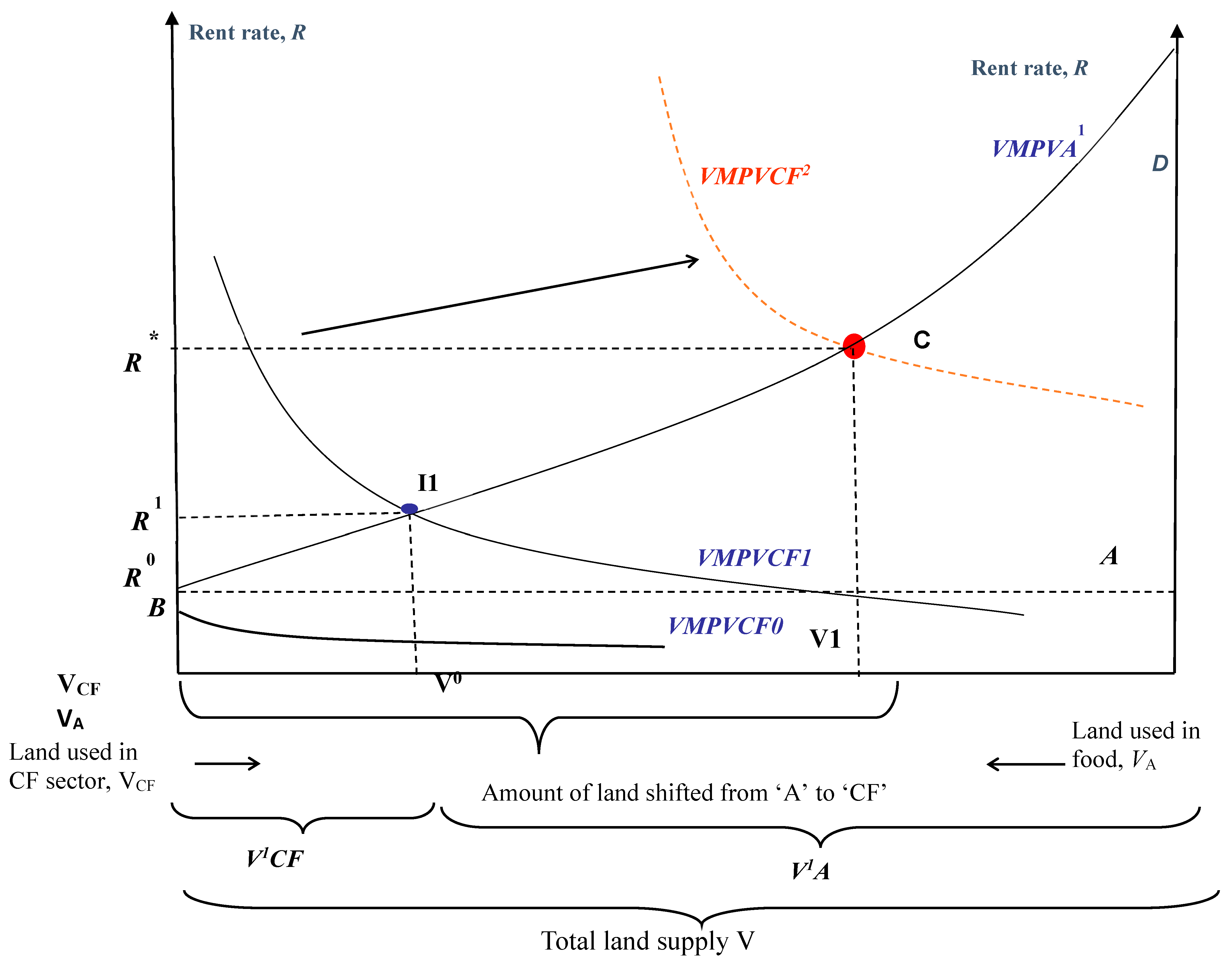
In the model that follows, we consider a small open economy and its ‘structural change’ in terms of the evolution or disappearance of a sector in response to external stimuli causing changes in production. The crops and livestock trade data include cash crops. First, we consider the agriculture (A) and manufacturing (M) (composite nonagricultural) sectors. The CF sector (C) requires land. The entry of CF brings about a structural change within the agricultural sector. Some land moves from the traditional food-producing agricultural sector to nonfood cash crops that it exports entirely. Unlike the typical model of interindustry trade (Heckscher-Ohlin and its variants), what we consider here is the complete elimination or vanishing of a sector and/or the emergence of a new sector (i.e., contract farming) at the expense of the existing ones. CF, therefore, brings in a discrete change in the output baskets as a new separate sector splits out. Theoretically, the situation resembles problems analyzed by a class of models called the “finite change” models. New traded sectors appear and disappear due to changes in competitive forces brought about by policy intervention. In the model, a new equilibrium is qualitatively different from the prechange situation (Beladi et al. 2013; Marjit et al. 2007, 2013; Marjit and Mandal 2015; Das 2013, 2018; Jones 2014, 2018; Marjit 1990).
Notations to describe the model structure are:
Pj: Exogenously given prices for jth final good output, ∀j ∈ {XM, XA, XC}.
XM: Import-competing manufacturing sector.
XA: Agricultural sector.
XC: Contract farming sector.
W: Labor’s wage.
r: Return to capital (generic).
V: Intersectorally mobile land (in general) in broader terms of the agriculture sector.
VF: Land under CF (i.e., acquisition of land under deal irrespective of modes of acquirement).
VA: Land for agriculture.
R: Return to V (generic land types).
a i j = ith input required to produce 1 unit of the jth final good, i = K, L, V.
d a i j a i j = t ( t > 0 ) is the uniform rate of technical progress. A negative sign indicates that unit factor requirement shrinks thanks to boons of technological advancement.
θ i j = w a l j / P j is the distributive share of lth labor-types in j ∈ {XM, XA, XC}, ∀l.
θ k j = r k j a k j / P j is the distributive share of the owner of specific capital K for j = C, M.
θ v j = R j a v j / P j is the distributive share of the owner of Vth specific land for j ∈ {A, F},∀v∈{VF, VA}.
λ i j = a i j Y j / f j is jth commodity’s input share in ith factor’s endowment, where Y is generic output and f is generic endowment.
“∧“ = proportional changes for a variable, say x, such that x ^ = d x x .
The production structure of the economy before the entry of CF is as follows:
X M = X M ( L , K ) ; X A = X A ( L , V )
L (labor), K (capital) and V (land) are the factors of production, and this is a specific factor model (see Feenstra (2003), chapter 3). The entry of CF in the above economy is depicted in Figure 3.
Without CF, the value of marginal productivity of land (VMPVA) curve for A is the only curve in the land market. If full land employment is assumed, then R0 is determined when the land market is cleared. Suppose for some reason (due to higher cost or bad technology and lower price) that rent (marginal value productivity of land (VMPVCF)) in CF is even lower than that in agriculture (VMPVA). It must imply that it would be much lower than that in the agriculture subsector with no land in CF (i.e., without CF). Then, all land is allotted to the ‘A’ sector (i.e., case of complete specialization). See Figure 3, where VMPVCF is much below VMPVA.
Whether CF can enter the agricultural sector or not depends on the CF sector’s VMPV (VMPVCF) position: it can join if it can pay at least R0. If VMPVCF shifts left up to intersect VMPVA at higher equilibrium at I1, we could see that land allocation does not start until the ‘gap’ between these two VMPV curves shrink. In I1, the land going to the CF sector is much less (V0VCF), with the scope of productivity benefits being less. However, suppose VMPVCF shifts a ‘big way’ upwards (thanks to much higher world price or superior technological progress with prospects of cost-reduction). The new point of intersection is at new equilibrium C. In that case, it will be lucrative to switch land from the “A-sector” to CF. Thus, any VMPV curve uniformly below R0 (say, at VMPVCF0) implies that entry is impossible. In other words, the position of VMPVCF depends on two scenarios: Firstly, given prices, an entrant must have a sufficiently good technology (MPV) for land usage. Secondly, on the other hand, given technology, international prices decide entry. As any of these scenarios happens, it increases the probability of entry as the VMPV curve for CF shifts to the right (VMPVCF2). This makes agricultural products—such as cash crops—better candidates for CF, at least for some landowners. Once CF enters, allocation of land depends on the relative position of the VMPV curves. From Figure 3, we observe:
(1)
New R = R* is higher than the pre-CF returns to land (say, R0).
(2)
‘V1V’CF amount of land moves from the agriculture to the CF sector with much higher VMPVCF.
(3)
Value of output in the traditional agricultural sector changes from DVVCFA to DVV1C.
(4)
Total value of agricultural products increases from DVVCFA to DVV1C + CV1VCFB, out of which the latter is exported.
Choice of production technique in keeping with endowment ratio will determine the full-employment production bundles (see Sen 1968). See Figure 4. Cases such as CF become labor-intensive (i.e., factor intensity reversal) and will alter the consequences, although similar logic prevails. We ruled out that case because the basic premise is that CF ushers in better technology or benefits in the sector.
The isoquants for each sector are the unit-value isoquants. For any given R/W ratio, CF-production has a higher land–labor ratio than the A sector and vice versa. Here, if the economy incompletely specializes in both the A and CF sectors, then it must be the situation that makes it so that the costs of producing one-dollar worth of both of them must be the same. This is possible if the minimum cost of production for XA and XC both lie on the same isocost line, whose slope is–R/w. Two rays from the origin form the ‘cone of diversification.’ Thus, the condition that both ‘food’ crops and contract farming outputs are produced at full employment is that the relative endowment of labor vis-à-vis land must not exceed (or falls short of) the land–labor (or labor–land) intensity of both ‘A’ and ‘CF.’ (Caves et al. 2010).
To summarize, the possible ‘rise in price’ in the world market due to the scope of international trade provides the ‘positive’ incentives for shifting land from the food to an activity that could boost productivity (via access to better agricultural inputs). This causes the potential endogenous collapse of the traditional food sector (‘finite change’) and the emergence of a CF sector with output XC. The introduction of a separate sector, producing a distinct set of homogenous goods, but nested within the A-sector, is equivalent to splitting the ‘broad generic’ agriculture into two different sectors: producing, say, food (as before) and the other, say, cash crops. Such CF activities in the farming sector introduce new technology in selected tracks of land (in terms of different unit factor requirements). Let us suppose that the payment for this technology transfer accrues to its (foreign) introducers in terms of a fixed margin of unit prices, Where ρ < 1 is the proportion of unit prices accruing to the domestic economy and (1 − ρ) is the proportion of unit prices that is repatriated. We can then write:
Lemma 1. 
CF will be feasible if only if ρPC > PA P C > ( 1 / ρ ) P A   where   ( 1 ρ ) > 1 .
Necessary: Suppose total factor income (wl + rK + RV) before and after the introduction of CF is, respectively, Ω0 and Ω*. With zero profits, ρPC > PA implies Ω0 < Ω*, implying that the non-CF equilibrium becomes suboptimal as soon as CF opens up.
Sufficiency: A sufficient condition for CF to occur is that at least one factor of production can gain due to CF. If ρPC > PA, then the mobile factor (land) will obtain a higher return in CF than in the A sector. Therefore, landowners will be incentivized to reallocate land to CF, giving the endogenous production structure modeled below. Essentially, this transforms the above 2 × 3 specific factor model in Equation (1) to a 3 × 3 mixed specific factor Heckscher-Ohlin model: (agricultural and CF sectors are HOV production technology, and manufacturing is specific factor technology). Thus, the model becomes:
a V A X A + a V C X C = V
a K M X M = K
a L A X A + a L M X M + a L C X C = L
a V A R + a L A w = P A
a K M r + a L M w = P M
a V C R + a L C w = ρ P C
a i j = a i j ( R , r , w )
These are six independent equations in six variables: the three-factor prices and the three outputs. Note that the system is now decomposable into (2) to (4) and (5) to (7), where the three latter equations determine the factor prices. Unlike the previous model, now there are two mobile factors, labor and land (with restricted mobility between the two subsectors under agriculture).

4. Consequences of a Growing CF Sector

What are the consequences of CF in this small open economy? The simplest way to understand this is to make the sector grow and see what happens. Following the motivation of introducing CF in Figure 3, we consider two types of exogenous ‘shocks’: (i) changes in world prices of tradeable sectors; (ii) technical progress causing total factor productivity or factor-augmenting changes. In terms of Figure 3, both these changes lead to further shifts in the VMPV curves and are captured by the following equations of change:
θ L A w ^ + θ V A R ^ = P A ^
θ L C w ^ + θ V C R ^ = P C ^
θ L M w ^ + θ K M r ^ = P M ^
And the following equations of change for technology changes:
θ L A w ^ + θ V A R ^ = α
θ L C w ^ + θ V C R ^ = β
θ L M w ^ + θ K M r ^ = γ
The following two propositions immediately follow from the ‘magnification effects’ (see the Appendix A):
Proposition 1. 
If price of manufacturing and traditional agriculture remain constant then, X A ^ < 0 , X C ^ > 0 , X M ^ > 0  and  R ^ > r ^ > 0 > w ^ .
Proposition 2. 
R ^ > 0   i f f   α θ L C < β θ L A , and  w ^ < 0   i f f   β θ V A > α θ V C , r ^ > w ^   i f f   γ > w ^ ( a s   θ K M > 0 )  and  R ^ w ^ = α β θ   > 0   i f f   α < β .
Thus, assuming CF to be less labor intensive than the traditional agricultural sector, progression of CF in this economy (either through a further increase in its international price or improvement in its technology) predictably results in the shrinking of traditional agriculture and expansion of the CF and manufacturing sector. The extent of land switching and compositional changes in the product mix of XA and XC is contingent on the interplay of elasticity of substitution between demand and supply (see Appendix D). Further, laborers lose while other factors of production gain. If labor income is lower than the income of capitalists and landowners, income inequality increases. The only way rising income inequality can be reversed is through improvement in technology in agriculture (via Proposition 2). The key insights from these two lemmas imply that given no change in the world market, if demand for nonfood crop expands, it is lucrative to produce more of that CF-good at the expense of other sectors suffering from contraction. However, that might be short-run myopia; in long-run, other concerns surface up, such as employment, welfare, and food shortages.
Further we have:
Proposition 3. 
Contract farming increases GDP.
Let ρ Pc = Pc* (the price the local producers receive) and GDP (Ω) is evaluated at Pc* (around the neighborhood of change in it). By the envelope theorem, /dPc* = Xc(PC) >0. This comes via a rise in VMP of land thanks to an increase in Pc or technology. Additionally, note that “µΩ” is spent on food. Therefore, µΩ = PADA (the demand for XA). We choose M as the numeraire good (PM = 1) so that GDP is in the units of M and PADA is in the units of M. Obviously, expansion of nonfood production as well as cash crops will raise production as a whole and will positively affect GDP from the production side.
Generally, it follows when P A ^ = 0 , d Ω Ω = P c X c Ω ( X C ^ + P C ^ ) .
Now,
d Ω / dPc * = Xc   d Ω Ω = d P c · X c Ω = d P c P c · P c X c Ω = P c ^ · θ C Ω Ω ^ = P c ^ · θ C Ω
Equation (15) implies that percentage change in GDP is directly proportional to price rise in the CF-sector and share of CF in the GDP ( P c X c Ω = θ C Ω ) with a positive slope (QED).

5. Food Security, Inequality, and Contract Farming

5.1. Balance of Trade and Food Imports

We assume that the traditional agricultural sector is the import sector. To sustain the pre-CF equilibrium, the manufacturing sector is the export sector. For further simplicity, let us assume that the entire manufacturing output is exported. Without CF, export earnings are PMXM and import is PADAPAXA = PA (DAXA), where DA is the domestic demand for food. Of course, relative budget shares of the outputs will determine the extent of net welfare impacts. In this case, household income and wealth effects and Engel aggregation conditions need to be satisfied.
Let T be the balance of trade:
T = PMXMPA (DAXA)
If we further assume homothetic preferences and that a constant proportion 0 < µ ≤ 1 of income goes to domestic demand for food, then
PADA = µ (w* L + r* K + R* V) = µY
where Y is GDP at factor cost (income), w* L + r* K + R* V.
However, GDP from the production side is:
Ω = P A X A + P M X M + P C X C
GDP from the income side or value-added and GDP at factor cost must match, and one is dual to the other and vice versa (Feenstra 2003). We assume GDP and GNP differences accounted for via net factor income from abroad are already incorporated via trade balance condition.
Using duality theory, we know Y = Ω so that we can use it interchangeably. If the entire amount of manufacturing output is to be exported, people only consume food, so that µ = 1. A representation of the pre-CF situation by a ‘0’ and post-CF situation by a ‘*’ trade surplus (pre-CF) is:
T0 = PMXMPA (DAXA). when μ = 1
With CF, on the other hand, export (earnings) changes to (1 − ρ) PCXC + PMXM and import (earnings) remains at PADAPAXA. Balanced trade (using (17)) then implies (0 < μ < 1):
T * = [ ρ P c X c + P M X M ] [ P A D A P A X A ] = [ ρ P c X c + P M X M ] [ μ Ω P A X A ]
Proposition 4. 
Introduction of CF increases food import and creates a trade surplus.
Proof. 
Given exogenous price of food, food import will increase if (D0AX0A) < (D*AX*A). □
Note that we have already shown that GDP increases (before). This will increase DA. By Proposition 1, XA falls. Thus, the above inequality is always true.
Now,
µ · d Ω / dPc * = d ( P A D A ) / dP C * ·   d T * d P c * = X c μ X c
Thus, trade surplus (T*) goes up by XC (1 − µ) (note that the change in XA has been accounted for by the envelope condition). Thus, we must have a trade surplus. Since exports will always pay for our imports, we increase food imports. Therefore, technically countries can import food to mitigate demand. There is nothing in the model to show that food production goes to zero (see Section 2 for exposition to cone of diversification). Hence, food imports might inflate but CF might contribute to a trade surplus with possibilities of food shortages, to which we turn in the next section.

5.2. The Short-Run Consequences of CF

Suppose there are ‘n’ such countries that are exactly similar (homogeneous) and symmetric. Each one engages in CF so that land devoted to food is slashed. Taken together, they represent a considerably large chunk of the world food market, and no one can refrain from engaging in CF. Thus, there will be an adverse supply shock—causing a left upward shift of the world food supply. For less developed countries (LDCs), more of the rising income (relaxing the initial budget constraint) is spent on food (without Engel’s law setting, in which Engel’s law states that proportion of income spent on food consumption falls although absolute expenditure on food rises with income). Income elasticity of demand for food is positive and less than unity. With similar sizes, internalization is possible in the long run unlike heterogeneous size countries where some countries might not cooperate to stop or regulate CF.
Due to CF, as GDP rises, demand is escalated. Thus, overall, it has a price effect via escalating demand (causing the demand curve for food to shift rightward). In any event, the adverse supply triggers food inflation as food prices rise. This is a high price externality due to excessive CF. Thus, import food prices might increase if many small countries pursue CF (i.e., the aggregate has a price effect).
World demand = D W A = i = 1 n P i A D i A and world supply = S W A = i = 1 n S i A .
In the case of heterogeneous sizes (nonsymmetric), D i A = μ i A ( Y i ) · Y   i . Suppose such small open economies are heterogeneous in terms of their size where P i A D i A = μ i A Y i , S i A = P i A X i A . World equilibrium for the food sector (XA) is given by:
D W A = S W A i μ i A Y i = i P i A X i A
In the post-CF case, for each small economy, GDP (Yi) rises and XA shrinks. Thus, i μ i A Y i > i P i A X i A causing PA to rise in general and for each ‘i = 1, 2, …, n. See Figure 5a,b below.
As world food prices shift up and demand remains the same (or even rises), some economies quit CF, and supply responds until the price comes back to the previous level. On top is Engel’s law, causing food prices to inflate more, creating a self-correcting mechanism such that CF receives less and less land, causing the limited amount of land to be transferred from the agriculture (food-crop) sector. Given a fixed amount of nonrenewable scarce land to be ‘divided’ between CF and non-CF sector, land-conversion between two competing uses are important, as physical shares of land used in CF vis-à-vis the food sector must satisfy land-constraints without expansion of land via deforestation or fallow land being ‘recycled’ into use. Elasticity of land conversion (switching) could be an important factor for the extent of CF vis-à-vis non-CF, as that depends on relative returns in those activities.
Thus, in the short run, with the symmetric n-country price-taking model due to the fallacy of composition, the aggregate price effect is not internalized by each country, and there is excessive CF in each small country. Internalization of the international price rise occurs in our model via movement of firms from CF to food sector triggered by price hike thanks to the combined effect of adverse supply and favorable demand impact (Figure 5a) in the long run. As land moves to CF, the world supply of food (Sw) shifts left and up thanks to a slash of land in the traditional agricultural sector for food. Food prices inflate due to a leftward supply shift with the same or more demand, causing two rounds of price increases. As real wage falls (in terms of food prices -w/PA), workers lose unambiguously, resulting in insecurity (relative poverty increases with the rise in inequality as real returns to workers fall). This causes loss of welfare initially without internalizing the externality due to high price. This price rise is a binding constraint with a vertical supply curve (inelastic) in Figure 3b. In this case, we think of a global social planner who will allocate a smaller proportion of land to CF in countries with higher GDP (Y) and less to CF if the world demand curve is highly inelastic. Suppose i μ i A Y i = i P i A X i A and PA are fixed. As XA falls but μ i A Y i  rises, PA has to rise. Post-CF supply (vertical) shifts further left, and PA rises with the same or more demand. If this is ‘internalized,’ then in the long run, “Sw” shifts right, and with increasing marginal cost, the Sw curve becomes more elastic but does not go back to the ‘old’ level. XA rises, and PA falls but not entirely. The main question is that the long-run adjustment may take a very long time depending on the nature of contracts and regulations, management, and laws about CF, etc. Thus, the vertical supply curve may keep on shifting left and not move back due to the long-run process.
Proposition 5. 
In the short run, uncoordinated international expansion of CF will increase international price of food. In the long run, there is an endogenous limit to CF.
As a result, food-importing countries will suffer (a) a decline in their terms of trade and (b) the Engel’s law will aggravate depravation in less developed countries in the short run. International coordination of proportion of land allocated to nonfood producing CF is necessary to address this issue.
Thus, the general equilibrium model developed above provides a framework for analyzing the contentious issues of contract farming. So far, no general equilibrium model has been developed in the line of mixed specific factor and finite change type in this context. As has been mentioned in Section 1 and Section 2, development economics literature has these kinds of models for the formal–informal sector or Harris–Todaro Model (see Marjit and Acharya 2003; Marjit and Kar 2019). However, except for Das (2013, 2018) in the land-acquisition context, this kind of model has not been used for researching CF versus agriculture trade-off. This model is entirely different in flavor, as it has the novelty of using structural change in the macroeconomy via finite change aspect, and hence, the results are distinguishable from previous studies.

5.3. The Growth–Inequality Trade-Off of Contract Farming: Numerical Simulations

One of the main implications of introducing CF in the above model is the possibility of a simultaneous rise in GDP and a rise in inequality captured by the rental-wage ratios. What does it mean for the social welfare (S) of the country? In particular, does targeting social welfare put a limit to the expansion of CF in a country? Let us assume a simple S- function of the form:
S = α Ω ( 1 α ) R w
S is social welfare, α is the weight attributed to GDP ( Ω ) , and R w is the proxy for inequality in the country.
From (9) and (10), via Cramer’s rule (see Appendix B): R w ^ = 1 θ P C P A ^ which yields, via integration, the following (as generically, ( x ^ = d ln x ):
ln R w = 1 θ ln P C P A + ln c 1 , where ‘ln C1’ is the integration constant. On further simplification, we get:
ln R w = ln P C P A 1 θ + ln c 1 = ln c 1 P C P A 1 θ R w = c 1 P C P A 1 θ
Additionally, from (18) above, Ω ^ = P c ^ · θ C Ω , ensuring positive relationship, which gives, via integration,
GDP = Ω = c 4 · P c θ C Ω ( C 4   is   constant )
From (43), further we can write, given L ^ = V ^ = 0 , P A ^ = 0 = X A ^
X C ^ X A ^ = σ S [ P C ^ P A ^ ] must hold.
Assuming X A ^ =0, we have d l n X C = σ s · d l n P C P A
Via integration of both sides, we get:
l n X c = σ s · l n P C P A l n c 5 , where lnC5 is constant of integration.
Simplifying,
X c = c 5 · P C P A σ S
Ω = Λ + c 5 · P C P A σ S + 1   w h e r e   Λ = P A X A + P M X M
Putting (21) and (24) in (20), we have:
S = α Λ + c 5 · P C P A σ S + 1 ( 1 α ) c 1 P C P A 1 θ
An inspection of (25) shows that depending on the values of the parameters ( Λ , σ S , α , and θ ( θ V C θ V A = θ L A θ L C ), assuming the constants of integrations to be 1), the relationship between (welfare) and P C P A (price ratio) (a) is nonlinear and (b) can be negative, positive, or a mix of both.
Of particular interest are the parameter combinations that produce inverted U-shaped curves: the government in these cases has reason to restrict CF to check inequality even though the international terms of trade are favorable. Note that Λ determines the intercepts of the curves on the welfare axis (higher is the aggregate size of the non-CF sectors, higher is the pre-CF welfare level). The interplay between the other three parameters in the system can be summarized as follows (representative cases are reported in Figure 6a–c): (i) elasticity of substitution in supply between the goods produced by traditional agriculture and CF, (ii) the difference in cost-shares between the two goods, and (iii) the relative weight given to GDP has a positive impact on ‘S’. It is always possible to generate long monotonically increasing or decreasing segments in the relationship in Figure 6 by an appropriate set of parameters. Different combinations of α, θ, σ, and Λ are chosen to see how social welfare behaves with a constellation of values and their rise and fall. In Figure 6a, corresponding to (i) above, only “σs” is reduced from 1 to 0.5 to see that an inverted relationship occurs, supporting our explanations. In Figure 6b, we reduce ‘α’ to 0.4 from 0.6 in the case of Figure 6a, while others remain in the same range, and we get the same inverted U-shaped curve. Contrary to them, in Figure 6c, we raise values of ‘α’ and Λ ’, while ‘θ’ falls given ‘σ’, and we obtain a similar kind to Figure 6a. This means that GDP and social welfare depend on these four parameters and share of CF.
It is possible to make several observations about Equation (25) and the figures in Figure 6a,c. First, as we pointed out in the introduction, success of CF is context dependent. Additionally, we demonstrate that in a competitive economy, context-dependence is limited only to the issue of social welfare but not to its components (GDP and income inequality). Secondly, CF is unequivocally beneficial to a competitive economy, provided that the size of the non-CF agriculture (A) is sufficiently large. Thus, large economies such as India with a large and competitive agricultural sector should not hesitate to allow CF within their countries. The probability is high that they will contribute positively to social welfare. In a study, Seogo (2022) showed that in rural Burkina Faso, engaging in nonfarm activities could solve food insecurity, as nonfarm income contributes positively to food stability and expenditure on food.
Finally, the effect of terms of trade on social welfare demonstrated in this section reiterates the observations made in Section 5.2. The positive outcomes of CF (wherever they occur) will be reversed if a sufficiently large part of the land is allocated to nonfood contract farms in many countries, leading to the deterioration of terms of trade of the food importing country. A key message is that increasing allocation of land to nonfood cash crop would aggravate social and individual welfare for a food-importing nation and will deteriorate the terms-of-trade.
Thus, from the previous sections we see that the theoretical results derived from our model are quite strong in terms of explaining the phenomena of contract farming in the agriculture sector and its different impacts on welfare and returns to factor owners with different class interests. One of the salient features of our framework is ‘fallacy of composition’, by dint of which we have shown some counter-intuitive possibilities in terms of movements of relative supply and demand in the food market. In fact, linking food-insecurity issues to commercialization of agriculture is a novelty for policy implications as well, esp. for predominantly agricultural nations such as China, India, and Bangladesh on one hand, and Europe and North America on the other hand. Herein lies the efficacy of general equilibrium formulation that the past studies have not attempted. Hence, this framework has immense applicability for deriving policy simulations, as has been illustrated in our numerical exercise in the penultimate section.

6. Concluding Remarks and Policy Insights

CF is a contentious issue. Food insecurity is a grave concern. It is actively researched in the literature on FDI in agriculture and its impacts on smallholder agriculture. This research contributes to this debate by looking at the outcomes of this phenomenon in a competitive structure. Our main conclusion is that CF is pro-growth but anti equity. Further, since, by its very definition, CF solves the problem of any food deficiency in a country through food import financed by the export of the CF good, there is no scope for any concern on the possible deterioration of the trade balance. Since these results are not context-dependent and will happen in any competitive economy with some restrictions on the factor intensities of the CF and non-CF sectors, it contributes to clarifying the confusion on the overall desirability of CF.
The opposing effects of CF on growth and equity lead to a social dilemma. This dilemma can explain at least a part of the ongoing debate on the desirability of CF in recent times, especially in countries such as India. The debate becomes meaningful only when CF operates on a significant proportion of agricultural land for a predominately rural economy and to the relative size of the rest of the economy for more advanced economies. If CF is marginal relative to aggregate GDP, both economic and social welfare is guaranteed through CF, and governments might not regulate them. However, even in these economies, the fallacy of composition can create a reversal of gains from CF in the short run. If many countries pursue similar policies, world food shortage is inevitable, leading to falling terms of trade and welfare loss of a food-importing small open economy. In this case, the strategy of paying for imports through exports of the CF sector will not be sufficient to generate welfare advantages from CF. An apparent possibility of social welfare behaving in ways that are inimical to the country’s interest keeps the door of uncertainty open for government policies in this regard. A politico-economic dimension to the issue may help resolve this and other contentious issues. This paper attempts to figure out some context-neutral economic logic toward policy formation and offer policy insights for addressing the trade-off between food sufficiency and growth via adoption of contract farming. However, although this research focuses on formalizing the idea of contractual farming practices and derives important theoretical insights, the future direction of research should be (i) to do case studies in the context of developing countries such as India, China, and some African nations; (ii) empirically test the hypothesis derived from this research; (iii) check food insecurity and poverty aspects of such land-acquisition (given these limitations, our simulation is a step forward in that direction); and (iv) considering technical progress—such as biotechnology, green revolution-type technical change, etc.—could be a helpful extension for tracing the intersectoral spillover effects with positive externalities. These are beyond the scope of the current paper.

Author Contributions

All the authors contributed from the initial to final stages with considerable inputs. Conceptualization: G.D., S.M. and R.B.; methodology: S.M. and R.B.; Software: R.B. and G.D.; Validation: R.B.; Formal analysis: R.B., G.D. and S.M.; Investigation: R.B. and G.D.; Resources: R.B.; Data curation: R.B.; Writing—original draft preparation: G.D. and R.B.; writing—reviewing and editing: R.B. and G.D.; Supervision: S.M. All authors have read and agreed to the published version of the manuscript.

Funding

This research received no external funding.

Data Availability Statement

Not Applicable.

Acknowledgments

Authors acknowledge the useful comments from the participants in the Conference in Trade and Development, Indira Gandhi Institute of Development Research (IGIDR), Mumbai, India during December 2020. The authors are also thankful to the participants in the Econometric Society Asian Meeting, Malaysia, (Econometric Society Asia Chapter)) in June 2021, and seminar participants at the University of Tartu, Estonia in 2020, Indian Statistical Institute, New Delhi, Annual Conference in Development Economics, 2021. A different version of the paper was also presented at the American Economic Association ASSA-AEA Poster Session Meeting in January 2019, and International Economic Association (IEA) Meeting at Bali, Indonesia, in 2020-2021 via webinar. We thank five anonymous referees for their insightful comments, which were extremely helpful to revise the submitted draft.

Conflicts of Interest

The authors declare no conflict of interest.

Appendix A. Model Without Contract Farming

The general equilibrium structure is given by the following equations:
a V A X A = V
a K M X M = K
a L A X A + a L M X M = L
a V A R + a L A w = P A
a K M r + a L M w = P M
a i j = a i j ( R , r , w )
where the returns to land, capital, and labor are R, r, and w, respectively, and aij is the unit factor requirements. (A1) to (A5) are five independent equations in five variables, the three-factor returns, and the solved outputs. Being mobile, labor endowment is allocated by the equality of the value of marginal products of labor in the two sectors. Endowment differences will cause specialization in different sets of goods, and factor prices will diverge ex post.

Appendix B. Proof of Proposition 1

As Pc rises by more, there will be intersectoral migration of labor from the shrinking traditional agriculture sector to contract farming. Thus, X A ^ < 0 , X C ^ > 0 ,   and   X M ^ > 0 .
Now, using (9) to (11), we can write:
R ^ = P A ^ θ V A θ L A θ V A w ^   and   R ^ = P C ^ θ V C θ L C θ V C w ^ .
So R ^   and   w ^ are negatively related, definitely, so ‘R’ increases while ‘w’ falls. If CF is land- or capital-intensive, the extent of the rise in the former price ratio must increase ‘R’ and lower ‘w.’ Thus, when P C ^ > P A ^ > 0 , R ^ > w ^ .
If θ L A > θ L C (or, equivalently reasonably higher θ V C > θ V A ), due to the Stolper–Samuelson effect, ‘w’ might fall more and cause pronounced changes in ‘R’ (in the opposite direction). Similarly, r ^ = θ L M θ K M w ^ r ^ > 0   iff   w ^ < 0 .
However, in Section 2, CF entry happens only when P ^ C > P ^ A 0 . For a perfectly general case, let us write: P ^ C = δ + P ^ A , where ‘ γ ’ is kind of ‘mark-up’ over P ^ A so that even without any changes in PA, higher values mean P ^ C > 0, causing a shift to CF (and more repatriation of profit).
Then, using (9) and (10), we can write:
θ L A w ^ + θ V A R ^ = P A ^
θ L C w ^ + θ V C R ^ = P C ^ = P A ^ + δ
Cramer’s rule yields,
w ^ = P A ^ θ V C P C ^ θ V A θ L A θ V C θ L C θ V A = P A ^ θ V C ( δ + P A ^ ) θ V A θ = P A ^ δ θ V A θ = P C ^ δ θ V C θ
where θ = θ V C θ V A = θ L A θ L C .
Additionally,
R ^ = P C ^ θ L A P A ^ θ L C θ = P C ^ + δ θ L C θ = P A ^ + δ θ L A θ
so that,
R ^ w ^ = P C ^ P A ^ θ = δ θ > 0 R ^ > w ^   as   δ θ ( by   assumption ) .
From (A9), w ^ = P C ^ δ θ V C θ = P C ^ [ 1 δ θ V C P C ^ ( θ V C θ V A ) ] .
As δ > 1 , θ V C ( θ V C θ V A ) > 1 , δ θ V C ( θ V C θ V A ) > 1 , so w ^ 0 ,   iff   1 δ θ V C P C ^ ( θ V C θ V A ) P C ^ > 1 . That means that if PC rises (relative to PA) and is exceptionally high, it will lower ‘w’.
From (A9), we can prove that w ^ < 0   iff   1 > P A ^ 0 ; that is, even if PA inflates but at a much lower rate than PC, clearly from (A9) and (A10), if P C ^ > P A ^ 0 , then R ^ > P C ^ > P A ^ , R ^ > 0 , w ^ < 0 . It is obvious that ‘R’ rises and ‘w’ falls depending on  δ   and   θ .

Appendix C. Proof of Proposition 2

Note that change in labor demand within the agricultural sector via CF is:
L d ^ = λ L A a L A ^ + λ L A X A ^ + λ L C a L C ^ + λ L C X C ^
where λ L i = a L i X i L , and a ‘^’ over a variable implies relative change due to the entry of CF.
Given factor prices ‘w’ and ‘R’, a L A ^ = 0 . Our assumption regarding labor-saving technology in CF implies that a L C ^ < 0 . On the other hand, with ‘R’, fixed land allocation between agriculture and CF sectors are fixed, and so are unit land requirements; hence, land allocation is given by:
V ^ = 0 = λ V A a V A ^ + λ V A X A ^ + λ V C a V C ^ + λ V C X C ^
With a V A ^ , a V c ^ = 0 (as ‘w’ and ‘R’ are fixed); thus:
X C ^ = λ V A λ V C X A ^
Putting (A13) in (A12), λ L A λ V C λ L C λ V A λ V C X A ^ +   λ L C a L C ^ = L d ^
Since a L C ^ < 0 so that λ L C < 0 , a sufficient condition for L d ^ < 0 is the term in the first bracket in the above equation, which is less than zero.
Ex post with CF, as the land moves from XA, CF (XC) will have higher cost-shares of land, implying  θ = θ V A θ V C = θ L C θ L A < 0 .
Also, R ^ = α θ L C β θ L A θ V A θ L C θ V C θ L A > 0   iff   α θ L C < β θ L A ( g i v e n θ < 0 ) .
This implies also α β < 1   as   θ L A > θ L C .
Similarly, for w ^ < 0   iff   β θ V A α θ V C > 0 β θ V A > α θ V C ( g i v e n θ < 0 ) .
As above, we can prove that it holds when α β < 1   as   β θ V A > α θ V C ,   expost   θ V C > θ V A
Hence, we can infer that: R ^ w ^ = α β θ   > 0   iff α < β .
From (A13), r ^ = γ θ L M w ^ θ K M r ^ w ^ = γ w ^ θ K M ( as   θ L M + θ K M = 1 ) .
As w ^ < 0 ,   and   γ > 0 ( γ w ^ ) > 0 . Additionally, with technical progress in the manufacturing sector, the fall in wage rate must be superseded by the increase in the marginal productivity of capital. It is quite intuitive that contingent on a higher rate of technical progress and accrual of its spillover benefits in the CF sector, there is a maximum return to the factor used in the CF sector, which survives as the allocation of land enables more earning landowners to undertake CF-mode.

Appendix D. Proof of Proposition 5

Following Jones (1965, 1971), we can write that:
X A ^ = θ L A σ A ( w ^ R ^ )   and   X C ^ = θ L C σ C ( w ^ R ^ ) X A ^ > X C ^   iff   θ L A σ A > θ L C σ C θ L A / θ L C > σ C / σ A
However, as XA is relatively more labor-intensive than XC (see Section 3 and Section 4 above), θ L A > θ L C θ L A θ L C > 1 σ A > σ C , where σ A , σ C  are the elasticity of substitution between labor and land in the respective sectors. Using endowment shares, we derive (see Appendix B) that:
X C ^ = λ V A λ V C X A ^
Using envelope conditions, V ^ = λ V A X A ^ + λ V C X C ^ .
Further combining these, we get X A ^ > 0   iff   λ L A λ V C > λ L C λ V A λ L A > λ V A .
As we know, V A + V C = V ¯ , we write, a V A X A = V A   and   a V C X C = V C   or ,   V C = ( 1 ω ) V , 0 < ω < 1 .
Let R A R C F . Then, ω determines the extent of land switching ex post the rise in world food prices (as explained before). However, such switching or conversion will depend on the elasticity of substitution between XA and XC on the supply side, and hence on relative factor price changes (see Jones 1965).
Following Jones (1965, 1971), we can further derive and write (more in the Appendix later):
X A ^ X C ^ = 1 λ ( L ^ V ^ ) + σ S [ P A ^ P C ^ ] = 1 λ σ D σ S + σ D ( L ^ V ^ )
where σ S is the elasticity of substitution (supply side) between food crops and CF output, and σ D is the elasticity on the demand side triggered by  P A ^ / P C ^ . Thus, land-switching and compositional changes in the product mix of XA and XC are contingent on the interplay of demand and supply captured by σ S and σ D . Additionally, we can derive:
w ^ r ^ = 1 θ L M ( P M ^ r ^ ) w ^ R ^ = 1 θ L A ( P A ^ R ^ ) w ^ R ^ = 1 θ L C ( P C ^ R ^ ) σ A = a L A ^ a V A ^ w ^ R ^ σ C = a L C ^ a V C ^ w ^ R ^
Using the above block of equations, we infer: 1 θ L A ( P A ^ R ^ ) = 1 θ L C ( P C ^ R ^ ) , and hence, P A ^ > P C ^   θ L A > θ L C . As long as labor-demand increases with land shifting from CF to the food sector, Dw moves right ( w ^ > 0 ). Using the previous relationship, a la Jones (1965), we get:
σ A > σ C a L A ^ a V A ^ >   a L C ^ a V C ^ a L A a V A ^ > a L C a V C ^
and, as before, σ A > σ C   λ L A > λ V A .
Combining all these conditions, we can argue that, given endowment shares such that λ L A > λ V A  and cost-shares such that θ L A > θ L C , price changes like P A ^ > P C ^ —triggered by excessive CF shifting Sw leftward and Dw remaining the same or shifting right (due to increase in GDP)—will induce an endogenous limit on CF via elasticity of substitution in production (between L and V)—see Figure 5a,b. Thus, it will ensure that X A ^ > X C ^ .

Notes

1
The paper explores the effect of introducing a CF sector in the existing agricultural sector of the economy; hence, it is initially assumed that the cash crop-producing CF sector is not remunerative at the current international price of cash crops. The introduction of such a CF sector leads to an increase in inequality—on which there is more to come in the subsequent Section 4 and Section 5. This has been highlighted in the paper. We thank an anonymous referee for extremely useful comments on clarification.
2
Note that Hicks’ neutral technical progress is considered in the paper, so technical progress is not ignored. It should further be noted that whether technological improvement is beneficial to the economy depends on where the technological improvement occurs. Additionally, economies of scale is extremely important. However, it is outside the scope of the paper, as it assumes perfectly competitive markets. A similar analysis in the context of an oligopolistic or a monopolistically competitive agricultural market can address this issue.
3
This is an important area of future research, as this type of effect will both increase GDP as well as improve inequality. The effect of cost advantages is a complex issue even in this context of a small open competitive economy. Hence, it is not considered here. This is beyond the scope of this paper due to parsimony and is the subject matter of another paper.

References

  1. Andriamparany, Jessica Noromalala, Hendrik Hänke, and Eva Schlecht. 2021. Food security and food quality among vanilla farmers in Madagascar: The role of contract farming and livestock keeping. Food Security 13: 981–1012. [Google Scholar] [CrossRef]
  2. Barrett, Christopher, B. Maren, E. Bachke, Marc F. Bellemare, Hope. C. Michelson, Sudha Narayanan, and Thomas F. Walker. 2012. Smallholder participation in Contract Farming: Evidence from Five Countries. World Development 40: 715–30. [Google Scholar] [CrossRef]
  3. Baruah, Sampriti, Samarendu Mohanty, and Agnes C. Rola. 2022. Small Farmers Large Field (SFLF): A synchronized collective action model for improving the livelihood of small farmers in India. Food Security 14: 323–36. [Google Scholar] [CrossRef]
  4. Beladi, Hamid, Sugata Marjit, and Saibal Kar. 2013. Emigration, Finite Changes and Wage Inequality. Economics and Politics 25: 61–71. [Google Scholar] [CrossRef]
  5. Bellemare, Marc F., and Sunghun Lim. 2018. In all shapes and colors: Varieties of Contract Farming. Applied Economic Perspectives and Policy 40: 379–401. [Google Scholar] [CrossRef]
  6. Bjornlund, Vibeke, Henning Bjornlund, and Andre van Rooyen. 2022. Why food insecurity persists in sub-Saharan Africa: A review of existing evidence. Food Security 14: 845–64. [Google Scholar] [CrossRef] [PubMed]
  7. Campenhout, Bjorn van, Karl Pauw, and Nicholas Minot. 2018. The impact of food price shocks in Uganda: First-order effects versus general-equilibrium consequences. European Review of Agricultural Economics 45: 783–807. [Google Scholar] [CrossRef]
  8. Casaburi, Lorenzo, Michael Kremer, and Sendhil Mulainathan. 2016. African Successes Vol IV. Edited by Sebastian Edwards, Simon Johnson and David Weil. Chicago: NBER Book University of Chicago Press. [Google Scholar]
  9. Caves, Richard E., Jeffrey Frankel, and Ronald Winthrop Jones. 2010. World Trade and Payments: An Introduction, 10th ed. Pearson: Addison-Wesley. [Google Scholar]
  10. Chang, Ching-Cheng, Chi-Chung Chen, Min-Ching Chin, and Wei-Chun Tseng. 2006. Is Contract Farming More Profitable and Efficient Than Non-Contract Farming—A Survey Study of Rice Farms in Taiwan. Available online: https://econpapers.repec.org/paper/agsaaea06/21374.htm (accessed on 12 August 2019).
  11. Chen, Jiguang, and Ying-Ju Chen. 2021. The Impact of Contract Farming on Agricultural Product Supply in Developing Economies. Production and Operations Management 30: 2395–419. [Google Scholar] [CrossRef]
  12. Collier, Paul, and Anthony J. Venables. 2012. Land Deals in Africa: Pioneers and Speculators. Journal of Globalization and Development 3: 1–22. [Google Scholar] [CrossRef]
  13. Das, Gouranga G. 2013. “Moving” land across borders: Spatial shifts in land demand and immiserizing effects. Journal of Economic Policy Reform 16: 46–67. [Google Scholar] [CrossRef]
  14. Das, Gouranga G. 2018. Land-Grab in the presence of Skill formation. Book Chapter in Essays in Honour of Deepak Nayyar. In Economic Theory and Policy amidst Global Discontent. Edited by Ananya Ghosh Dastidar, Rajiv Malhotra and Vivek Suneja. London: Routledge. [Google Scholar]
  15. De Schutter, Olivier. 2017. The political economy of food systems reform. European Review of Agricultural Economics 44: 705–31. [Google Scholar] [CrossRef]
  16. Deininger, Klaus, and Fang Xia. 2016. Quantifying Spill Over Effects from Large Land-based Investment: The Case of Mozambique. World Development 87: 227–41. [Google Scholar] [CrossRef]
  17. Feenstra, Robert. 2003. Advanced International Trade. Princeton: Princeton University Press. [Google Scholar]
  18. Food and Agricultural Organization (FAO), Charles Eaton, and Andrew W. Shepherd. 2001. Contract Farming: Partnerships for Growth. Available online: https://www.fao.org/3/y0937e/y0937e00.htm#toc (accessed on 14 March 2017).
  19. Giller, Ken E., Thomas Delaune, João Vasco Silva, Katrien Descheemaeker, Gerrie van de Ven, Antonius G. T. Schut, Mark van Wijk, James Hammond, Zvi Hochman, Godfrey Taulya, and et al. 2021. The future of farming: Who will produce our food? Food Security 13: 1073–99. [Google Scholar] [CrossRef]
  20. Grossman, Sanford J., and Oliver Hart. 1983. Implicit contracts under asymmetric information. The Quarterly Journal of Economics 98: 123–56. [Google Scholar] [CrossRef]
  21. Gulati, Ashok, Devesh Kapur, and Marshall M. Bouton. 2020. Reforming Indian Agriculture. Economic and Political Weekly 55: 1–24. [Google Scholar]
  22. Hennessy, David A. 1996. Information asymmetry as a reason for food industry vertical integration. American Journal of Agricultural Economics 78: 1034–43. [Google Scholar] [CrossRef]
  23. Hoang, Viet, and Vinh Nguyen. 2023. Determinants of small farmers’ participation in contract farming in developing countries: A study in Vietnam. Agribusiness An International Journal. [Google Scholar] [CrossRef]
  24. Jampel Dell’Angelo, Grettel Navas, Marga Witteman, Giacomo D’Alisa, Arnim Scheidel, and Leah Temper. 2021. Commons grabbing and agribusiness: Violence, resistance and social mobilization. Ecological Economics 184: 1–13. [Google Scholar]
  25. Jones, Ronald Winthrop. 1965. The Structure of Simple General Equilibrium Models. Journal of Political Economy 73: 557–72. [Google Scholar] [CrossRef]
  26. Jones, Ronald Winthrop. 1971. A Three-Factor Model in Theory, Trade and History. In Trade, Balance of Payments and Growth. Ch. 1. Edited by Bhagwati, Jones, Mundell and Vanek. Amsterdam: North-Holland. [Google Scholar]
  27. Jones, Ronald Winthrop. 2014. Heckscher–Ohlin and specific-factors trade models for finite changes: How different are they? International Review of Economics & Finance 29: 650–59. [Google Scholar]
  28. Jones, Ronald Winthrop. 2018. International Trade Theory and Competitive Models. Singapore: World Scientific. [Google Scholar]
  29. Krausmann, Fridolin, and E. Langthaler. 2019. Food regimes and their trade links: A socio-ecological perspective. Ecological Economics 160: 87–95. [Google Scholar] [CrossRef]
  30. Kushitor, Sandra Boatemaa, Scott Drimie, Rashieda Davids, Casey Delport, Corinna Hawkes, Tafadzwanashe Mabhaudhi, Mjabuliseni Ngidi, Rob Slotow, and Laura M. Pereira. 2022. The complex challenge of governing food systems: The case of South African food policy. Food Security 14: 883–96. [Google Scholar] [CrossRef]
  31. Little, Peter D., and Michael J. Watts. 1994. Living under Contract: Contract Farming and Agrarian Transformation in Sub-Saharan Africa. Madison: University of Wisconsin Press. [Google Scholar]
  32. Maertens, Miet, Bart Minten, and Johan Swinnen. 2012. Modern Food Supply Chains and Development: Evidence from Horticulture Export Sectors in Sub-Saharan Africa. Development Policy Review 30: 473–97. [Google Scholar] [CrossRef]
  33. Marjit, Sugata. 1990. A Simple Production Model in Trade and its Applications. Economics Letters 32: 257–60. [Google Scholar] [CrossRef]
  34. Marjit, Sugata, and Biswajit Mandal. 2015. Finite Change—Implications for Trade Theory, Policy and Development. In Development in India. Edited by S. Mahendra Dev and P.G. Babu. Berlin: Springer, (Indira Gandhi Institute of Development Research Silver Jubilee Volume). [Google Scholar]
  35. Marjit, Sugata, and Rajat Acharya. 2003. International Trade, Wage Inequality, and the Developing Economy. A General Equilibrium Approach. Physica-Verlag. Berlin: Springer. [Google Scholar]
  36. Marjit, Sugata, and Saibal Kar. 2019. International Capital Flows, Land Conversion and Wage Inequality in Poor Countries. Open Economies Review 30: 933–45. [Google Scholar] [CrossRef]
  37. Marjit, Sugata, Saibal Kar, and Hamid Beladi. 2007. Protectionary Bias in Agriculture: A pure Economic Argument. Ecological Economics 63: 160–164. [Google Scholar] [CrossRef]
  38. Marjit, Sugata, Saibal Kar, and Hamid Beladi. 2013. International Capital Flow, Vanishing Industries, and Two-sided Wage Inequality. Pacific Economic Review 18: 574–83. [Google Scholar] [CrossRef]
  39. Meemken, E. M., and M. F. Bellemare. 2020. Smallholder farmers and contract farming in developing countries. Proceedings of the National Academy of Sciences of the United States of America (PNAS) 117: 259–64. [Google Scholar] [CrossRef]
  40. Minot, Nicholas. 2009. Contract Farming in Developing Countries: Patterns, Impact, and Policy Implications. In Case Studies in Food Policy for Developing Countries, Domestic Policies for Markets, Production, and Environment. Edited by Per Pinstrup-Andersen and Fuzhi Cheng. Ithaca: Cornell University Press. [Google Scholar]
  41. Minot, Nicholas, and Loraine Ronchi. 2014. Contract Farming: Risks and Benefits of Partnership between Farmers and Firms. Viewpoint: Public Policy for the Private Sector No. 344. Washington, DC: World Bank. [Google Scholar]
  42. Mishra, Ashok K., Anthony N. Rezitis, and Mike G. Tsionas. 2020. Production under input endogeneity and farm-specific risk aversion: Evidence from contract farming and Bayesian method. European Review of Agricultural Economics 47: 591–618. [Google Scholar] [CrossRef]
  43. Nong, Yixin, Changbin Yin, Xiaoyan Yi, Jing Ren, and Chien Hsiaoping. 2021. Smallholder farmer preferences for diversifying farming with cover crops of sustainable farm management: A discrete choice experiment in Northwest China. Ecological Economics 186: 107060. [Google Scholar] [CrossRef]
  44. O’Hara, Sabine, and Etienne C. Toussaint. 2021. Food access in crisis: Food security and COVID-19. Ecological Economics 180: 106859. [Google Scholar] [CrossRef]
  45. Prowse, M. 2012. Contract Farming in Developing Countries: A Review. A savoir, Vol. 12. Paris: AFD, Agence française de développement. [Google Scholar]
  46. Robertson, Beth, and Per Pinstrup-Andersen. 2010. Global land acquisition: Neo-colonialism or development opportunity? Food Security 2: 271–83. [Google Scholar] [CrossRef]
  47. Rulli, Maria Cristina, and Paolo D’Odorico. 2014. Food appropriation through large scale land acquisitions. Environmental Research Letters 9: 1–2. [Google Scholar]
  48. Runsten, David. 1992. Transaction Costs in Mexican Fruit and Vegetable Contracting: Implications for Asociación en Participación. Paper presented at the XVIII International Congress pf the Latin American Studies Association, Atlanta, Georgia, March 10–12. [Google Scholar]
  49. Santangelo, Grazia D. 2018. The impact of FDI in land in agriculture in developing countries on host country food security. Journal of World Business 53: 75–84. [Google Scholar] [CrossRef]
  50. Sarkar, Abhirup. 2012. Development, Displacement, and Food Security: Land Acquisition in India. In Oxford Handbook of the Indian Economy. Edited by Chetan Ghate. Oxford: Oxford University Press. [Google Scholar]
  51. Sarkar, Swagato. 2014. Contract farming and McKinsey’s Plan for Transforming Agriculture into Agribusiness in West Bengal. Journal of South Asian Development 9: 235–51. [Google Scholar] [CrossRef]
  52. Schaffer, Harwood D., and Daryll E. Ray. 2020. Agricultural supply management and farm policy. Renewable Agriculture and Food Systems 35: 453–62. [Google Scholar] [CrossRef]
  53. Scoppola, Margherita. 2021. Globalization in agriculture and food: The role of multinational enterprises. European Review of Agricultural Economics 48: 741–84. [Google Scholar] [CrossRef]
  54. Sen, Amartya K. 1968. Choice of Techniques: An Aspect of the Theory of Planned Economic Development, 3rd ed. Oxford: Blackwell. [Google Scholar]
  55. Seogo, Windinkonte. 2022. Preventing households from food insecurity in rural Burkina Faso: Does nonfarm income matter? Agribusiness: An International Journal 38: 1032–47. [Google Scholar] [CrossRef]
  56. Swinnen, Johan F. M., and Miet Maertens. 2007. Globalization, Privatization, and Vertical Coordination in Food Value Chains in Developing and Transition Countries. Agricultural Economics 37: 89–102. [Google Scholar] [CrossRef]
  57. Ton, Giel, Wytse Vellema, Sam Desiere, Sophia Weituschat, and Marijke D’Haese. 2018. Contract farming for improving smallholder incomes: What can we learn from effectiveness studies? World Development 104: 46–64. [Google Scholar] [CrossRef]
  58. Wang, H. Holly, Yanbing Wang, and Michael S. Delgado. 2014. The Transition to Modern Agriculture: Contract Farming in Developing Economies. American Journal of Agricultural Economics 96: 1257–71. [Google Scholar] [CrossRef]
  59. Warning, Matthew, and Nigel Key. 2002. The Social Performance and Distributional Consequences of Contract Farming: An Equilibrium Analysis of the Arachide de Bouche Program in Senegal. World Development 30: 255–63. [Google Scholar] [CrossRef]
  60. Williamson, Oliver E. 1979. Transaction-cost economics: The governance of contractual relations. The Journal of Law and Economics 22: 233–61. [Google Scholar] [CrossRef]
  61. Wu, Steven Y. 2014. Adapting Contract Theory to Fit Contract Farming. Paper presented at the 2014 Allied Social Sciences Association (ASSA) Annual Meeting, Philadelphia, PA, USA, January 3–5. [Google Scholar]
  62. Yang, Zhenbing, Shuai Shao, Meiting Fan, and Lili Yang. 2021. Wage distortion and green technological progress: A directed technological progress perspective. Ecological Economics 181: 106912. [Google Scholar] [CrossRef]
Figure 1. Foreign direct investment in agriculture (USD). Source: FAO and UNCTAD Trade and Investment Report.
Jrfm 16 00249 g001
Figure 2. Export of agricultural commodities (USD). Source: FAO and UNCTAD Trade and Investment Report.
Jrfm 16 00249 g002
Figure 3. Allocation of land and entry of CF in the agricultural sector Source: Authors’ construction.
Jrfm 16 00249 g003
Figure 4. Food-sector and contract farming outputs under different specialization patterns. Source: Authors’ construction.
Jrfm 16 00249 g004
Figure 5. (a,b) Long-run and short-run adjustments with adverse supply shock in food and favorable demand effects. Source: Authors’ construction.
Jrfm 16 00249 g005
Figure 6. (a) The Relationship between CF and Social Welfare. Source: Authors’ numerical simulations. (b) The Relationship between CF and Social Welfare. Source: Authors’ numerical simulations. (c) The Relationship between CF and Social Welfare. Source: Authors’ numerical simulations.
Jrfm 16 00249 g006aJrfm 16 00249 g006b
Table 1. Foreign Direct Investment Inflow in Agriculture, Forestry, and Fishing in Developing Countries (USD, Million).
Country (by FDI Rank)MeanAverage Annual GrowthCountryMeanAverage Annual GrowthCountryMeanAverage Annual Growth
Low-Income CountriesLower Middle-Income CountriesUpper Middle-Income Countries
Uganda68.750.11Honduras26.58−0.09Russia141.790.27
Mozambique39.27−0.15Nicaragua12.553.95Romania102.01−0.13
Tanzania18.440.14Laos12.21.63Mexico67.800.69
Malawi10.6327.71El Salvador8.151.8Cambodia56.701.60
Yemen8.867.23Tunisia5.920.35Costa Rica54.4941.14
Afghanistan7.98−0.47Bangladesh5.370.95Turkey21.031.05
Madagascar6.15−0.86Morocco3.630.06Belarus20.8−0.28
Ethiopia2.70.21Myanmar1.460.72Ecuador18.53.08
Tajikistan1.1−0.53Bolivia1.39−0.75Peru11.803.88
Lower Middle-Income CountriesPhilippines0.733.4Armenia7.65
Indonesia450.72.27Kyrgyzstan0.78−1.27Fiji7.251.51
Ghana125.321.34Upper Middle-Income CountriesMauritius7.066.07
Egypt122.671.74Argentina571.50.35Kazakhstan6.672.37
Zambia61.23−0.18Brazil255.610.38Paraguay5.460.82
Cambodia56.701.6Malaysia213.02−2.31Algeria3.45−0.51
Note: Growth rates are annual average growth rates (average of year-on-year growth rate). All growth rates are over the last ten years. Last year considered is 2019. All low-, lower middle-, and upper middle-income countries for which data were available in the Food and Agricultural Organization’s website are reported. Source: Compiled from FDI data in Food and Agricultural Organization’s website (http://www.fao.org/faostat/en/#data/FDI accessed on 20 March 2018).
Table 2. Trends in Indicators of Food Deficit and FDI in Agriculture, Forestry, and Fishing in Developing Countries.
CountryFDIDFDFCPIYieldX-MCountryFDIDFDFCPIYieldX-MCountryFDIDFDFCPIYieldX-M
Egypt+/*-/*+/*-/*-/*Malawi+/-/*+/*+/*-/Cabo Verdena+/*+/* na
Ghana+/*-/*+/*+/*+/*Nicaragua+/*-/*-/+/*+/*Vanuatuna-/*+/*+/*-/*
China, mainland+/*-/*+/*Na+/Ecuador+/*-/*+/+/*+/*Indiana-/*-/na+/*
Brazil+/*+/+/*+/*+/*Fiji+/*-/*-/+/+/*Bosnia and Herzegovinanana-/na-/*
Argentina+/*-/+/*+/+/*Armenia+/-/*na+/+/*Kyrgyzstan-/-/*+/*+/-/*
Russia+/*-/+/*+/*+/*Kazakhstan+/+/+/*+/+/*Indonesia-/-/*+/*+/*-/*
Romania+/*-/+/*+/+/*Mauritius+/-/*+/*+/+/*Morocco-/-/*+/+/+/*
Cambodia+/*-/*+/*+/*+/*Bangladesh+/*-/*+/+/*+/*Myanmar-/*-/*+/+/*+/*
Mozambique+/*-/*+/*+/+/*Honduras+/-/*+/*+/*+/Tajikistan-/*+/*+/na+/*
Mexico+/*-/*+/*+/*+/Tunisia+/-/-/+/*+/*Yemen-/-/*+/+/*+/*
Uganda+/-/+/+/*+/*Bulgaria+/na+/*+/*+/*Paraguay-/*-/*+/+/*+/*
Colombia+/*-/*+/*+/*+/*Jordan+/*-/*+/+/+/*South Korea-/*-/*+/*na+/*
Venezuela+/-/*NaNa+/*Philippines+/*-/*+/*+/*+/*El Salvador-/-/*-/+/*+/*
Turkey+/*-/*+/*+/*+/*Bolivia +/-/*nana+/*Tanzania-/*+/*-/*-/+/*
Peru+/-/*+/*+/*+/*Costa Rica+/-/*+/*-/+/*Algeria-/*-/*+/*+/*+/*
Viet Nam+/-/*-/+/*+/*Pakistanna-/nana+/*Malaysia-/*+/+/*+/*+/*
Madagascar+/-/+/*+/*-/Jamaicana-/+/*na+/Zambia-/*+/nana+/*
Ethiopia+/*-/*+/*+/+/*Belizena-/*+/*na+/Belarus-/*na+/*na+/*
Laos+/*-/*+/*Na+/*Guatemalana-/nana+/*Afghanistan-/*-/*+/*+/+/*
Notes to: ‘+’ (‘-’) implies a positive (negative) value of the coefficient of the linear trend term (b) in Yt = a + bt + ε when the equation is fitted to the time series data of each country. ‘*’ implies b is statistically significant at the 5% level. Blank after the slash (/) implies b is not significant. Yt: FDI = foreign direct investment in agriculture, forestry, and fishing. DFD = depth of food deficit (difference between average calories required and intake). FCPI = consumer price index of food. CPI = aggregate consumer price index. Yield = harvested production per hectare. X-M = export minus import. CLS = crop and livestock DP. Sample period varies across countries. All time periods are between 1991 and 2017. Source: Authors’ calculations from FAO data. Data Source: FAO: food deficiency: https://ourworldindata.org/hunger-and-undernourishment, (accessed on 20 March 2018) CPI: http://www.fao.org/faostat/en/#data/CP. Export-import: http://www.fao.org/faostat/en/#data/TP accessed on 20 March 2018. Yield: http://www.fao.org/faostat/en/#data/QC accessed on 20 March 2018. FDI (Agroforestry, Fishing): http://www.fao.org/faostat/en/#data/FDI accessed on 20 March 2018.
Disclaimer/Publisher’s Note: The statements, opinions and data contained in all publications are solely those of the individual author(s) and contributor(s) and not of MDPI and/or the editor(s). MDPI and/or the editor(s) disclaim responsibility for any injury to people or property resulting from any ideas, methods, instructions or products referred to in the content.

