Optimization of a Portfolio of Investment Projects: A Real Options Approach Using the Omega Measure

Abstract

Investment decisions usually involve the assessment of more than one financial asset or investment project (real asset). The most appropriate way to analyze the viability of a real asset is not to study it in isolation but as part of a portfolio with correlations between the input variables of the projects. This study proposes an optimization methodology for a portfolio of investment projects with real options based on maximizing the Omega performance measure. The classic portfolio optimization methodology uses the Sharpe ratio as the objective function, which is a function of the mean-variance of the returns of the portfolio distribution. The advantage of using Omega as an objective function is that it takes into account all moments of the portfolio’s distribution of returns or net present values (NPVs), not restricting the analysis to its mean and variance. We present an example to illustrate the proposed methodology, using the Monte Carlo simulation as the main tool due to its high flexibility in modeling uncertainties. The results show that the best risk-return ratio is obtained by optimizing the Omega measure.

1. Introduction

In the financial literature, it is well known that investors seek to maximize the return on their investments while minimizing the associated risk as much as possible. Markowitz (1952) developed the basis of the investment portfolio optimization theory, and he proposed the mean-variance model. According to his theory, investors can identify all optimal portfolios by constructing an efficient frontier, which is the geometric locus with the best possible combination of assets in the portfolio, corresponding to the lowest level of risk (standard deviation) for a given level of return. Therefore, investors should focus on selecting portfolios that lie along this frontier.

The classical mean-variance theory assumes that an investor’s risk preference is a quadratic utility function. Therefore, only the first two moments are important in the distribution of returns, the expected return and the variance, which are sufficient to describe a normal distribution. Thus, although Markowitz’s (1952) theory is easy to apply and effective in determining the portfolio’s composition, it does not take into account the actual characteristics of the distribution, as it can be observed that the returns of most financial assets have non-Gaussian distributions.

When a portfolio is composed of investment projects (real assets), its evaluation becomes more complex since, strictly speaking, there are no historical records of returns to calculate the moments. In addition, future investment management decisions, such as the best time to start investing, expanding, reducing operations, or to stop investing, can also impact the outcome and value of the project. These managerial flexibilities allow the firm to change operating strategies as new market information is revealed, have the characteristics of options, and they are known as real options because they apply to real assets.

The most widely used performance measure to assess portfolio performance, the risk-return ratio, is the Sharpe index (Sharpe 1966), derived from Markowitz’s (1952) modern portfolio theory. Another performance measure that is more consistent with the distribution of returns observed in practice, i.e., non-normal distributions, is the Omega (Ω) measure, introduced by Keating and Shadwick (2002). This measure, called “universal” by its creators, has a coherent and intuitive conception, as it considers the real shape of the distribution of returns.

In building the portfolio of investment projects, it is contemplated that the input variables can be correlated. In this paper, we propose a methodology to optimize a portfolio of investment projects by maximizing the Omega performance measure, considering the inclusion of real options in the projects. This methodology has two main advantages, the Omega measure as the objective function, thus ensuring that the empirical net present value (NPV) distribution of the projects will be considered, and the inclusion of real options, which makes the modeling more efficient realistic.

The article is organized as follows. After this introduction, in Section 2, we present a literature review on investment project portfolios and real options, and in Section 3, we describe the main performance measures used to evaluate a portfolio, focusing on the Omega measure. Section 4 presents the proposed methodology for optimizing investment project portfolios with real options, and Section 5 illustrates the methodology with a numerical application. Finally, in Section 6, we conclude.

2. Literature Review

The Project Management Institute (PMI) is the leading international association that sets standards for managing investment projects. According to PMI (2017), a portfolio is a set of projects, programs, and sub-portfolios managed as a group to achieve certain strategic objectives. PMI focuses its efforts on setting standards for the implementation phase of projects rather than conducting in-depth studies on selecting and prioritizing projects in portfolios.

In academia, however, there are several studies for project selection in portfolios. Heidenberger and Stummer (1999), Carazo et al. (2010), and Mansini et al. (2014) summarized the main available methodologies. These include methods that combine qualitative and quantitative criteria, such as comparative methods and methods based on scores or rankings, economic indicators, and group decision-making techniques. There are also more analytical methodologies in which mathematical programming is used to select projects, such as Hassanzadeh et al. (2014b), Modarres and Hassanzadeh (2009), Bhattacharyya et al. (2010), and Medaglia et al. (2007) that evaluate research and development projects. The last two introduce random variables into the optimization program. In turn, Hassanzadeh et al. (2014a) explored nonlinear and multi-objective programming.

With regard to real options portfolios, there is Brosch (2001) described the interactions that may exist among options and their correlations, especially in projects that are executed in stages; Anand et al. (2007) conducted a theoretical review of real options within a portfolio, and recognized that there are significant effects when there is interdependence between options and correlation between expected asset returns; Smith and Thompson (2008) analyzed a portfolio of sequential options in an exploration project using a mathematical approach to assess how options affect portfolio value; Van Bekkum et al. (2009) investigated the effect on funding in outcome-conditioned R and D projects, when the manager is responsible for deciding whether to focus on projects that produced good results or to diversify into others; Magazzini et al. (2016) assessed the case of a portfolio of R and D projects in pharmaceutical companies; Maier et al. (2020) analyzed an extensive portfolio of options (deferment, staging, mothballing, abandonment) under conditions of exogenous and endogenous uncertainties, developing an algorithm based on simulation and stochastic dynamic programming.

Regarding the Omega (Ω) measure, proposed by Keating and Shadwick (2002), after its creation, several works were developed that focused mainly on finding more adequate solutions to the optimization problem—which is not the scope of this paper—such as Mausser et al. (2006), Kane et al. (2009), Kapsos et al. (2014), Goel and Mehra (2021), and Bernard et al. (2019). On the other hand, one of the parameters of the Omega measure, the minimum acceptable return (L), is analyzed by Vilkancas (2014), who assessed the effects that variations in this parameter have on the performance of portfolios optimized with the Omega measure.

The optimization program presented here was inspired by the programs described in Sefair and Medaglia (2005) and Castro et al. (2020). The former considered the possibility of a project being started in a time interval, and the projects were chosen in a binary manner; that is, a given project is included in its entirety in the portfolio, or it is not included at all. This is an important characteristic when constructing a portfolio of investment projects since it is not possible to partially include a project. In turn, the optimization program uses the Omega performance measure as the objective function, as proposed in Castro et al. (2020), in which portfolios formed by Standard and Poor’s 500, NASDAQ Composite, and some crypto assets were evaluated. Furthermore, with the help of the Monte Carlo simulation, the future values of projects and real options in a portfolio with correlated input variables are modeled.

The proposed methodology follows the spirit of the integrated risk analysis process for a portfolio of projects and real options described in Mun (2020). He begins his analysis by selecting a potential set of projects that meet the business’s strategic objectives, and then he models the stochastic variables and adds real options. In the end, he performs the stochastic optimization of the group of projects and options, maximizing an index that relates a return measure (NPV, PV) and a risk measure (volatility, VaR). Additionally, we consider that the distribution of possible future values of an investment project (present value) is obtained through the Marketed Asset Disclaimer (MAD) assumption—described in Copeland and Antikarov (2003)—based on Samuelson (1965). MAD considers that, although the stochastic components that determine the cash flows (such as prices, costs, and market indices) can follow various stochastic processes, the resulting project’s present value (PV) without real options can be modeled as if it were a marketable security. Thus, the stochastic paths for the expected PV values of the projects in the portfolio can be simulated over time through the geometric Brownian motion (GBM) and correlated, giving the possibility of including and valuing real options. This would be the essence of the methodology developed in this study.

3. Portfolio Performance Analysis (Risk-Return)

3.1. Sharpe Index

Sharpe (1966) formulated this index, and it has gained wide acceptance among academics and financial market professionals. It is based on Markowitz’s (1952) modern portfolio theory and identifies points on the capital market line corresponding to optimal portfolios. The Sharpe Index (SI) is defined as

$$SI=\frac{E\left[R_p\right]-r_f}{{\sigma }_p},$$

(1)

where $E\left[R_P\right]$ and ${\sigma }_P$, respectively, represent the expected return and the standard deviation (volatility) of the portfolio P, and r_f is the risk-free interest rate.

The mean-variance theory identifies the portfolios with the maximum expected return for a given level of risk, which, if plotted, forms the so-called efficient frontier. The portfolios with the highest SI lie on the capital market line when the line tangents the efficient frontier.

3.2. The Omega Performance Measure

It is generally accepted as an empirical fact that the returns on investments do not follow a normal distribution. Higher-order moments (in addition to mean and variance) are therefore needed to better describe a distribution. The Omega performance measure, proposed by Keating and Shadwick (2002), allows these higher-order moments to be taken into account. This is formulated according to Equation (2):

$$\Omega \left(L\right)=\frac{{\displaystyle {\int }_L^b\left[1-F\left(x\right)\right]}dx}{{\displaystyle {\int }_a^{L}F\left(x\right)}}=\frac{{\displaystyle {\int }_L^b\left(x-L\right)f\left(x\right)dx}}{{\displaystyle {\int }_a^L\left(L-x\right)f\left(x\right)dx}}=\frac{E\left[\max \left(X-L;0\right)\right]}{E\left[\max \left(L-X;0\right)\right]},$$

(2)

where F(x) is the cumulative distribution function of the returns x; a and b, respectively, are the lower and upper bounds of the f(x) distribution of returns, and L is a threshold rate of return that separates gains from losses in Equation (2). Among researchers and practitioners, this return is also called “target return” or “minimum acceptable return” since the investor can thus express the investment objectives and risk tolerance (Vilkancas 2014), and it is stipulated exogenously by the investor.

The right-hand side of Equation (2) is an alternative formulation developed by Kazemi et al. (2004), which turns out to be more conceptually intuitive (in the formula, X is a stochastic variable representing returns). The numerator is the expected value of the excess return (X − L) for positive outcomes, and the denominator is the expected value of the losses (L − X) for negative outcomes. In this way, Omega is a division between a return measure and a risk measure, that is, a performance measure. By taking into account the full distribution of returns, Omega has a significant advantage over the Sharpe index, which uses only the first two moments.

4. Methodology to Optimize a Portfolio of Investment Projects with Real Options

This section may be divided by subheadings. It should provide a concise and precise description of the experimental results, their interpretation, as well as the experimental conclusions that can be drawn.

4.1. Step I: Information Modeling

Project variables whose behavior is uncertain are called risk variables. Uncertainty can essentially be classified into two types, economic uncertainty and technical uncertainty. The first uncertainty comes from general movements in the economy, over which there is almost no control (for example, GDP, exchange rate, the sale price of a commodity), and these are the source of the market risk associated with the project. Only economic uncertainty is revealed over time. On the other hand, technical uncertainty depends on actions taken by the company to reduce it. It is the source of private risk associated with the project, such as discovering the volume of oil or mineral fields reserves. The quality of this information will be directly proportional to the amount invested in exploration studies.

Therefore, the first step is to identify the risk variables present in the project and model their future behavior to include them in the projected cash flow. A simple approach is to assume that the variable follows some known function, such as a normal, lognormal, or triangular function. Another possibility is econometric modeling, which is more sophisticated and mainly uses simple or multiple regression models. Stochastic processes can also be used. The most commonly used are the geometric Brownian motion (GBM) and mean-reverting processes (Dixit and Pindyck 1994). This study addresses the modeling of variables with economic uncertainties using stochastic processes.

After modeling the risk variables, their correlations must be calculated. It is assumed that there are Z risk variables (RV₁, RV₂, …, RV_Z) with their respective historical realizations over time. The Pearson correlation coefficient (${\rho }_{z{z}^{\prime }}$) is calculated according to Equation (3):

$${\rho }_{z{z}^{\prime }}=Cov\left(R{V}_z,R{V}_{z^{\prime }}\right)/\sqrt{Va{r}_z\times Va{r}_{z^{\prime }}},$$

(3)

where Cov(RV_z, RV_z’) is the covariance between the RV_z and RV_z’ risk variables, and Var_z and Var_z’ are the variances. A coefficient value of −1 indicates a perfect negative correlation between the variables, 1 a perfect positive correlation, and 0 that the variables do not linearly depend on each other. These correlations should be considered when simulating the risk variables’ possible paths over time in projected project cash flows.

4.2. Step II: Portfolio Optimization without Real Options

The present value of each project (PV) is calculated based on the cash flow (CF) structure. Brealey et al. (2016) presented a cash flow structure model that may be used as a reference, although each project has its particularities that must be taken into account when preparing the CF. The risk variables identified in the previous step are included in the CF and will have realizations that are a function of the adopted model and the correlations with the other risk variables. A large number of simulations must be performed for the risk variables to obtain an expected value of the projects’ cash flows.

Let the project life horizon j have τ_j periods, t = 0, 1, …, τ_j, with a CF for each t. The PV is obtained by adding the CFs of each simulation duly discounted by the project’s cost of capital (µ_j). It is also considered that N simulations of realizations of the risk variables will be performed. Therefore, the present value of project j in a given simulation i = 1, …, N is given by Equation (4):

$$P{V}_{ij}={\displaystyle \sum _{t=0}^{{\tau }_j}\frac{C{F}_{ij}\left(t\right)}{{\left(1+{\mu }_j\right)}^t}},$$

(4)

where CF_ij(t) is the value of the cash flow of project j in simulation i in periods t = 0, 1, …, τ_j. The net present value (NPV) of project j in simulation i (NPV_ij) is calculated from PV_ij, according to Equation (5):

$$NP{V}_{ij}=P{V}_{ij}-I_j,$$

(5)

where I_j is the initial investment in the period when the project starts.

Let P be the portfolio of projects, and L be the minimum acceptable NPV desired by investors in portfolio P. The objective function is given by Equation (6):

$$\underset{P}{\max }\Omega \left(L\right)=\frac{E{C}_P^{}\left(L\right)}{E{L}_P^{}\left(L\right)},$$

(6)

where

• $E{C}_P\left(L\right)=E\left[\max \left(NP{V}_P-L;0\right)\right]$ is the expected chance of portfolio P, and
• $E{L}_P\left(L\right)=E\left[\max \left(L-NP{V}_P;0\right)\right]$ is the expected loss of portfolio P.

NPV_P is the NPV distribution function of portfolio P. The NPV_P at a given simulation i (NPV_{P, i}) is the sum of the NPV0s of the J projects in portfolio P, as in Equation (7):

$$NP{V}_{P,i}={\displaystyle \sum _{j=1}^J{\displaystyle \sum _{t^{\prime }=t-}^{t+}{w}_{j{t}^{\prime }}\times NPV{0}_{ij{t}^{\prime }}}}.$$

(7)

The variable w_jt’ is binary and equals 1 when project j starts at a certain time t’ within the interval [t⁻, t⁺], where t⁻ is the minimum period in which the investment project can be started, and t⁺ is the maximum period to start. Both t⁻ and t⁺ must be defined in advance for each project. The project can only be started at a specific t’. The restriction in Equation (8) therefore applies.

$${\displaystyle \sum _{t^{\prime }=t-}^{t+}{w}_{j{t}^{\prime }}}\le 1.$$

(8)

Since the risk variables follow random paths over time, and these determine the CF values, depending on the time at which project j starts (t’), the NPV will be different. So, let NPV_ijt’, the NPV of project j in simulation i when it starts at t’ є [t⁻, t⁺], be in a manner analogous to Equation (5), this is defined as Equation (9):

$$NP{V}_{ij{t}^{\prime }}=P{V}_{ij{t}^{\prime }}-I_{j{t}^{\prime }},$$

(9)

where I_jt’ is the initial investment of project j in simulation i when it starts at t’.

In Equation (7), NPV0_ijt’ is the discounted NPV_ijt’ at time t = 0. Thus

$$NPV{0}_{ij{t}^{\prime }}=e^{-r_f{t}^{\prime }}NP{V}_{ij{t}^{\prime }},$$

(10)

where r_f is the risk-free rate. Note that NPV_ijt’ is discounted t’ periods at the risk-free rate. Between t = 0 and t’, the project has not yet started and does not have the same level of risk (µ_j) as when it is underway. Another option would be to discount this waiting time by an opportunity cost that the firm would incur by not starting the project. Here, we have chosen to use the risk-free rate, which the investors would earn by investing their money in a risk-free investment.

After N simulations, the distribution of $NP{V}_{P,i}$ is obtained (Equation (7)). The expected value of this distribution, E[NPV_P], is calculated according to Equation (11):

$$E\left[NP{V}_P\right]={\displaystyle \sum _{i=1}^{N}NP{V}_{P,i}}\times N^{-1}.$$

(11)

On the other hand, if we choose to optimize the portfolio according to Markowitz’s (1952) mean-variance methodology, we would have to maximize the ratio of the expected return divided by the standard deviation (similar to the Sharpe index), where the expected return would be the average NPV of the portfolio (Equation (11)), and the standard deviation of the portfolio, ${\sigma }_P$, is defined by Equation (12):

$${\sigma }_P=\sqrt{E\left[{\left(NP{V}_{P,i}-E\left[NP{V}_P\right]\right)}^2\right]}.$$

(12)

In short, in this step, the optimization program determines the coefficients w_jt’ values, which indicate the period in which each project j must be started.

4.3. Step III: Portfolio with Real Options

The expected present value of a project j can be calculated as Equation (13):

$$E{\left[PV\right]}_{j{t}^{\prime }}={\displaystyle \sum _{t=t^{\prime }}^{t^{\prime }+{\tau }_j}\frac{E{\left[CF\right]}_{jt}}{{\left(1+{\mu }_j\right)}^{t-t^{\prime }}}},$$

(13)

where $E{\left[CF\right]}_{jt}$ is the expected cash flow value of project j in period t = t’, t’ + 1, …, t’ + τ_j discounted by the risk-adjusted rate (µ_j), and t’ is the period in which the project starts. The volatility (σ) of PV is estimated as the standard deviation of the return between the initial period and the subsequent period, as done in Smith (2005) and Brandão et al. (2005).

With the distributions of the projects’ present values (Equation (4)), the correlation coefficients ${\rho }_{j{j}^{\prime }}$ between two PVs of projects j and j’ are calculated according to Equation (14):

$${\rho }_{j{j}^{\prime }}=Cov\left(P{V}_j,P{V}_{j^{\prime }}\right)/\sqrt{Va{r}_j\times Va{r}_{j^{\prime }}}.$$

(14)

In Equation (14), each project j starts at time t’ determined in Step II (Equation (6)).

Based on the Marketed Asset Disclaimer—MAD—assumption (Copeland and Antikarov 2003), PVs can be modeled as tradable (risk-neutral) assets following a GBM, according to Equation (15):

$$P{V}_{j,t^{\prime }+\Delta t}=E{\left[PV\right]}_{j{t}^{\prime }}{\exp }^{\left[\left({\phi }_j-{\sigma }_j^2/2\right)\Delta t+{\sigma }_j\sqrt{\Delta t}N(0,1)\right]},$$

(15)

where $P{V}_{j,t^{\prime }+\Delta t}$ is the present value of simulated project j in period t’ + ∆t, φ_j = r_f − δ_j is the risk-neutral deviation or trend (δ_j is the dividend rate), σ_j is the volatility of project j, and N(0,1) is an i.i.d. normal distribution.

The MAD assumption considers that the distribution of PVs is log-normal, and therefore, it is sufficient mainly to calculate the expected present value and volatility to perform the simulations. In step 2 of the methodology, the starting time of each project was determined through optimization by the Omega measure, which takes into account all the moments of the NPV distribution. Thus, the portfolio with the best risk-return ratio (expected chance/expected loss) was obtained. Equation (15) facilitates the modeling over time of managerial flexibilities, or real options, that could increase the NPV of the optimized portfolio without real options.

The simulations start at t = t’, the period in which the project must be started, with the value of $E{\left[PV\right]}_{j{t}^{\prime }}$, and a path of values is generated until t = t’ + τ_j (τ_j is the projected lifetime of the project). Real options are inserted along the paths simulated by Equation (15) and evaluated according to the option type. In general terms, the value of a real option is the project value considering the real option minus the project value without the real option in a given period. In Trigeorgis (1996), the different types of real options and the way to calculate their values are specified.

When performing N simulations of possible paths to $E{\left[PV\right]}_{j{t}^{\prime }}$, in the time in which the real options are inserted, the resulting PV is calculated for each of the management flexibilities considered, in addition to the PV without any option. For each simulation, the PV with the highest value will be chosen. We will use the term PV⁺ to refer to the PV that considers the highest PV between exercising any option or not exercising it. Thus, after N simulations, N PV⁺ values will be obtained, and so will the PVs without options. The real option value (RO) will be the difference of PV⁺ − PV. In the limiting case that the managerial flexibilities have a value lower than the PV without options, PV⁺ will be equal to PV, which indicates that the real option has no value. The various values that RO will take at each simulation will generate a distribution of values (zeros and/or positive), assuming that they were evaluated at time t = t⁺, where t’ < t⁺ ≤ t’ + τ_j, these should be discounted at r_f to date t’. Then, the mean of the RO values at t’ is calculated for each project j, which we denote as $E{\left[RO\right]}_{j{t}^{\prime }}$. This expected value represents the consolidated value of the various real options included, which can be positive or zero, the latter case indicating that the flexibilities considered do not add any value to the original situation.

Thus, the expected present value of project j (starting at t’), including the real options, represented by $E{\left[PV\right]}_{j{t}^{\prime }}^{+}$, is calculated as in Equation (16):

$$E{\left[PV\right]}_{j{t}^{\prime }}^{+}=E{\left[PV\right]}_{j{t}^{\prime }}^{}+E{\left[RO\right]}_{j{t}^{\prime }}^{}.$$

(16)

The minimum value of $E{\left[PV\right]}_{j{t}^{\prime }}^{+}$ is $E{\left[PV\right]}_{j{t}^{\prime }}$ when real options have no value. It is worth noting that path simulations for $E{\left[PV\right]}_{j{t}^{\prime }}$ are done simultaneously for all projects in the portfolio, using the correlation matrix between PVs (Equation (14)).

From these, we can compute the expected NPV of the portfolio with real options. Let us call $E{\left[NPV0\right]}_j^{+}$ the expected NPV of project j considering the real options, discounted at time t = 0. It is calculated according to Equation (17):

$$E{\left[NPV0\right]}_j^{+}=e^{r_f{t}^{\prime }}\left(E{\left[PV\right]}_{j{t}^{\prime }}^{+}-I_{j{t}^{\prime }}\right).$$

(17)

In Equation (17), the initial investment of project j started at t’ (I_jt’) is subtracted from $E{\left[PV\right]}_{j{t}^{\prime }}^{+}$, and the result is discounted to period t = 0 using r_f. Thus, the expected NPV of portfolio P with real options is the sum of all the projects’ $E{\left[NPV0\right]}_j^{+}$ (J in total), as shown in Equation (18):

$$E{\left[NP{V}_P\right]}_{}^{+}={\displaystyle \sum _{j=1}^{J}E{\left[NPV0\right]}_j^{+}}.$$

(18)

Additional constraints to the optimization program in Equation (6)—which determined the start dates of each project in the portfolio—may be included, such as budget constraints, mandatory projects or mutually exclusive projects, or other constraints that better reflect the particularities of the portfolio.

5. Numerical Application

Consider a soybean production company with three soybean fields, F1, F2, and F3, and three soybean oil production plants, P1, P2, and P3. Basic information about the projects is given in

Table 1. Basic information about soy field projects.

Description	Unit	F1	F2	F3
Initial production (soybean)	MM tons	5	6	7
Production increase rate (year 2 to 3)	% Per year	4%	7%	6%
Soybean price (SP) at t = 0	US$/ton	510	530	525
Variable operating cost (VOC) at t = 0	US$/ton	420	443	440
Fixed costs	USD MM/year	85	87	105
Profit sharing	% Per year	25%	25%	25%
Investment (I)	US$MM	750	880	1100
Maximum time to start the project	years	2	2	2
Project lifetime (τ)	years	8	8	8

and

Table 2. Basic information about soybean oil production plant projects.

Description	Unit	P1	P2	P3
Initial production (soybean oil)	MM tons	0.5	0.6	0.4
Production increase rate (year 2 to 4)	% Per year	5%	6%	8%
Soybean oil price (OP) at t = 0	US$/ton	1200	1230	1225
CBOT soybean price (PC) at t = 0	US$/ton	550	550	550
Variable operating cost at t = 0	% Of PC	160%	155%	170%
Fixed costs	USD MM/year	25	30	28
Profit sharing	% Per year	25%	25%	25%
Investment (I)	US$MM	160	180	130
Maximum time to start the project	years	2	2	2
Project lifetime (τ)	years	8	8	8

, which represent commonly typical values in companies of this type, depending on the scale of production.

5.1. Step I: Information Modeling

There are two risk variables (RV) in soybean production projects, the variable operating cost (VOC) and the soybean selling price (SP). The risk variables for soybean oil production plant projects are the CBOT soybean price (PC) (the internationally traded price on the Chicago Board of Trade is the basis for calculating the plants’ variable operating cost) and the soybean oil selling price (OP). We consider that the risk variables (RV) follow a GBM, whose characteristic parameters are specified in

Table 3. Parameters used to model the GBM of risk variables (RV).

RVs–Soybean Fields	Parameters	F1	F2	F3	RVs–Oil Production Plants	Parameters	P1	P2	P3
Variable operating cost (VOC)	Drift (αvoc)	4.1%	4.1%	4.1%	CBOT soybean price (PC)	Drift (αpc)	4%	4%	4%
	Volatility (σvoc)	10%	10%	10%		Volatility (σpc)	24%	24%	24%
Soybean price (SP)	Drift (αsp)	3.7%	3.8%	4.1%	Soybean oil price (OP)	Drift (αop)	3.8%	3.4%	3.3%
	Volatility (σsp)	18%	24%	23%		Volatility (σop)	20%	21%	19%

.

Table 4. Correlation matrix for risk variables (RV).

	VOC	SP-F1	SP-F2	SP-F3	PC	OP-P1	OP-P2	OP-P3
VOC	1	0.56	0.56	0.58	0.45	0.25	0.27	0.23
SP-F1	0.56	1	0.82	0.91	0.86	0.35	0.33	0.29
SP-F2	0.56	0.82	1	0.80	0.85	0.38	0.30	0.25
SP-F3	0.58	0.91	0.80	1	0.80	0.36	0.29	0.25
PC	0.45	0.86	0.85	0.80	1	0.52	0.48	0.45
OP-P1	0.25	0.35	0.38	0.36	0.52	1	0.85	0.89
OP-P2	0.27	0.33	0.30	0.29	0.48	0.85	1	0.83
OP-P3	0.23	0.29	0.25	0.25	0.45	0.89	0.83	1

presents the correlation matrix for the risk variables, where SP-Fj (j = 1, 2, 3) denotes the selling price of soybeans in field Fj, and OP-Pj (j = 1, 2, 3) denotes the selling price of soybean oil in plant Pj. VOC is the variable operating cost in the soybean fields, and PC is the CBOT soybean price. The values shown are approximations that can usually be considered for the stipulated projects. Thus, one can notice a high correlation between the PC prices and those negotiated in the fields, SP (usually the CBOT price is a reference), but these correlations are lower when compared to the variable operational costs (VOC) and the soybean oil selling prices (OP), which are specific to each company. Strictly speaking, a more precise calculation would require historical series obtained from real companies, but the values defined keep coherence with the type of projects exemplified in the portfolio.

5.2. Step II: Portfolio Optimization without Real Options

For soybean field projects, the cost of capital, µ, is assumed to be 8% p.a., and for soybean oil plant projects, 9% p.a. The risk-free rate (r_f) is 3% p.a. Using the information in Table 1 and Table 2, the expected cash flows are constructed for each project, and the risk variables are simulated using GBM (with their correlations).

Table 5. Expected cash flows for the F1 project started at t’ = 0 (F1(0)) (in US$MM).

Period (Year)	t = 0	t = 1	t = 2	t = 3	t = 4	t = 5	t = 6	t = 7	t = 8
(a) Production level (MM tons)		5.00	5.20	5.41	5.41	5.41	5.41	5.41	5.41
(b) Soybean price (SP) (US$/ton)	510.00	528.87	548.44	568.73	589.77	611.60	634.22	657.69	682.02
(c) Operating cost variable (VOC) (US$/ton)	420.00	437.22	455.15	473.81	493.23	513.46	534.51	556.42	579.24
(d) Revenue: (a) × (b)		2644.35	2851.88	3075.69	3189.49	3307.51	3429.88	3556.79	3688.39
(e) Production cost: (a) × (c) + fixed cost		2271.10	2451.76	2647.35	2752.40	2861.77	2975.62	3094.13	3217.51
(f) Operating cash flow: (d) − (e)		373.25	400.12	428.35	437.09	445.74	454.27	462.66	470.89
(g) Profit sharing: 25% × (f)		93.31	100.03	107.09	109.27	111.43	113.57	115.66	117.72
(h) Net cash flow (CF): (f) − (g)		279.94	300.09	321.26	327.82	334.30	340.70	346.99	353.16
(i) Present value (PVt = i to 8)	1847.95	1995.79	1853.12	1677.27	1464.50	1227.61	964.77	674.00	353.16
(j) Rate [FC/VP]t=i: (h)/(i)		0.14	0.16	0.19	0.22	0.27	0.35	0.51	1.00
(k) Investments (It’)	750.00
(l) NPV0 = (PVt’ − It’) × (1 + rf)−t’	1097.95

shows the cash flows for project F1 starting at t’ = 0.

Row (a) in Table 5 indicates the production level for each year. As shown in Table 1, the initial production for F1 is 5 MM tons, but from year 2 to year 3, production increases at a rate of 4%, resulting in levels of 5.20- and 5.41-MM tons, with this last level remaining constant until the end of the project life. The risk variables (rows (b) and (c)) are simulated following a GBM. In order to illustrate how these simulations are performed, we present the formula used for SP, using the parameter values provided for F1 in Table 3:

$$S{P}_{t=i+\Delta t}=S{P}_{t=i}\times \exp \left(\left(\ln \left(1+{\alpha }_{sp}\right)-\raisebox{1ex}{${\sigma }_{sp}^2$}\!\left/ \!\raisebox{-1ex}{$2$}\right.\right)\times \Delta t+{\sigma }_{sp}^{}\times \sqrt{\Delta t}\times N^{*}(0,1)\right).$$

(19)

Equation (19) is the equation of a GBM in discrete form. Where ∆t = 1 (year), the drift (α_sp) was transformed in continuous time by applying the function ln(1+ α_sp) and $N^{*}(0,1)$ as an i.i.d. Normal correlated with the other risk variables (RV) according to the correlation coefficients shown in the second column of Table 4. Each simulation $N^{*}(0,1)$ will result in a different value but will be correlated with all risk variables in the portfolio. A practical way to simulate the correlated risk variables in an Excel spreadsheet is through @Risk’s RiskCorrmat function, which was used in this paper to run the simulations.

Table 5 presents the expected values for the risk variables. Still exemplifying with SP, when performing a large number of simulations, the expected values converge to Equation (20):

$$S{P}_{t=i+\Delta t}=S{P}_{t=i}\times \exp \left(\left(1+{\alpha }_{sp}\right)\times \Delta t\right).$$

(20)

Therefore, when considering expected values for the risk variables, the PV_t’=0 of row (i), calculated according to Equation (4), would be the expected present value for the F1 project. E[PV]_t’ = 1847.95. Similarly, the NPV0 of row (l) calculated with Equation (10) would also be the expected NPV at t = 0, E[NPV0] = 1097.95.

By setting up F1(0) simulated cash flows for the other projects at different starting dates, we obtain the expected values shown in

Table 6. Present values (PV) and net present values (NPV) of the projects (in U$MM).

Project	It’	E[PV]t’	E[NPV]t’	E[NPV0]	Project	It’	E[PV]t’	E[NPV]t’	E[NPV0]
F1(0)	750.00	1847.95	1097.95	1097.95	P1(0)	160.00	738.31	578.31	578.31
F1(1)	772.50	1884.26	1111.76	1079.38	P1(1)	164.80	765.53	600.73	583.23
F1(2)	795.68	1920.04	1124.36	1059.82	P1(2)	169.74	793.59	623.85	588.04
F2(0)	880.00	2137.20	1257.20	1257.20	P2(0)	180.00	1030.05	850.05	850.05
F2(1)	906.40	2191.10	1284.70	1247.28	P2(1)	185.40	1052.28	866.88	841.63
F2(2)	933.59	2245.35	1311.76	1236.46	P2(2)	190.96	1074.58	883.62	832.89
F3(0)	1100.00	2879.39	1779.39	1779.39	P3(0)	130.00	471.76	341.76	341.76
F3(1)	1133.00	3016.00	1883.00	1828.16	P3 (1)	133.90	476.02	342.12	332.16
F3(2)	1166.99	3158.22	1991.23	1876.92	P3(2)	137.92	479.82	341.90	322.27

(the largest E[NPV0] for a given t’ in each project are highlighted in bold).

The nomenclature Fj(t’) and Pj(t’) is used to indicate that the project Fj or Pj (j = 1, 2, 3) starts in period t’ (t’ = 0, 1, 2). So that the different expected values can be compared, they must be discounted at the risk-free rate r_f. Therefore, E[NPV0] = E[NPV]_t’ × (1 + r_f.)^−t’. If the choice of a project’s start time were based solely on the largest E[NPV0] for each t’ = 0,1, and 2, there would be no need to optimize the portfolio, thus ensuring the largest E[NPV0] in the portfolio. However, in doing so, the effect of risk is disregarded. The choice should be made by optimizing a performance measure that indicates the expected return per unit of risk taken.

The analysis by the Omega performance measure uses in its calculation the complete distribution of NPV of all projects in portfolio P, not being restricted to its mean and variance. The objective function of Equation (6) is then optimized subject to the constraint of Equation (8), and L = 0 is stipulated, i.e., the investor accepts at least to obtain a NPV = 0, which pays his cost of capital.

For comparison purposes, the portfolio has also been optimized using Markowitz’s mean-variance theory. In this case, the optimization program maximizes the expected NPV_P divided by the standard deviation, E[NPV_P]/σ_P (Equations (11) and (12)). In both Omega and mean-variance optimization, fifty thousand iterations were used to obtain the NPV_P distribution (Equation (7)), necessary for the calculations of the optimized performance measures.

The results for both optimization models as well as the not optimized portfolio (from Table 6) are summarized in

Table 7. Not optimized portfolio and portfolios optimized by mean-variance and Omega.

Project	Initial Period	Not Optimized	Mean-Variance	Omega (L = 0)	Project	Initial Period	Not Optimized	Mean-Variance	Omega (L = 0)
F1	wF1(0)	1	1	1	P1	wP1(0)	0	0	0
	wF1(1)	0	0	0		wP1(1)	0	0	0
	wF1(2)	0	0	0		wP1(2)	1	1	1
F2	wF2(0)	1	1	1	P2	wP2(0)	1	0	0
	wF2(1)	0	0	0		wP2(1)	0	0	1
	wF2(2)	0	0	0		wP2(2)	0	1	0
F3	wF3(0)	0	1	1	P3	wP3(0)	1	0	0
	wF3(1)	0	0	0		wP3(1)	0	0	1
	wF3(2)	1	0	0		wP3(2)	0	1	0

.

When w_j(t’) = 1, project j must start in period t’. For example, using the mean-variance methodology, project P2 would be started at period t’ = 2 (w_{P2(2) =} 1), while with the Omega measure, it would be started at period t’ = 1. Choosing this project by the highest E[NPV0] (Table 6), i.e., not optimized, P2 would be started at t’ = 0.

Once the w_jt’ have been defined, the NPV_P distributions of the portfolios are built with the results obtained in each methodology, following Equation (7). From these distributions, the main statistics of the portfolios are calculated, as shown in

Table 8. Main statistics for NPV_P distributions of not optimized and optimized portfolios.

	Not Optimized	Mean-Variance	Omega (L = 0)
Mean (US$MM) − E[NPVP]	6015.15	5878.59	5896.36
Standard deviation (US$MM) − σP	16,826.12	14,327.10	14,405.59
Skewness	1.64	1.31	1.34
Kurtosis	8.93	6.79	6.96
Minimum value (US$ MM)	−40,518.78	−36,141.76	−36,100.14
Maximum value (US$ MM)	192,802.16	139,294.57	141,104.35
Jarque-Bera test	95,609.19	44,222.03	47,721.30
E[NPVP]/σP index	0.3575	0.4103
Omega	2.8838		3.2804

.

Table 8 shows that the non-optimized portfolio has the highest expected return, but its performance measures, both the E[NPV_P]/σ_P and Omega, are inferior compared to portfolios optimized by mean-variance and Omega (L = 0), respectively. Thus, the best risk-return ratio does not occur in the non-optimized portfolio. On the other hand, all portfolios show significant values at moments of skewness and kurtosis, which indicates that they are not normal distributions. This is reinforced through the Jarque-Bera normality test (Jarque and Bera 1980), where values very far from zero are obtained. Optimization by mean-variance does not take into account higher-order moments of the distribution, limiting its analysis to the first two moments since we see that higher-order moments are relevant. Optimization by the Omega measure, on the other hand, takes into account the real shape of the NPV_P distribution. Therefore, the results obtained by this methodology are the ones we will consider.

5.3. Step III: Portfolio with Real Options

According to the optimization done in the previous step (Omega measure), the start times of each project were determined. Thus, we will consider the following projects in the portfolio, F1(0), F2(0), F3(0), P1(2), P2(1), and P3(1) (the number in parentheses indicates the start time t’). The expected present values of these projects, E[PV]_t’, and investments (I_t’), were calculated in the second step of the methodology (Table 6). The volatilities of the projects at their respective starting times should also be calculated. For this, we suggest applying the method described by Brandão et al. (2005) (BDH method), simulating the cash flows of all projects together to capture the effect of the correlation among the risk variables.

Table 9. Expected present value of projects, initial investment (US$MM), and volatilities.

Project(t’)	F1(0)	F2(0)	F3(0)	P1(2)	P2(1)	P3(1)
E[PV]t’	1847.95	2137.20	2879.39	793.59	1052.28	476.02
It’	750.00	880.00	1100.00	169.74	185.40	133.90
σproject(t’)	90.03%	112.56%	104.54%	72.54%	69.32%	94.52%

summarizes the results of E[PV]_t’, I_t’ and volatilities (σ_{project(t’)}).

By applying Equation (14), the correlation coefficients among the projects’ PVs are calculated, and the matrix is shown in

Table 10. Correlation matrix among the projects’ PVs.

	PVF1(0)	PVF2(0)	PVF3(0)	PVP1(2)	PVP2(1)	PVP3(1)
PVF1(0)	1	0.7198	0.8503	−0.4339	−0.4231	−0.5293
PVF2(0)	0.7198	1	0.7030	−0.4013	−0.4492	−0.5731
PVF3(0)	0.8503	0.7030	1	−0.3709	−0.4139	−0.5185
PVP1(2)	−0.4339	−0.4013	−0.3709	1	0.8163	0.8720
PVP2(1)	−0.4231	−0.4492	−0.4139	0.8163	1	0.8109
PVP3(1)	−0.5293	−0.5731	−0.5185	0.8720	0.8109	1

.

Next, we will include some real options in the projects. Suppose that at t = 5, the firm has the option to exercise one of three types of real options. These options and their parameters for each project are shown in

Table 11. Real options to be included in projects in year 5.

Real Options	Parameters	Project(t’)
		F1(0)	F2(0)	F3(0)	P1(2)	P2(1)	P3(1)
Option to expand	Expansion factor	1.2	1.2	1.5	1.4	1.5	1.3
	Cost to expand (US$MM)	50	100	130	30	45	25
Option to contract	Contraction factor	0.85	0.8	0.8	0.8	0.75	0.7
	Recovered value (US$MM)	40	70	90	35	30	30
Option to abandon	Salvage value (US$MM)	120	160	200	70	90	60

.

The real options in Table 11 are mutually exclusive. In year 5, only the option that results in the highest value of the project in that year can be exercised (or not). Risk-neutral simulations of the average present value (E[PV]_t’) are run simultaneously for the six chosen projects (Equation (15)), and the indicated real options are inserted in year 5.

Table 12. Simulated present value paths with options for F1(0) (US$MM).

	t = 0	t = 1	t = 2	t = 3	t = 4	t = 5	t = 6	t = 7	t = 8
(a) (CF/PV)t=i	0.00	0.1403	0.1619	0.1915	0.2238	0.2723	0.3531	0.5148	1.00
(b) PVt=i	1847.95	1269.72	750.05	431.90	239.92	154.84	77.42	34.41	11.47
(c) E[PV]t=i	1847.95	1904.23	1686.99	1456.86	1213.69	970.70	727.87	485.17	242.56
(d) E[CF]t=i	-	267.10	273.19	279.04	271.68	264.34	257.04	249.78	242.56
E[PV]t’	1847.95			PV5(E)		96.57	VP5 of expansion
E[RO]t	143.27			PV5(C)		153.98	VP5 of contraction
$E{\left[PV\right]}_{t^{\prime }}^{+}$	1991.22			PV5(A)		154.84	VP5 of abandonment
$E{\left[NPV0\right]}^{+}$	1241.22			PV5(N)		127.95	VP5 no options
E[Max(PV5(E); PV5(C); PV5(A); PV5(N)]						1137.16

shows how the options in the projects were evaluated using the F1(0) project as an example in a given simulation (in total, 50,000 simulations were run using @Risk software), taking into account the parameters of Table 9.

In Table 12, row (a), rate (CF/PV) comes from row (j) of Table 5. This rate serves to calculate the expected value of CF (row (d)) when multiplying, in a given year, the value of row (a) with the value of row (c). The path that was simulated is in row (b), using Equation (15). In such an equation, let us assume that the dividend rate (δ_j) has a value equal to zero and that N(0,1) is an i.i.d. Normal correlated with the other PVs of the projects, according to the correlation matrix in Table 10. In addition, for each passing year, before calculating a PV_t=i, we must subtract from PV_t=i−1 that year’s CF, (CF/PV)_t=i−1 × PV_t=i−1 (annual cash flows are assumed not reinvested). The expected values of PV and E[PV]_t=i (row (c)), also follow this reasoning. For example, with r_f = 3%, E[PV]_t=2 is equal to (E[PV]_t=1 − E[CF]_t=1) × exp(r_f).

The results PV₅(E); PV₅(C); PV₅(A); PV₅(N) are presented, which correspond to the project’s present values at t = 5 when exercising the options to expand, contract, abandon, or continue without exercising any option. The way to calculate the present values with options depends on the type of option. In the expand option, the expansion factor is multiplied to the simulated value (without options) of PV_t=5, subtracting CF_t=5 beforehand, decreasing the cost to expand, and adding the CF_t=5. In the contraction option, the contraction factor is multiplied by the simulated value (without options) of PV_t=5, subtracting CF_t=5 beforehand, adding the recovered value, and adding the CF_t=5. In the abandonment option, the salvage value plus CF_t=5 is obtained at t = 5.

In the simulation presented, PV₅(A) was the highest. Therefore, the option to abandon is exercised. Thus, PV_t=5 (row b) will be equal to PV₅(A). The real option value at t = 5, for the case presented would be PV₅(A) − PV₅(N) = 154.84 − 127.95 = 26.89. When running a large number of iterations of the simulation, in some cases, other options will be exercised, or none will be exercised (in this case, the real option is zero). At the end, a distribution of values of real options in t = 5 will be obtained $Op\left(P{V}_{t=5}\right)$, values that must be discounted at the risk-free rate in t = t’, to obtain the distribution in that year $Op\left(P{V}_{t^{\prime }}\right)$. Thus, to calculate the expected value of the option in t’ = 0 ($E{\left[RO\right]}_{t^{\prime }}$) for the F1(0) project, it would be equal to the expected value of the distribution $Op\left(P{V}_{t^{\prime }}\right)$, i.e., $E\left[Op\left(P{V}_{t^{\prime }}\right)\right]$. After 50,000 simulations, that distribution was obtained and $E{\left[RO\right]}_{t^{\prime }}$ = 143.27. Another way to calculate $E{\left[RO\right]}_{t^{\prime }}$ is by subtracting the expected value of PV₅ without options from the expected values of PV₅ with options. In the example, at each simulation, E[Max(PV₅(E); PV₅(C); PV₅(A); PV₅(N))] offers the highest PV₅, averaging at the end resulted in the value of 1137.16. In turn, E[PV]_t=5 = 970.70 (row (c)). Therefore, $E{\left[RO\right]}_{t=5}$ = 1137.16 − 970.70 = 166.46, and discounted to t’ = 0, $E{\left[RO\right]}_{t^{\prime }}$ = 166.46 × exp(−5r_f) = 143.27. On the other hand, $E{\left[PV\right]}_{t^{\prime }}^{+}$ and $E{\left[NPV0\right]}_{}^{+}$ were calculated for each project using Equations (16) and (17), respectively.

By performing path simulations of E[PV] and real options, as done for F1(0) in the other five designs, we will obtain the results shown in

Table 13. Expected PVs and NPVs of projects with and without real options (US$MM).

	F1(0)	F2(0)	F3(0)	P1(2)	P2(1)	P3(1)	Portfolio
E[PV]t’	1847.95	2137.20	2879.39	793.59	1052.28	476.02
E[NPV]t’	1097.95	1257.20	1779.39	623.85	866.88	342.12
E[NPV0]	1097.95	1257.20	1779.39	588.04	841.63	332.16	5896.36 (E[NPVP])
E[RO]t’	143.27	218.09	535.27	177.66	221.93	77.55
E[PV]t’+	1991.22	2355.29	3414.66	971.25	1274.20	553.57
E[NPV]+	1241.22	1475.29	2314.66	755.50	1057.09	407.45	7251.21 (E[NPVP]+)

. It is appreciated that real options always add value to the projects, and as far as possible, they should be included when evaluating portfolios of investment projects.

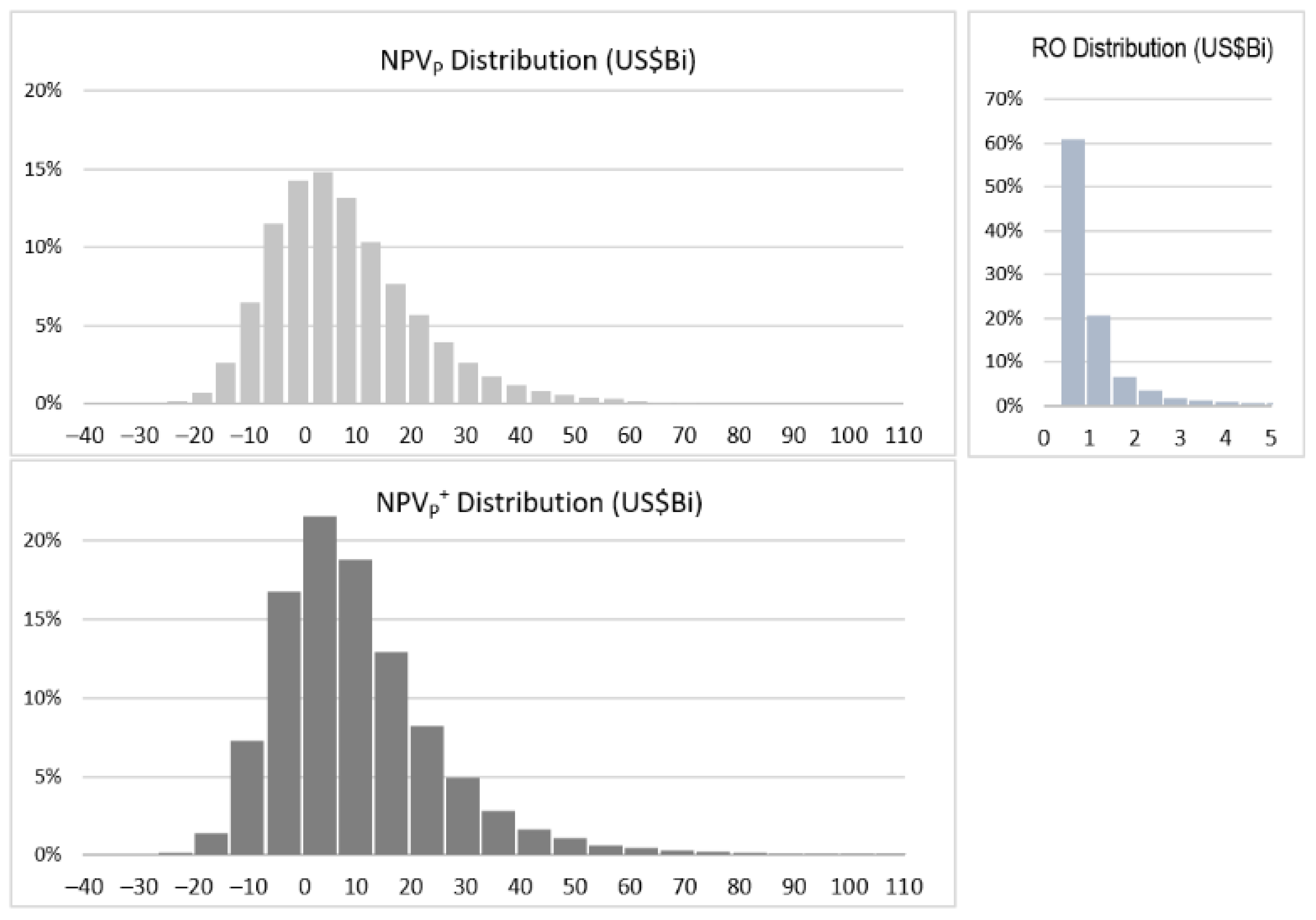
Figure 1 shows the distribution of the NPV of the portfolio without real options (NPV_P), the distribution of real option values (RO), and the distribution of the NPV of the portfolio with real options $NP{V}_P^{+}$.

Note that in Figure 1, the distribution of real options consists exclusively of positive values, highly concentrated in values below US$1000 MM, which, when added to the NPV_P distribution, results in the portfolio distribution with real options, NPV_P⁺, clearly with a higher kurtosis, thus increasing the mean of the portfolio’s NPV distribution from US$5896.36 MM to US$7251.21 MM.

6. Conclusions

The correct analysis of risk, return, and performance of a portfolio of investment projects is of crucial importance in managerial decision-making. The more flexible the valuation techniques and models used, the greater the company’s ability to react to favorable or unfavorable circumstances.

The main objective of this study was to propose a methodology to optimize a portfolio of investment projects using the Omega measure, considering the possibility of including real options in the analysis. Among the main contributions of the proposed methodology are (1) optimization by maximizing the Omega performance measure, which takes into account all moments of the projects’ NPV distribution instead of only the mean and variance, and (2) extension of the Marketed Asset Disclaimer—MAD—assumption (Copeland and Antikarov 2003) from an asset to a set of investment projects taking into account the existing correlations among the input variables that compose the cash flows, and the resulting present values of the projects.

The methodology was illustrated with a numerical application for a company with soybean fields and soybean oil production plants. European, real options were included to increase the value of the projects. The results show that the best ratio of expected gains to expected losses was achieved with the optimization methodology proposed here, being a more realistic approach than simplifying the analysis by mean and variance, as the classic portfolio selection methodology proposes. Other types could also be considered in relation to the exemplified real options, such as sequential options, simultaneous options, and/or temporary interruption of the investment. The real options to be chosen will depend on the particular characteristics of the investment projects that comprise the portfolio, thus making the evaluation of investments closer to reality.

The proposed methodology is flexible, as it allows modeling of the risk variables in different ways. In the present work, we performed the modeling based on stochastic processes, but other types of modeling could be adopted, such as econometric modeling, if this approach better reflects the behavior of the risk variable. It will be up to the analyst to choose the most appropriate way to model a variable.

References

1. Anand, Jaideep, Raffaele Oriani, and Roberto S. Vassolo. 2007. Managing a portfolio of real options. Advances in Strategic Management 24: 275–303. [Google Scholar] [CrossRef]
2. Bernard, Carole, Steven Vanduffel, and Jiang Yeb. 2019. Optimal strategies under Omega ratio. European Journal of Operational Research 275: 755–67. [Google Scholar] [CrossRef]
3. Bhattacharyya, Rupak, Amitava Chatterjee, and Samarjit Kar. 2010. Uncertainty theory based novel multi-objective optimization technique using embedding theorem with application to R&D project portfolio selection. Applied Mathematics 1: 189–99. [Google Scholar] [CrossRef] [Green Version]
4. Brandão, Luiz E., James S. Dyer, and Warren J. Hahn. 2005. Response to Comments on Brandão et al. (2005). Decision Analysis 2: 103–9. [Google Scholar] [CrossRef] [Green Version]
5. Brealey, Richard A., Stewart C. Myers, and Franklin Allen. 2016. Principles of Corporate Finance, 12th ed. New York, NY: McGraw-Hill/Irwin. [Google Scholar]
6. Brosch, Rainer. 2001. Portfolio-aspects in real options management: Working Paper Series: Finance & Accounting, Johann Wolfgang Goethe-Universität Frankfurt am Main. Available online: https://www.econstor.eu/bitstream/10419/76954/1/wp066.pdf (accessed on 15 January 2021).
7. Carazo, Ana F., Trinidad Gómez, Julián Molina, Alfredo G. Hernández-Díaz, Flor M. Guerrero, and Rafael Caballero. 2010. Solving a comprehensive model for multiobjective project portfolio selection. Computers & Operations Research 37: 630–39. [Google Scholar] [CrossRef]
8. Castro, Javier, Edison A. Tito, Luiz E. Brandão, and Leonardo L. Gomes. 2020. Crypto-assets portfolio optimization under the omega measure. Engineering Economist 65: 114–34. [Google Scholar] [CrossRef]
9. Copeland, Tom, and Vladimir Antikarov. 2003. Real Options, Revised Edition: A Practitioner’s Guide. New York: Texere. [Google Scholar]
10. Dixit, Avinash K., and Robert S. Pindyck. 1994. Investment under Uncertainty. Princeton: Princeton University Press. [Google Scholar]
11. Goel, Anubha, and Aparna Mehra. 2021. Robust Omega ratio optimization using regular vines. Optimization Letters 15: 2067–108. [Google Scholar] [CrossRef]
12. Hassanzadeh, Farhad, Hamid Nemati, and Minghe Sun. 2014a. Robust optimization for interactive multi-objective programming with imprecise information applied to R&D project portfolio selection. European Journal of Operational Research 238: 41–53. [Google Scholar] [CrossRef]
13. Hassanzadeh, Farhad, Mohammad Modarres, Hamid R. Nemati, and Kwasi Amoako-Gyampah. 2014b. A robust R&D project portfolio optimization model for pharmaceutical contract research organizations. International Journal of Production Economics 158: 18–27. [Google Scholar] [CrossRef] [Green Version]
14. Heidenberger, Kurt, and Christian Stummer. 1999. Research and development project selection and resource allocation: A review of quantitative modelling approaches. International Journal of Management Reviews 1: 197–224. [Google Scholar] [CrossRef]
15. Jarque, Carlos M., and Anil K. Bera. 1980. Efficient tests for normality, homoscedasticity and serial independence of regression residuals. Economics Letters 6: 255–59. [Google Scholar] [CrossRef]
16. Kane, S. J., M. C. Bartholomew-Biggs, M. Cross, and M. Dewar. 2009. Optimizing Omega. Journal of Global Optimization 45: 153–67. [Google Scholar] [CrossRef] [Green Version]
17. Kapsos, Michalis, Steve Zymler, Nicos Christofides, and Berç Rustem. 2014. Optimizing the Omega ratio using linear programming. The Journal of Computational Finance 17: 49–57. [Google Scholar] [CrossRef] [Green Version]
18. Kazemi, Hossein, Thomas Schneeweis, and Raj Gupta. 2004. Omega as a performance measure. Journal of Performance Measurement 8: 16–25. [Google Scholar]
19. Keating, Con, and William F. Shadwick. 2002. A universal performance measure. Journal of Performance Measurement 6: 59–84. [Google Scholar]
20. Magazzini, Laura, Fabio Pammolli, and Massimo Riccaboni. 2016. Real Options and Incremental Search in Pharmaceutical R&D Project Portfolio Management. Creativity and Innovation Management 25: 292–302. [Google Scholar] [CrossRef]
21. Maier, Sebastian, Georg C. Pflug, and John W. Polak. 2020. Valuing portfolios of interdependent real options under exogenous and endogenous uncertainties. European Journal of Operational Research 285: 133–47. [Google Scholar] [CrossRef]
22. Mansini, Renata, Wlodzimierz Ogryczak, and M. Grazia Speranza. 2014. Twenty years of linear programming based portfolio optimization. European Journal of Operational Research 234: 518–35. [Google Scholar] [CrossRef]
23. Markowitz, Harry. 1952. Portfolio Selection. Journal of Finance 7: 77–91. [Google Scholar] [CrossRef]
24. Mausser, Helmut, David Saunders, and Luis Seco. 2006. Optimizing Omega. Risk 19: 88–92. [Google Scholar]
25. Medaglia, Andrés L., Samuel B. Graves, and Jeffrey L. Ringuest. 2007. A multi-objective evolutionary approach for linearly constrained project selection under uncertainty. European Journal of Operational Research 179: 869–94. [Google Scholar] [CrossRef]
26. Modarres, Mohammad, and Farhad Hassanzadeh. 2009. A Robust Optimization Approach to R&D Project Selection. World Applied Sciences Journal 7: 582–92. [Google Scholar]
27. Mun, Johnathan. 2020. Real Options Analysis, 3rd ed. California: ROV Press. [Google Scholar]
28. PMI. 2017. A Guide to the Project Management Body of Knowledge: PMBOK Guide, 6th ed. Newtown Square, PA: Project Management Institute. [Google Scholar]
29. Samuelson, Paul A. 1965. Proof That Properly Anticipated Prices Fluctuate Randomly. Industrial Management Review 6: 41–49. [Google Scholar]
30. Sefair, Jorge A., and Andrés L. Medaglia. 2005. Towards a model for selection and scheduling of risky projects. Paper presented at 2005 IEEE Design Symposium, Systems and Information Engineering, Charlottesville, VA, USA, April 29; pp. 158–64. [Google Scholar] [CrossRef]
31. Sharpe, William F. 1966. Mutual Fund Performance. The Journal of Business 39: 119–38. [Google Scholar] [CrossRef]
32. Smith, James E. 2005. Alternative Approaches for Solving Real-Options Problems: (Comment on Brandao et al. 2005). Decision Analysis 2: 89–102. [Google Scholar] [CrossRef] [Green Version]
33. Smith, James, and Rex Thompson. 2008. Managing a portfolio of real options: Sequential exploration of dependent prospects. The Energy Journal 29: 43–61. [Google Scholar] [CrossRef] [Green Version]
34. Trigeorgis, Lenos. 1996. Real Options: Managerial Flexibility and Strategy in Resource Allocation. Cambridge, MA: The MIT Press. [Google Scholar]
35. Van Bekkum, Sjoerd, Enrico Pennings, and Han Smit. 2009. A real options perspective on R&D portfolio diversification. Research Policy 38: 1150–58. [Google Scholar] [CrossRef] [Green Version]
36. Vilkancas, Renaldas. 2014. Characteristics of Omega-Optimized Portfolios at Different Levels of Threshold Returns. Business, Management and Education 12: 245–65. [Google Scholar] [CrossRef] [Green Version]
Figure 1. Distribution of NPV of the portfolio with and without real options (US$Bi).
Jrfm 14 00530 g001