An Investigation into the Sources of Depreciations in Mongolian Tugrik Exchange Rate: A Structural VAR Approach

Abstract

This paper empirically investigates the sources of fluctuations in real and nominal Mongolian Tugrik (MNT) exchange rates by estimating the structural vector autoregressive (SVAR) model over the period January 1994–May 2021 and decomposing the exchange rate series into stochastic components induced by real and nominal shocks under the assumption of the long-run neutrality of nominal shocks on the real exchange rate level. The empirical results show that the real MNT exchange rate movements are primarily due to the real shocks, while the nominal shocks have a major role in explaining nominal exchange rate movements in the short and long run. The nominal exchange rate shows a delayed over-shooting occurring between one and three years after a nominal shock hits the economy. The long-run effect of a monthly one standard deviation nominal shock on nominal MNT exchange rate is 2.5%, which results in a permanent divergence between real and nominal MNT exchange rate and causes non-cointegrated relation between real and nominal MNT exchange rates. The historical decomposition of forecast error indicates that the nominal shock plays a significant role in explaining the depreciation in nominal MNT exchange rate over the last three decades. Our recommendation is to stop “cash handling” policy, minimize monetary shock, and coordinate fiscal and monetary policies to avoid large nominal depreciation.

1. Introduction

Exchange rate may be the most discussed topic in international economics. Numerous papers haven been written in this field since the collapse of the Bretton Woods system, and the study dimensions have been expanding rapidly. One dimension we emphasize here is to disentangle nominal and real shocks in the exchange rate series. This paradigm emerged from the methodological (Blanchard and Quah 1989; King et al. 1991) and theoretical (Dornbusch 1976; Stockman 1987, 1988) advancements in times series econometrics and exchange rate theory, respectively. Lastrapes (1992) first studied the exchange rate fluctuations of six advanced economies by decomposing exchange rate series into real and nominal components by identifying real and nominal shocks using a bivariate structural vector autoregressive (SVAR) model under the assumption of long-run neutrality of nominal shocks on the real exchange rate level. Further, this approach was applied for selected advanced economies (Enders and Lee 1997), for selected transition economies (Dibooglu and Kutan 2001), for emerging economies (Chowdhury 2004), for central and east European advanced and transition economies (Morales-Zumaquero 2006), for east Asian economies (Ok et al. 2010), for Saudi Arabia (Aleisa and Dibooĝlu 2002) and for India (Moore and Pentecost 2006) to explain the sources of exchange rate fluctuations in these countries. To the best of our knowledge, this type of study has not yet been conducted for the Mongolian Tugrik (MNT) exchange rate, which has depreciated substantially over the last three decades (Figure 1).

The defining features of the current state of the Mongolian economy are a mining boom and external indebtedness (Ganbayar 2021). Following the recent huge mining developments, the Government of Mongolia (GoM) implemented several “cash handling” policies to distribute mining income to citizens (Dagys et al. 2020; Yeung and Howes 2015). As a result of these cash handling policies, the money supply in Mongolia increased substantially (Figure 2). On the other hand, the skyrocketed external debt (Batsuuri 2015; Ganbayar 2021), which is primarily in US dollars, causes the Bank of Mongolia (BoM) to manage exchange rate depreciation to secure confidence in domestic currency despite its inflation targeting mandate because there might be an epidemic of the “fear of floating” (Calvo and Reinhart 2002; Taguchi and Gunbileg 2020). As a consequence, the de facto exchange rate arrangement of BoM was recently reclassified twice: (1) to crawl-like from floating, effective 18 September 2017, and (2) to other managed from crawl-like, effective 11 April 2018, according to the International Monetary Fund (IMF (2020)). Under this background, the identification of driving sources of MNT exchange rate depreciation is crucial for coordinating fiscal and monetary policy, participating effectively in exchange rate markets and understanding MNT exchange rate fluctuations. Hence, the main purpose of this study is to empirically identify the sources of substantial depreciation in MNT exchange rate over the last three decades by decomposing both real and nominal MNT exchange rate series into nominal and real components using a bivariate SVAR model, as applied in Lastrapes (1992) and Enders and Lee (1997). Our contribution is to enrich the international economic literature with the empirical evidence of the Mongolian economy, which has rarely been mentioned in international economic literature, and to make reasonable recommendations to the country’s exchange rate policy, especially for the coordination between fiscal and monetary policies.

The remainder of the paper is organized as follows. In the next section, we provide background facts related to our context. Section 3 reviews past literature. In Section 4, we present our empirical model and shock identification strategy. Section 5 provides our data and preliminary analysis. In Section 6, we present our estimation results. Section 7 provides robustness analysis for the empirical results in Section 6. In Section 8, we make conclusions and discuss policy implications of empirical findings.

2. Country Background

Since Mongolia transformed the economic system from a centrally planned economy to a market-based economy in the early 1990s, the Bank of Mongolia (BoM) started implementing a flexible exchange rate regime. The BoM had been adopting monetary aggregate targeting with its reserve money being an operational target until 2006. As the linkage between reserve money and inflation became unstable, the BoM introduced an inflation targeting framework in 2007. In this framework, the BoM, like other inflation targeting central banks, equipped the policy mandates of announcing a mid-term targeted inflation rate to the public and of taking every possible measure to maintain the inflation rate within its targeted range (Taguchi and Gunbileg 2020). According to the principle of the “policy trilemma”, an economy has to give up one of three goals: fixed exchange rate, independent monetary policy, and free capital flows (Fleming 1962; Mundell 1963). Thus, given the free capital mobility in Mongolia, the BoM faces a trade-off in their policy targets between exchange-rate stability and price stability.

While the de jure exchange rate arrangement of Mongolia is floating, the de facto exchange rate arrangement was recently reclassified twice: (1) to crawl-like from floating, effective 18 September 2017, and (2) to other managed from crawl-like, effective 11 April 2018, as reported in IMF (2020). Even though the BoM has been conducting inflation-targeting monetary policies since 2007, the significant depreciation in MNT exchange rate (see Figure 1) receives greater attention from Mongolian policy makers because there might be an epidemic case of the “fear of floating” (Calvo and Reinhart 2002) that comes from a lack of confidence in currency value, especially given that their high external debt is primarily denominated in US dollars because of the “original sin” hypothesis (Eichengreen and Hausmann 1999). In fact, the BoM intervenes in foreign exchange markets by organizing auctions between commercial banks every Tuesday and Thursday. However, despite the substantially increased external debt in Mongolia (Batsuuri 2015; Ganbayar 2021), the data show that there is insignificant fear of floating in the monetary policy rule of the BoM (Taguchi and Gunbileg 2020). Since the BoM has started managing MNT rate recently according to the IMF (2020), determining the sources of exchange rate fluctuation is vital to participate in foreign exchange rate market effectively.

Another point we mention here is the recent mining boom in the Mongolian economy. Following the giant mining developments, the Government of Mongolia (GoM) implemented cash handling policies to distribute mining income (tax, royalty, and dividend) across Mongolian citizens (Dagys et al. 2020; Yeung and Howes 2015). The GoM conducted cash handling policies by creating new vehicles. The largest is the “Human Development Fund”, through which every Mongolian citizen received the benefits of 1 million MNT between 2010 and 2012. The most recent indirect cash handling action backed by mining income was the one-time forgiveness of pension-backed debts in January 2020. At the time of loan cancelation, there were 229.4 thousand pensioners who had taken loans worth 763.3 billion MNT (Ganbayar 2021). These direct and indirect cash handling policies implemented by the GoM increase money supply (nominal shock) substantially and may cause large depreciations in nominal MNT exchange rate (see Figure 2). Figure 2 shows the relative money supply of Mongolia compared to that of China, which is the most integrated country with Mongolia in terms of international trade measures. 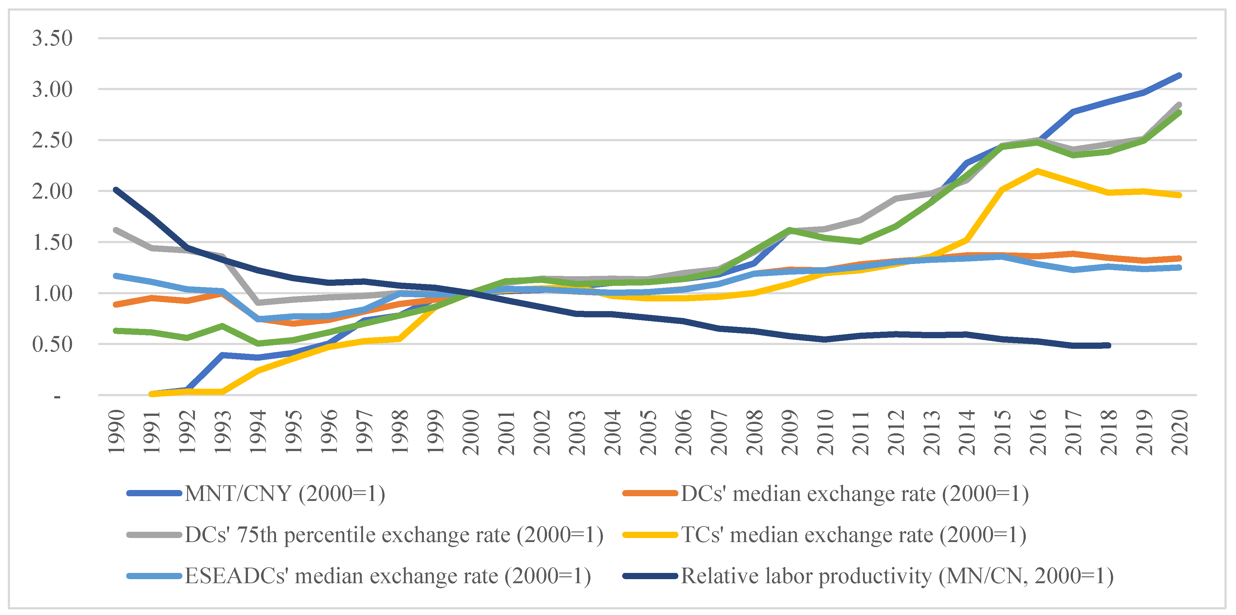In fact, 90% of Mongolia’s total export and 30% of its total import (based on average share over the period 2005–2020, see Supplementary File) belong to China. Both M2 and M1 aggregates indicate that the money supply increased significantly in Mongolia over the last two decades. More specifically, relative M2 and M1 aggregates have increased by 6.8 and 4.2 times since 2000, respectively. These stylized facts imply that the nominal shocks may have a significant effect on the depreciation in nominal MNT exchange rate over the last three decades. The nominal MNT/CNY (per Chinese Yuan in terms of Mongolian Tugrik) exchange rate depreciated by a factor of 3.4 times over the same period (Figure 2). This pattern also works in nominal effective exchange rate (NEER); the NEER is depreciated by 2.45 times. Therefore, it is crucial to determine nominal shocks’ contribution to the evolution of MNT exchange rates.

In addition to nominal factors mentioned above, real factors such as productivity have some role in exchange rate movements (Balassa 1964; Samuelson 1964). Figure 1 shows the relative labor productivity of Mongolia to China. Relative labor productivity of Mongolia decreased by four times over the last three decades. This productivity decline implies that the traded sectors’ competitiveness is deteriorated significantly relative to China, causing real depreciation in MNT exchange rate due to the decrease in non-traded sector’s prices. In contrast, the mining sector’s boom in Mongolia tends to result in real appreciation in MNT exchange rate due to the Dutch disease effect (Corden 1984; Ganbayar 2021). If the productivity effect dominates the Dutch disease effect, Mongolia experiences real depreciation and vice versa, ceteris paribus. Therefore, it is inevitable to determine the net effects of real shocks, including productivity and mining shocks, on the movements of MNT exchange rate.

3. Literature Review

Huizinga (1987) first empirically decomposed the real US dollar (USD) exchange rate series into transitory and permanent components using Beveridge–Nelson decomposition (Beveridge and Nelson 1981). The results showed that the real exchange rate is a mean-reverting unit root process and that most of the variance of changes in real USD exchange rate is attributed to permanent components. Since Huizinga (1987) employs the univariate decomposition method, this approach omits some important information contained in other macroeconomic variables, such as nominal exchange rate.

Blanchard and Quah (1989) developed a new approach to decompose output series into transitory (demand) and permanent (supply) components, assuming long-run neutrality of demand shocks on the output level. Using the Blanchard and Quah (1989) method, Lastrapes (1992) first disentangled real and nominal shocks in the exchange rate series using the bivariate SVAR model under the assumption of the long-run neutrality of nominal shocks on the real exchange rate level. This decomposition approach was developed based upon both the equilibrium (Stockman 1987, 1988) and disequilibrium (Dornbusch 1976) theory of exchange rate. According to the equilibrium theory, the real shocks have a power to explain changes in real and nominal rates in both the short and long run. On the other hand, the disequilibrium theory emphasizes the role of nominal shocks in the evolution of real and nominal rates as the exchange rate market responds to the monetary disturbances promptly due to the price rigidity in goods and service markets. Because of this difference in the adjustment speed of these markets to the monetary disturbances, the nominal exchange rate shows an over-shooting dynamic according to the disequilibrium theory developed by Dornbusch (1976). As reported in Lastrapes (1992), the fluctuations of nominal and real exchange rates in advanced economies between March 1973 and December 1989 are due primarily to real shocks. Clarida and Gali (1994) modified Lastrapes (1992)’s approach by setting triangular long-run restriction on a trivariate SVAR model and decomposed the real exchange rate series into three sources induced by supply, demand, and monetary shocks. The literature related to Clarida and Gali (1994) is primarily focused on the drivers of real exchange rate fluctuations. Therefore, these studies exist in a different vein of literature from the objective of our study because we aim to decompose both real and nominal exchange rates into real and nominal components. Therefore, we concentrate here on the literature applying the same approach as Lastrapes (1992), which are discussed in the following paragraphs.

Enders and Lee (1997) decomposed US dollar real and nominal exchange rate movements into the components induced by real and nominal shocks. They found that the real shocks explain a majority of real and nominal exchange rate fluctuations and that there is little evidence of exchange rate over-shooting in bilateral exchange rates between the US and Canada, Japan, and Germany over the period January 1973–April 1992. Dibooglu and Kutan (2001) conducted a similar study for two transition economies, Poland and Hungary. Using monthly real exchange rate and inflation series between January 1990 and March 1999, they found that nominal shocks had a larger influence in explaining real exchange rate movements in Poland, while real shocks had more influence on real exchange rate movements in Hungary. The empirical results imply that sticky-price disequilibrium models explain the behavior of the real exchange rate of Poland, while equilibrium exchange rate models are more suitable for Hungary.

Aleisa and Dibooĝlu (2002) estimated a bivariate SVAR model using monthly data from January 1980 to February 2000 to investigate the sources of real exchange rate movements in Saudi Arabia. Their results suggest that real shocks play a significant role in explaining real exchange rate movements, while nominal shocks play a significant role in explaining price level movements in Saudi Arabia. Moore and Pentecost (2006) conducted the same study on the Indian Rupee against the US dollar over the period from March 1993 through January 2004. The authors found that real and nominal Rupee exchange rates are driven mostly by real shocks and suggested that Indian policy makers need to focus on the real side of the economy in order to stabilize the foreign exchange market.

Chowdhury (2004) studied the sources of real and nominal exchange rate fluctuations in six emerging market countries: Chile, Columbia, Malaysia, Singapore, South Korea, and Uruguay. The author employed exactly the same SVAR model applied in Lastrapes (1992) using monthly observations from January 1980 to December 1996. The empirical results showed that real shocks result in long-run real and nominal appreciation, while nominal shocks generally cause a nominal depreciation. Latin American exchange rates appear to be more sensitive to real and nominal shocks than East Asian exchange rates, according to Chowdhury (2004), because real and nominal shocks have stronger influences on the exchange rates of Latin American countries. Morales-Zumaquero (2006) investigated sources of real exchange rate fluctuations for selected advanced economies—Canada, Japan, US, UK, France, Italy, and Germany—and Central and Eastern European transition economies—Czech Republic, Hungary, Poland, Romania, and Slovenia. Based on the findings of this study, for advanced economies, real shocks account for the majority of exchange rate fluctuations over the period from January 1973 to December 1990, while nominal shocks play a central role in explaining exchange rate movements over the period from January 1991 to January 2000. The author further stated that nominal shocks have a major role in explaining real exchange rate fluctuations for Euro Zone countries over the subperiod January 1991—January 2000 due to the “single monetary policy” of these countries. As the transition economies have different initial conditions and economic policies, the real exchange rate movements in some transition economies (Czech Republic, Hungary, and Slovenia) are explained mostly by real shocks, while in others (Poland and Romania), nominal shocks play a larger role in explaining real exchange rate movements. Ok et al. (2010) investigated the sources of fluctuations in real and nominal US dollar exchange rates in Cambodia and Laos. Their findings were that real shocks have a significant impact on real and the nominal exchange rates, while nominal shocks induce long-run nominal changes and short-run real changes. Laos experiences relatively larger responses to the nominal shock than Cambodia because the exchange rates in an economy with higher inflation respond to the nominal shock more extremely, according to Ok et al. (2010).

4. The Empirical Model

The empirical model identifying real and nominal shocks from the observed real and nominal exchange rate data is given as a bivariate SVAR model in Equation (1) if log of real ($y_t^1$) and log of nominal ($y_t^2$) exchange rates are not cointegrated.

$$\mathsf{\Delta }{y}_t=B_0\mathsf{\Delta }{y}_t+B_1\mathsf{\Delta }{y}_{t-1}+\cdots +B_k{y}_{t-k}+{\epsilon }_t$$

(1)

where $\mathsf{\Delta }{y}_t={\left[\mathsf{\Delta }{y}_t^1\mathsf{\Delta }{y}_t^2\right]}^{\prime }$ is $2\times 1$ column vector, ($\mathsf{\Delta }{y}_t^1$) and ($\mathsf{\Delta }{y}_t^2$) are the first differences of log of real and nominal exchange rates, respectively, $B_0=\left[\begin{array}{cc}0& b_{12}\\ b_{21}& 0\end{array}\right]$ is 2 × 2 square matrix modeling the contemporaneous relation between $\mathsf{\Delta }{y}_t^1$ and $\mathsf{\Delta }{y}_t^2$, $B_1,B_2,\dots ,B_k$ are unrestricted parameter matrix, and $k$ is the sufficient lag length ensuring that structural shocks ${\epsilon }_t={\left[{\epsilon }_t^1{\epsilon }_t^2\right]}^{\prime }$ are serially uncorrelated processes with diagonal variance–covariance matrix: $E{\epsilon }_t^1{{\epsilon }_t^2}^{\prime }=H=\left[\begin{array}{cc}{h}_{11}& 0\\ 0& h_{22}\end{array}\right]$. If we find all coefficient matrixes, $B_0,B_1,\dots B_k$, the real (${\epsilon }_t^1$) and nominal (${\epsilon }_t^2$) shocks will be identified. However, we are not able to recover parameters from observed data using (1) due to the simultaneous equation bias. Hence, we transform (1) to the reduced form (2) by multiplying both sides of (1) with ${\left(I-B_0\right)}^{-1}$, where $I$ is an identity matrix.

$$\mathsf{\Delta }{y}_t=A_1\mathsf{\Delta }{y}_{t-1}+A_2\mathsf{\Delta }{y}_{t-2}+\cdots +A_k{y}_{t-k}+u_t$$

(2)

where $A_i={\left(I-B_0\right)}^{-1}{B}_i$ and $u_t={\left(I-B_0\right)}^{-1}{\epsilon }_t$. We can apply ordinary least square (OLS) estimator on Equation (2) and estimate reduced form parameters, $A_1,A_2,\dots ,A_k$, and variance–covariance matrix $\mathsf{\Sigma }=E{u}_t{u}_t^{\prime }=\left[\begin{array}{cc}{\sigma }_{11}& {\sigma }_{12}\\ {\sigma }_{21}& {\sigma }_{22}\end{array}\right]$. Without one more restriction on the structural model (1), we are not able to recover four structural parameters ($b_{12},b_{12},h_{11}$ and $h_{22}$) from the estimated three reduced form parameters (${\sigma }_{11},{\sigma }_{12}={\sigma }_{21},{\sigma }_{22})$. A simple choice for that restriction is to set $b_{12}$ or $b_{21}$ equal to zero. This is called short-run restriction in time series literature in Sims (1980). As Sims (1980) identification is not theoretically rational for our context, we apply long-run restriction established in Blanchard and Quah (1989).

To set long-run restriction on SVAR model (1), the reduced form model (2) needs to be written in moving average (MA) form by inverting the reduced form model (1) as (3).

$$\mathsf{\Delta }{y}_t={\left(I-A_{1}L-A_2{L}^2\dots -A_k{L}^k\right)}^{-1}{u}_t$$

(3)

where $I$ is a $2\times 2$ identity matrix and $L$ is lag operator. It is worth noting that the reduced form model (2) could be written in MA form (3) given only that $\mathsf{\Delta }{y}_t^1$ and $\mathsf{\Delta }{y}_t^2$ are stationary. Further, we can define ${\left(I-A_{1}L-A_2{L}^2\dots -A_k{L}^k\right)}^{-1}=C\left(L\right)$, which is a matrix of infinite order lag polynomials, as (4).

$$\mathsf{\Delta }{y}_t=C\left(L\right)u_t=\left[\begin{array}{cc}{C}_{11}\left(L\right)& C_{12}\left(L\right)\\ C_{21}\left(L\right)& C_{22}\left(L\right)\end{array}\right]\left[\begin{array}{c}{u}_t^1\\ u_t^2\end{array}\right]$$

(4)

where $u_t^1$ and $u_t^2$ are reduced form residuals. Equation (4) is the MA representation of reduced form (2). We can transform first difference form (4) to level form (5) by multiplying both sides of (4) with ${\left(1-L\right)}^{-1}$ as follows:

$$y_t={\left(1-L\right)}^{-1}C\left(L\right)u_t={\left(1-L\right)}^{-1}C\left(L\right){\left(I-B_0\right)}^{-1}{\epsilon }_t.$$

(5)

From the level form (5), the long-run effect of structural shocks on $y_t$ is

$$\underset{s\to \infty }{\lim }\frac{\partial y_t}{\partial {\epsilon }_{t-s}}=C\left(1\right){\left(I-B_0\right)}^{-1}{\epsilon }_t.$$

(6)

The neutrality assumption of nominal shocks on the long-run value (level) of real exchange rates requires that the matrix $C\left(1\right){\left(I-B_0\right)}^{-1}$ be lower triangular. As a result of this triangular restriction, we have

$$b_{12}=-\left[C_{12}\left(1\right)/C_{11}\left(1\right)\right].$$

(7)

Since we identify $b_{12}$ from long-run restriction, the remaining three structural parameters are just identified from the following system of three equations by substituting the value of $b_{12}$ into the system (8a)–(8c).

$${\sigma }_{11}-2b_{12}{\sigma }_{12}+b_{12}^2{\sigma }_{22}-h_{11}=0$$

(8a)

$$-b_{21}{\sigma }_{11}+\left(1+b_{12}{b}_{21}\right){\sigma }_{12}-b_{12}{\sigma }_{22}=0$$

(8b)

$$b_{21}^2{\sigma }_{11}-2b_{21}{\sigma }_{12}+{\sigma }_{22}-h_{22}=0$$

(8c)

5. The Data

During the early years of transition from centrally planned economy to market-based economy, MNT nominal exchange rate depreciated substantially (Figure 2) and consumer price index (CPI) skyrocketed due to the government abandoning control of price and exchange rate. Therefore, we exclude data before January 1994, because the exchange rate movements during that period were mostly driven by transition effects.

The data used in our study are from the International Financial Statistics (IFS), IMF. We collected seasonally unadjusted monthly nominal exchange rates and seasonally unadjusted monthly consumer price indexes of Mongolia (MN) and China (CN) from January 1994 to May 2021. The nominal exchange rate is the monthly average of MNT per unit of CNY. The real exchange rate is the nominal exchange rate times the ratio of CPI of CN to CPI of MN. In other words, the real exchange rate is the per consumption basket of CN in terms of the consumption basket of MN. Our measure of real exchange rate closely mimics the REER estimated by the BoM between January 2000 and May 2021 (Figure 2), because China weighs heavily in the REER calculation. We take the logarithm of these two variables before making preliminary analysis and estimating SVAR model.

First of all, we perform unit root and cointegration tests in order to ensure that the SVAR is the proper model in our context.

Table 1. Unit root and cointegration test.

Unit Root Test
Test Type	Specification	Level		First Difference
		L. of R. Rate	L. of N. Rate	L. of R. Rate	L. of N. Rate
ADF	None	0.775	4.109	−9.383 ***	−4.254 ***
	Constant	−2.371	−1.881	−9.381 ***	−5.422 ***
	C. and T.	−2.409	−2.582	−9.441 ***	−5.529 ***
PP	None	0.850	4.338	−15.954 ***	−15.228 ***
	Constant	−2.008	−1.765	−123.990 ***	−23.148 ***
	C. and T.	−2.002	−2.559	−181.241 ***	−18.223 ***
Cointegration test
EG	Dependent var.	tau-statistic	Probability	z-statistic	Probability
	L. of N. rate	−0.745	0.939	−1.696	0.944
	L. of R. rate	−1.095	0.883	−4.113	0.800
JC	Unrestricted cointegration rank test based on trace statistic
	# of CE(s)	Eigenvalue	Trace statistic	0.05 C.V.	Probability
	None	0.029	10.156	15.495	0.269
	At most 1	0.004	1.204	3.841	0.273
	Unrestricted cointegration rank test based on maximum eigenvalue
	# of CE(s)	Eigenvalue	M.E. Statistic	0.05 C.V.	Probability
	None	0.029	8.952	14.265	0.290
	At most 1	0.004	1.204	3.841	0.273

Source: Authors’ estimation. Note: L.—logarithm, R.—real, N.—nominal, ADF—augmented Dickey–Fuller test (Dickey and Fuller 1979), PP—Philips–Perron test (Phillips and Perron 1988), EG—Engle–Granger single equation test (Engle and Granger 1987), JC—Johansen cointegration test (Johansen 1991), var.—variable, #—number, CE(s)—cointegration equation(s), C.V.—critical value and M.E.—maximum eigenvalue. *** indicates 1% significance level.

presents the results of unit root tests. Lag lengths of unit root tests are based on Akaike information criteria (AIC). The test statistics of the augmented Dickey–Fuller (ADF) and the Philips–Perron (PP) tests indicate that all of the variables have a unit root in level, as the null hypotheses of unit root are not rejected at the conventional significance level. However, both ADF and PP test statistics reject the presence of unit roots in all variables in the first differences at the 1% significance level. Since the real and nominal exchange rates are I(1) processes, we further need to test cointegrated or long-run relations between these two variables. The Engle–Granger (EG) and Johansen cointegration (JC) test statistics are shown in Table 1. Both EG and JC test statistics indicate that the null hypotheses of no cointegration are not rejected at a conventional significance level. We will discuss why these two series are not cointegrated in the following section. Therefore, we can apply the SVAR model, which is preferred to the structural vector error correction (SVEC) model, in our case.

6. Estimation Result

The reduced form bivariate VAR model (2) is estimated for log difference of real and nominal exchange rate series over the period January 1994–May 2021. Starting with a maximum lag of 24, the optimal lag length (k) is 24 according to three criteria: likelihood ratio test statistic at the 5% significance level, final prediction error, and AIC (see Supplementary File). We test serial correlations in the reduced form residuals using Ljung–Box Q statistics, which affirms that there are no significant serial correlations in reduced form residuals (see Supplementary File). However, the residuals of the reduced form VAR model are correlated with each other such that the contemporaneous pairwise correlation between $u_t^1$ and $u_t^2$ is 0.81 and the corresponding t-statistic is 23.86 (see Supplementary File). This result indicates that there is a reasonable structural relationship between these two series and the SVAR model is appropriate for our context rather than the VAR model. Using (7), (8a)–(8c), we recover parameters of structural model (1) from the estimated reduced form model (2) and calculate structural impulse response functions in Figure 3.

Figure 3a shows that the real exchange rate immediately responds to a real shock such that one standard deviation real shock increases real exchange rate by 3% in two months. The effect of real shock on the real exchange rate decreases gradually and reaches the long-run value of 1.5%, which is obtained at a horizon of about 41 months. The 95% confidence interval from bootstrap simulation with 500 replications for reduced form residuals indicates that the response of real exchange rate to real shocks are statistically significant, implying that the real shocks are the main sources of real exchange rate movements. It is worth noting that the normality assumption does not hold for our structural residuals (see Supplementary File). With non-normal residuals, we could not precisely estimate the confidence interval using analytic formulas. Therefore, we estimated the confidence interval employing the bootstrap simulation method in this study.

Figure 3b shows that the nominal exchange rate also immediately responds to real shocks such that one standard deviation real shock increases nominal exchange rate by 2.2% in one month. The effect of real shocks on nominal exchange rate decreases gradually and reaches the long-run value at a horizon of about 2 years. However, the 95% confidence interval indicates that the response of nominal exchange rate to a real shock becomes statistically insignificant one year after the real shock hits the economy. This pattern could be explained by price adjustment processes in the Mongolian economy. Once a real shock occurs in the economy, the prices of goods and services gradually, though not immediately, adjust due to the price stickiness, while the nominal exchange rate immediately responds to a real shock. When the prices are adjusted significantly, the effect of the real shock on nominal exchange rate becomes insignificant.

The response of the real exchange rate to a nominal shock is insignificant in both short and long horizons as shown in Figure 3c. This result clearly reflects our identification restriction, which is the long-run neutral effect of nominal shocks on the real exchange rate level. In addition, the real MNT exchange rate is unresponsive to a nominal shock in the short run.

Finally, Figure 3d shows the dynamic response of nominal exchange rate to a nominal shock. This indicates that there is a delayed over-shooting behavior in nominal MNT exchange rate. The over-shooting peaks at a horizon of 20 months at close to 3% and gradually declines to the long-run value of 2.4% after about three and half years. In other words, one standard deviation nominal (monetary) shock immediately increases the nominal exchange rate by 1%, 3% after 20 months, and 2.4% in the long run. The reason for the delayed over-shooting could be explained by the intervention of the BoM in foreign exchange rate markets. Once the BoM increases the money supply substantially, the BoM can predict the outcomes in the exchange rate market and try to dilute the short-run influence of the money supply shock on the nominal MNT exchange rate by intervening in foreign exchange markets. As a result of this intervention, the over-shooting time is delayed but the long-run effect of nominal shock becomes larger compared to other previously studied countries. Hence, there could be a trade-off between short-run stabilization and long-run depreciation in MNT exchange rate.

In the previous section, we found that the nominal and real exchange rates are not cointegrated. This finding is consistent with the empirical result in Figure 3 because the nominal shock can lead to a permanent divergence between nominal and real rates. This result is due to the nominal exchange rate’s absorption of nominal shock in both the short and long run, while the real exchange rate is unresponsive to the nominal shock in the long run as well as in the short run.

Overall, the real exchange rate is primarily driven by real shocks, while the nominal exchange rate is mainly driven by nominal shocks. The effect of a real shock on nominal exchange rate is significant in the short run but not in the long run. Therefore, the recent depreciation in nominal MNT exchange rate was mainly caused by nominal shocks, in particular the large money supply induced by the government policies, such as the cash handling policy mentioned earlier. The BoM may sterilize the effect of nominal shock on nominal exchange rate by intervening in this market, because the BoM can predict the outcome of a significantly enlarged money supply. As a result of this sterilization, the nominal MNT exchange rate shows delayed over-shooting, while the nominal MNT exchange rate immediately responds to a real shock, because the BoM cannot predict the real shock as well. Hence, the BoM usually ignores the effects of a real shock on nominal MNT exchange rate.

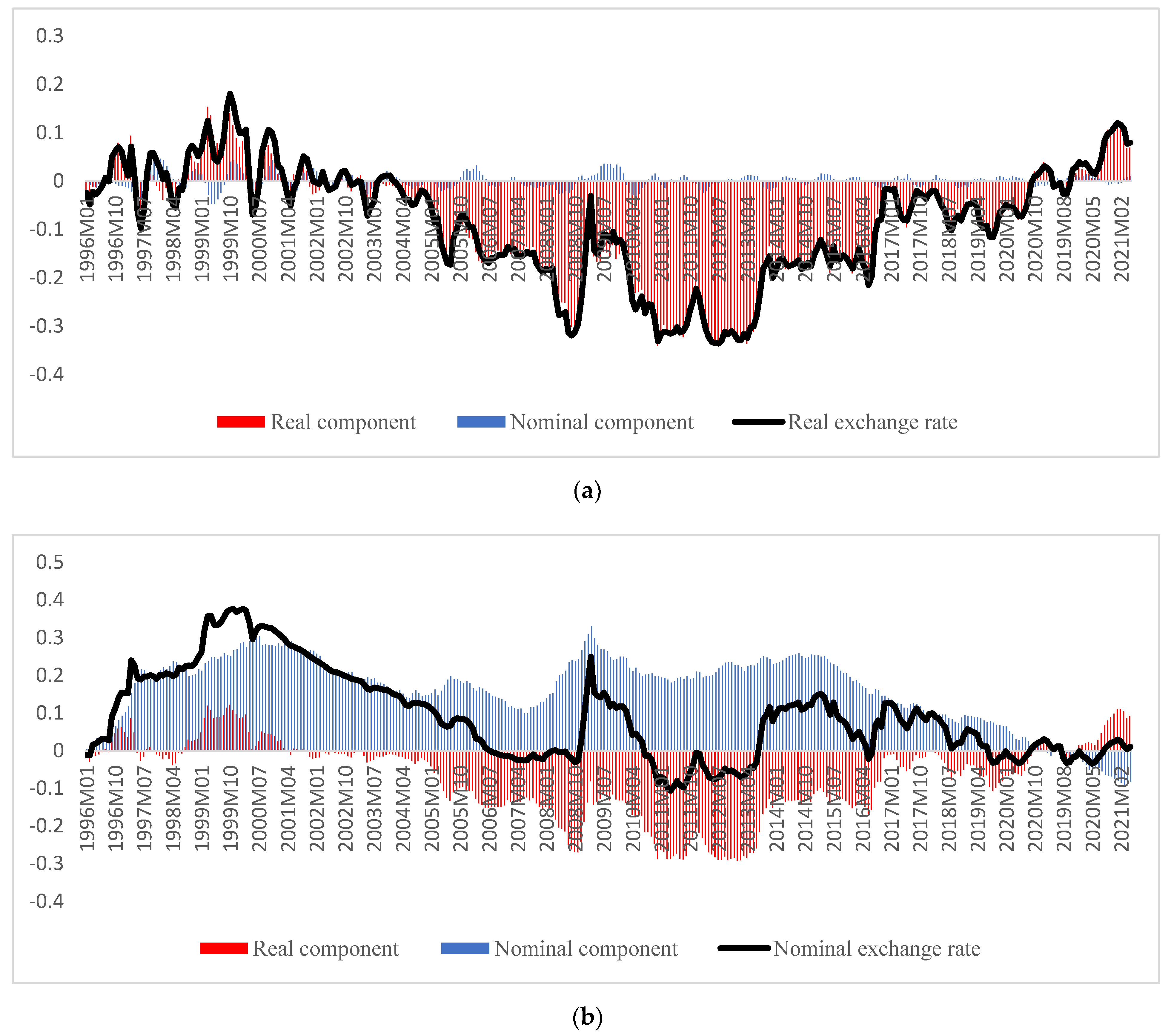
The dynamic responses are consistent with the historical decompositions of forecast errors in Figure 4. Figure 4 decomposes the accumulated 24-month exchange rate forecast error into real and nominal components. The real (nominal) component is obtained by setting all realizations of nominal (real) shocks to zero in Equation (5). Figure 4a shows that the forecast errors in real exchange rate movements are primarily driven by the real components. The Mongolian economy experienced major real appreciations between 2005 and 2017 because the first mining boom started around 2005 and the second began around 2010. Figure 1 shows that the productivity factor causes real depreciation, but the country experienced real appreciation despite the decreasing productivity. This is because the Dutch disease effect caused by the mining boom may dominate the productivity effect if we assume that other factors are relatively small. However, the real appreciation has been placated recently due to the decay of the mining boom and the monotonic fall in relative labor productivity as mentioned earlier.

On the other hand, the nominal component has a major contribution to the forecast error of nominal exchange rate as shown in Figure 4b. We can infer that the substantial depreciations in nominal MNT exchange rate between 1996 and 2020 are mostly driven by nominal shocks. The nominal component would have caused nominal MNT exchange rate to depreciate by at least 10% from its forecasted rate over the period 1996–2017 if there were not an off-setting effect from the real components. In contrast, the real component had an appreciating effect on the nominal MNT exchange rate between 2005 and 2017. The net effect results in nominal depreciation in MNT exchange rate for almost all of the period because the nominal components dominated the real components.

7. Robustness Analysis

The SVAR model can be sensitive to data frequency and sample period (Stock and Watson (2001)). Therefore, we first conducted robustness analysis on the SVAR model estimated in the previous section by changing the frequency of our data from month to quarter. We re-estimated the SVAR model (1) on the quarterly data over the period 1994Q1–2021Q1 by setting the lag to 8 quarters, which is equal to 24 months. The impulse response result is depicted in Figure 5. The patterns of quarterly impulse response closely mimic the monthly patterns.

Further, we re-estimated the SVAR model for the post-inflation targeting period by changing the sample ranges, January 2007–May 2021 and 2007Q1–2021Q1, for monthly and quarterly data, respectively. The impulse responses for the post-inflation sample closely mimic our main result as well (see Supplementary File). Hence, our estimation is robust over the frequency of data and stable over time. We conducted standard structural break tests to justify our robustness analysis in the following paragraph.

To be more formal, we ran standard multivariate structural change tests as developed in Lütkepohl and Krätzig (2004). The structural change test results are reported in

Table 2. Standard structural change test result.

Type of Tests	Test Statistic	95% Critical Value	p-Value
Break-point test	642.8	680.4	0.268
Sample-split test	204.2	264.8	0.758

Source: Authors’ estimation. Note: 95% critical value and p-value are from bootstrap simulation with 1000 replications. Break point date is January 2007, inflation targeting date.

. We selected the inflation targeting date, January 2007, as our suspected structural change date.

Both the break-point test and sample-split test do not reject the null hypothesis of parameter constancy as the corresponding test statistics are less than the 95% critical values and the p-values are greater than 10%. Therefore, our empirical result is stable over time.

8. Conclusions and Discussion

In this study, we decomposed MNT exchange rate series into real and nominal components by identifying real and nominal shocks using a bivariate SVAR model under the assumption of the long-run neutrality of nominal shocks on the real exchange rate level. The IRF result shows that the real exchange rate immediately responds to real shocks, such that one standard deviation real shock increases the real exchange rate by 3% in two months and by about 1.5% in the long run. Therefore, the real shocks have a significant influence on real exchange rate in both the short and long run. The pattern of response of the real exchange rate to the real shock is consistent with other studies, such as Lastrapes (1992), Enders and Lee (1997), and Chowdhury (2004), among others.

Nominal exchange rate also immediately responds to real shocks, but the response gradually decreases and becomes insignificant after 12 months. This is because the prices of goods and services gradually adjust to the real shock due to price stickiness, while the nominal exchange rate immediately responds to the real shock. When the prices are adjusted substantially, the effect of real shocks on nominal exchange rate become insignificant after one year. Hence, we infer that the real shocks have only short-run influence on nominal exchange rate. This result is similar to the impulse response result of Cambodian Riel as estimated in Ok et al. (2010): the Cambodian Riel immediately responds to real shocks.

The response of the real exchange rate to nominal shock is insignificant in both the short and long term. This is consistent with our assumption of the long-run neutrality of nominal shock on the real exchange rate level. Moreover, the nominal shocks have no effect on real exchange rate, even in short run. The insignificant effects of nominal shock on the real exchange rate have been reported in past studies, including Lastrapes (1992), Enders and Lee (1997), Dibooglu and Kutan (2001), Aleisa and Dibooĝlu (2002), Chowdhury (2004), Morales-Zumaquero (2006), and Ok et al. (2010), among others.

The dynamic response of the nominal exchange rate to nominal shock indicates that there is a delayed over-shooting behavior in nominal MNT exchange rate. The over-shooting peaks after about 20 months at close to 3% and reaches a long-run value of 2.4% after about 14 quarters. The absolute value of the over-shooting peak is close to the results of Lastrapes (1992), but the long-run value is greater the those of Lastrapes (1992). This discrepancy between MNT exchange rate and developed countries’ exchange rates could be explained by the intervention of the BoM. The BoM intervenes in the exchange rate market to reduce short-run effects of the nominal shocks on MNT exchange rate. However, this intervention results in a trade-off between short and long run deprecation in MNT exchange rate.

The delayed over-shooting results are reported in Ok et al. (2010) for Cambodian Riel and Laotian Kip. However, the authors did not give reasonable theoretical explanation for this delayed over-shooting patterns. In the case of the Mongolian Tugrik, the reason for the delayed over-shooting could be explained by the intervention of the BoM in foreign exchange rate markets. The cost of the intervention might be the long-run change in nominal MNT rate. Nominal shocks have a significant influence on the nominal exchange rate in the short and long run. This finding explains why nominal and real exchange rates are not cointegrated. In other words, nominal shock leads to a permanent divergent between the nominal and real exchange rates. This result is consistent with the findings of Lastrapes (1992).

These dynamic responses are supported by the historical decompositions of forecast errors. The Mongolian economy experienced major real appreciations, mostly driven by real sources, between 2005 and 2017, because the Dutch disease effect dominates productivity effects. The real exchange rate of MNT has currently depreciated by 8% from the forecasted rate since the country’s productivity did not improve and the second mining boom declined. On the other hand, the nominal component has made a major contribution to the forecast error of nominal exchange rate. We can infer that the substantial depreciations in nominal MNT exchange rate between 1996 and 2020 are mostly due to nominal factors such as money supply.

All in all, the real exchange rate is driven by real shocks, while the nominal exchange rate is driven by nominal shocks in the long run. The depreciation in nominal MNT exchange rate might be caused by nominal shocks, such as the large money supply due to the cash handling policy implemented by GoM. Thus, our first recommendation is to stop cash handling policy, which depreciates MNT exchange rates significantly as a function of the nominal shock. Our second recommendation is to minimize nominal shocks induced by the BoM to manage fluctuations in nominal MNT exchange rate. Finally, the BoM and the GoM should coordinate their policies; the cash handling policy by the GoM and the stable nominal exchange rate policy by the BoM are impossible to achieve at the same time, according to our empirical results.

Several extensions of our empirical findings would be desirable, including constructing small open economy’s New Keynesian dynamic stochastic general equilibrium model for the Mongolian economy to identify real and nominal shocks in detail and using Clarida and Gali’s (1994) approach to decompose real MNT exchange rate into components induced by supply, demand, and monetary shocks. These would be useful topics for future research.