

Revealing the History and Mystery of RNA-Seq
Abstract
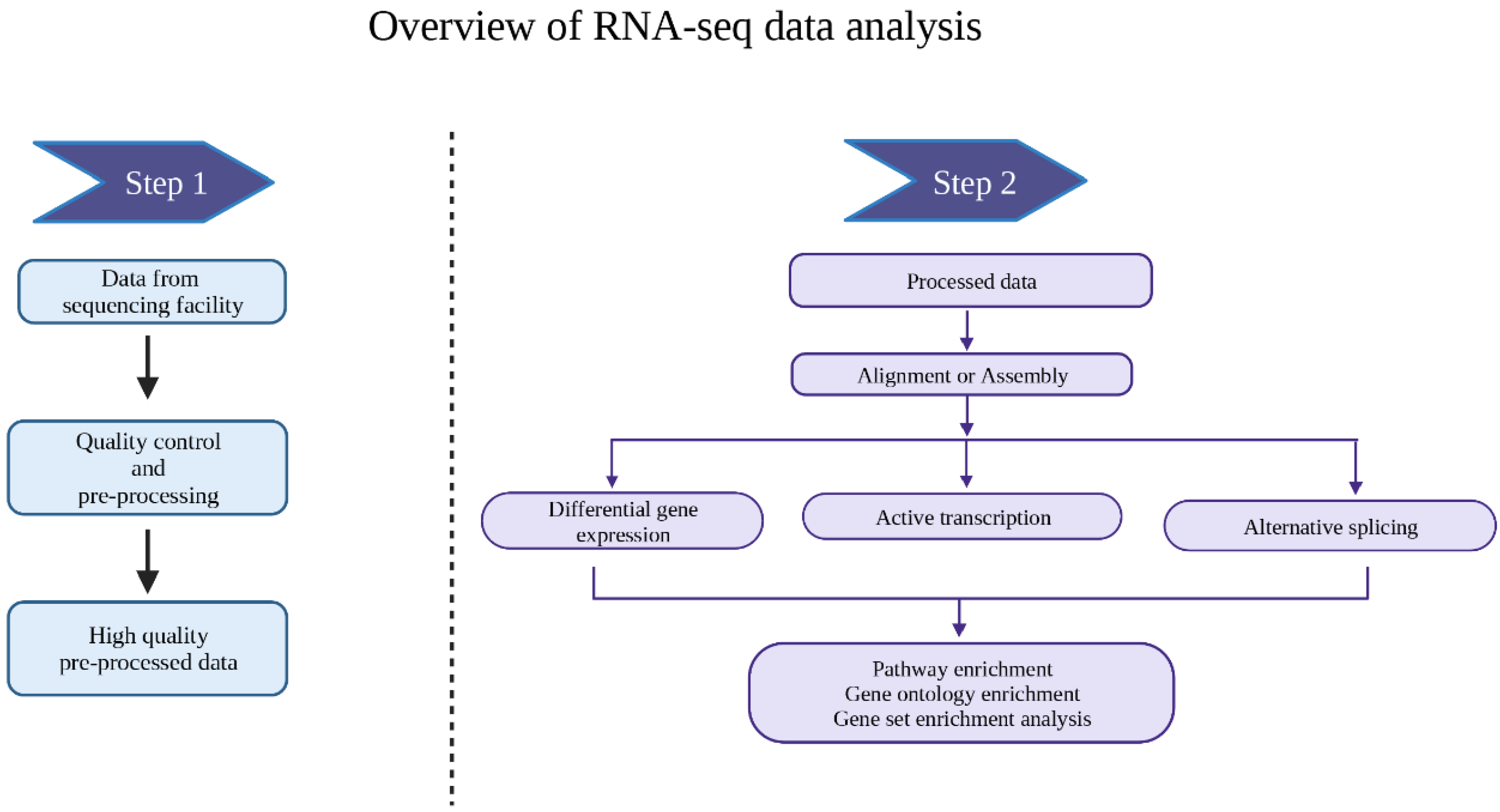
:1. Introduction: Evolution of Sequencing Technologies
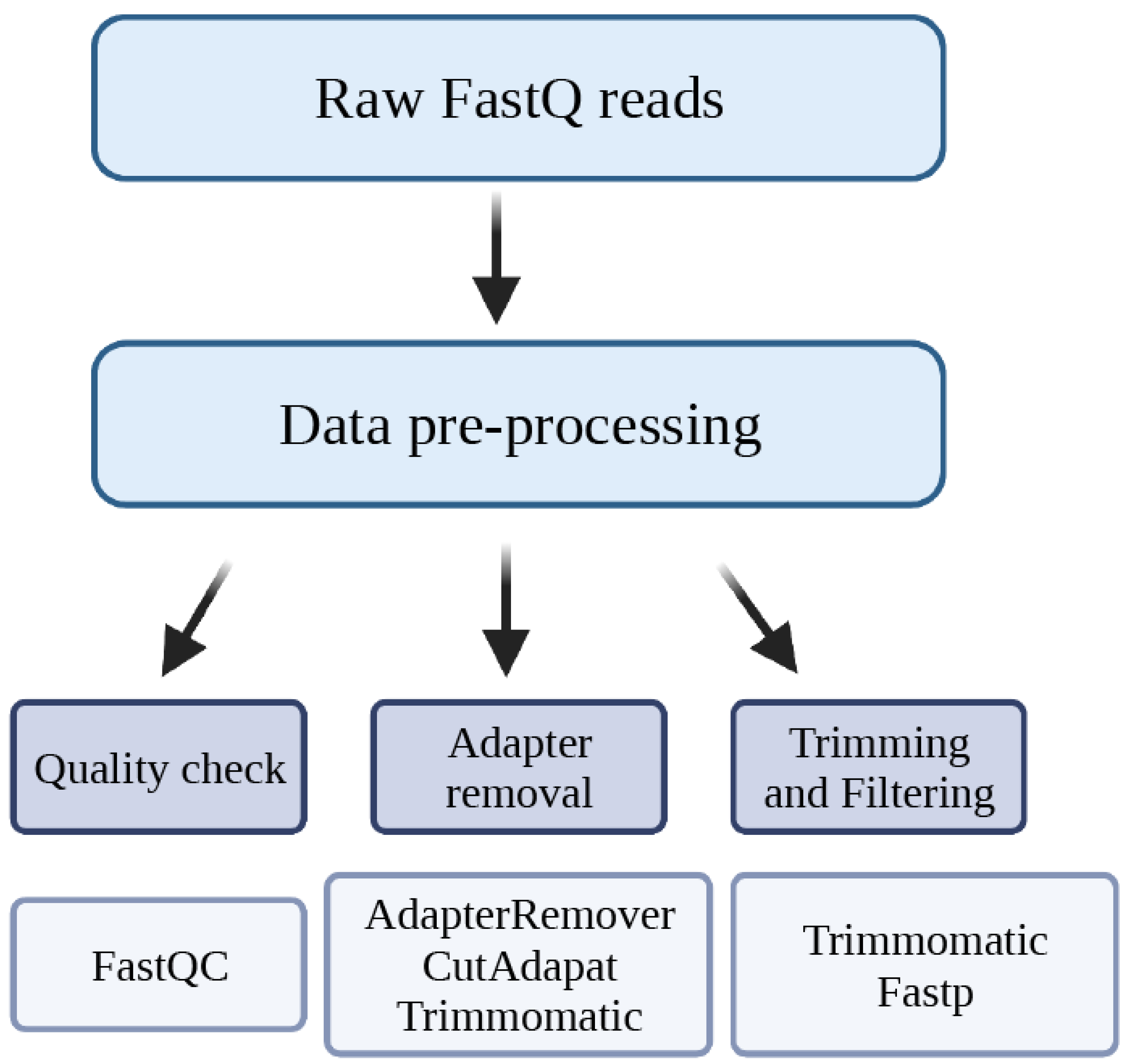
2. Data Pre-Processing
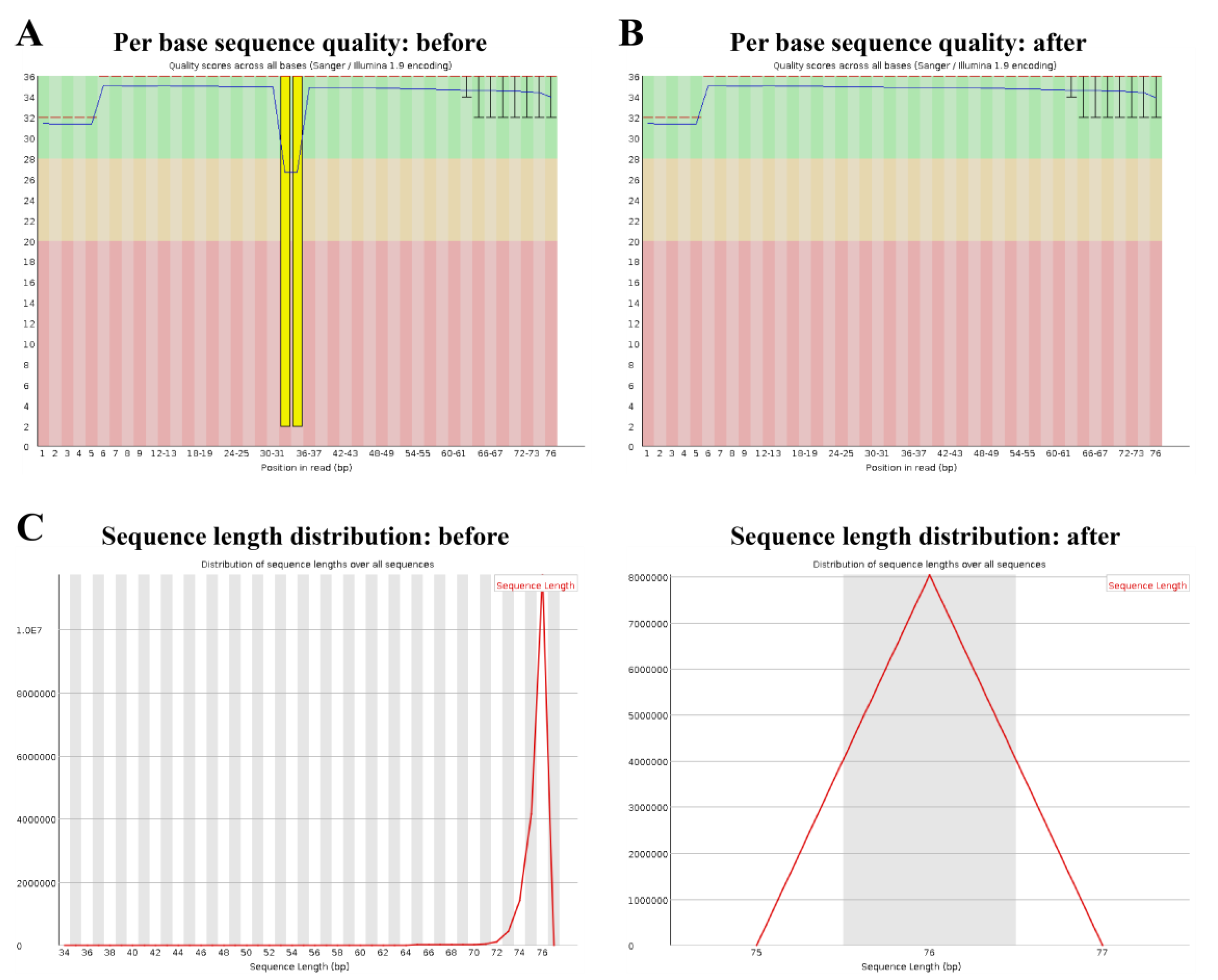
2.1. Quality Check
2.2. Adapter Removal
2.3. Trimming and Filtering
3. Data Analysis
3.1. Alignment
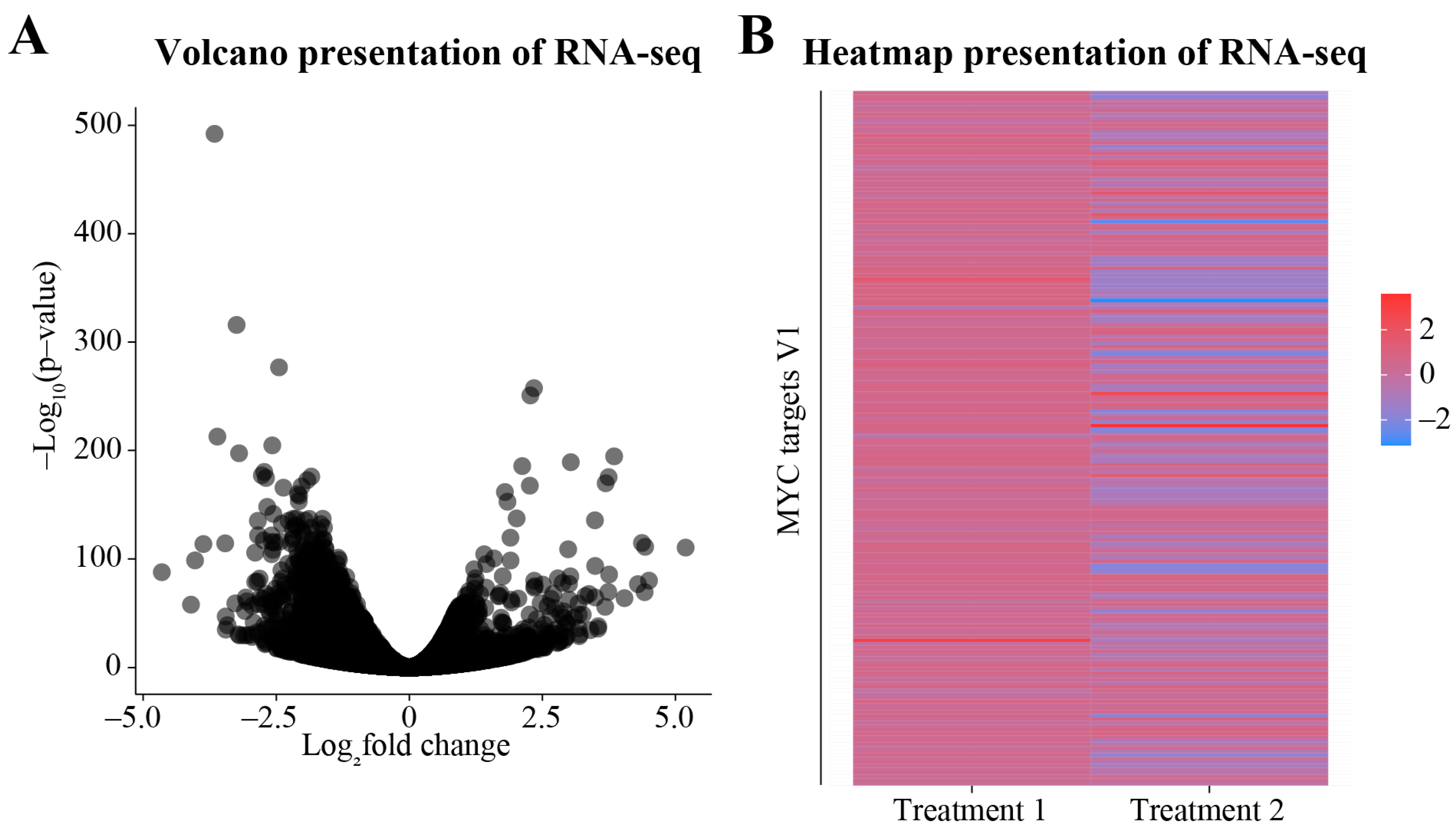
3.2. Differential Gene Expression Analysis
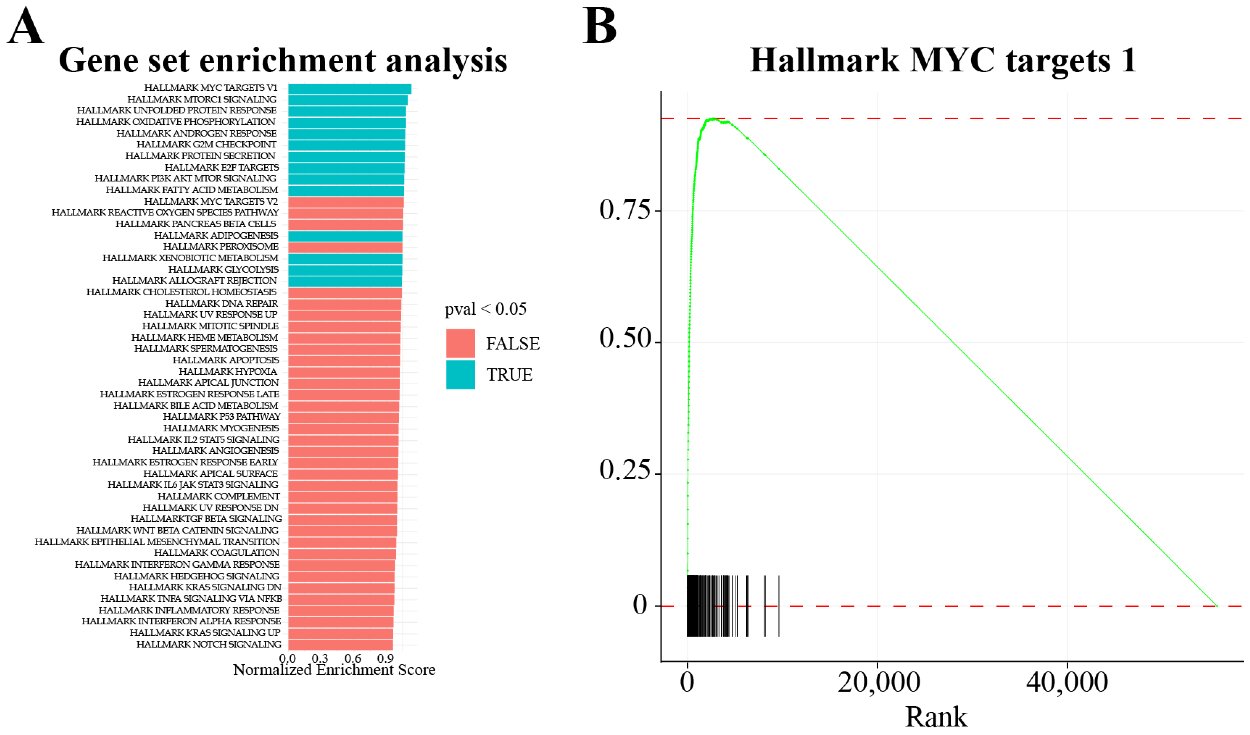
3.3. Downstream Analysis of the DEGs

3.4. Nascent RNA Sequencing Technologies
3.5. Downstream Analysis of the Metabolically Labeled RNA
3.6. Analysis of Alternative Splicing
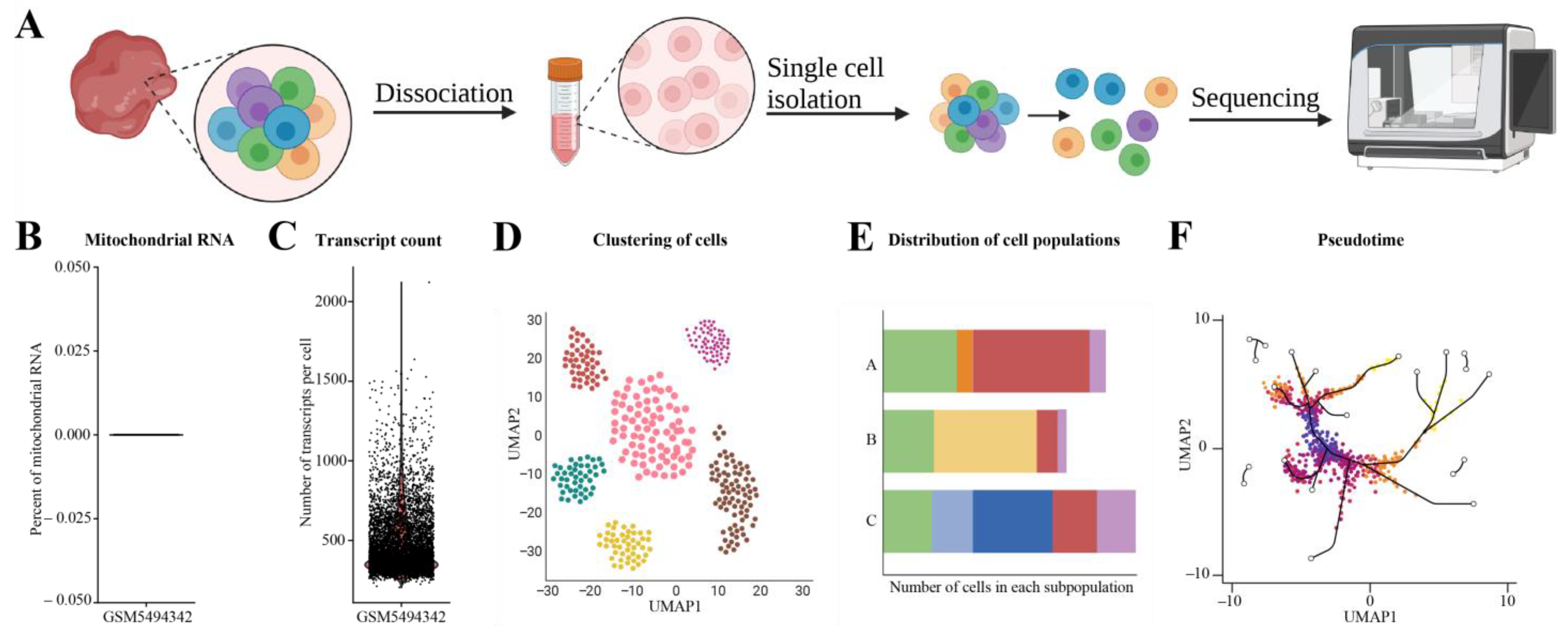
3.7. Single-Cell RNA-seq
4. Future Perspectives
4.1. Which Sequencing Technology Is Most Suitable for a Particular Experiment?
4.2. The Power of Metabolic Labeling
4.3. Selecting the Right Data Analysis Pipeline
Supplementary Materials
Author Contributions
Funding
Institutional Review Board Statement
Informed Consent Statement
Data Availability Statement
Acknowledgments
Conflicts of Interest
References
- Watson, J.D.; Crick, F.H. Molecular structure of nucleic acids; a structure for deoxyribose nucleic acid. Nature 1953, 171, 737–738. [Google Scholar] [CrossRef] [PubMed]
- Crick, F. Central dogma of molecular biology. Nature 1970, 227, 561–563. [Google Scholar] [CrossRef] [PubMed]
- Sanger, F.; Coulson, A.R. A rapid method for determining sequences in DNA by primed synthesis with DNA polymerase. J. Mol. Biol. 1975, 94, 441–448. [Google Scholar] [CrossRef] [PubMed]
- Maxam, A.M.; Gilbert, W. A new method for sequencing DNA. Proc. Natl. Acad. Sci. USA 1977, 74, 560–564. [Google Scholar] [CrossRef] [Green Version]
- Zimmermann, J.; Voss, H.; Schwager, C.; Stegemann, J.; Ansorge, W. Automated Sanger dideoxy sequencing reaction protocol. FEBS Lett. 1988, 233, 432–436. [Google Scholar] [CrossRef] [Green Version]
- International Human Genome Sequencing Consortium. Initial sequencing and analysis of the human genome. Nature 2001, 409, 860–921. [Google Scholar] [CrossRef] [Green Version]
- Schena, M.; Shalon, D.; Davis, R.W.; Brown, P.O. Quantitative monitoring of gene expression patterns with a complementary DNA microarray. Science 1995, 270, 467–470. [Google Scholar] [CrossRef] [Green Version]
- Clark, T.A.; Schweitzer, A.C.; Chen, T.X.; Staples, M.K.; Lu, G.; Wang, H.; Williams, A.; Blume, J.E. Discovery of tissue-specific exons using comprehensive human exon microarrays. Genome Biol. 2007, 8, R64. [Google Scholar] [CrossRef] [Green Version]
- Wang, Z.; Gerstein, M.; Snyder, M. RNA-Seq: A revolutionary tool for transcriptomics. Nat. Rev. Genet. 2009, 10, 57–63. [Google Scholar] [CrossRef]
- Ozsolak, F.; Milos, P.M. RNA sequencing: Advances, challenges and opportunities. Nat. Rev. Genet. 2011, 12, 87–98. [Google Scholar] [CrossRef]
- Schubert, M.; Lindgreen, S.; Orlando, L. AdapterRemoval v2: Rapid adapter trimming, identification, and read merging. BMC Res. Notes 2016, 9, 88. [Google Scholar] [CrossRef] [PubMed] [Green Version]
- Martin, M. Cutadapt removes adapter sequences from high-throughput sequencing reads. EMBnet. J. 2011, 17, 10–12. [Google Scholar] [CrossRef]
- Bolger, A.M.; Lohse, M.; Usadel, B. Trimmomatic: A flexible trimmer for Illumina sequence data. Bioinformatics 2014, 30, 2114–2120. [Google Scholar] [CrossRef] [Green Version]
- Chen, S.; Zhou, Y.; Chen, Y.; Gu, J. fastp: An ultra-fast all-in-one FASTQ preprocessor. Bioinformatics 2018, 34, i884–i890. [Google Scholar] [CrossRef]
- Li, H.; Handsaker, B.; Wysoker, A.; Fennell, T.; Ruan, J.; Homer, N.; Marth, G.; Abecasis, G.; Durbin, R.; Genome Project Data Processing Subgroup. The Sequence Alignment/Map format and SAMtools. Bioinformatics 2009, 25, 2078–2079. [Google Scholar] [CrossRef] [PubMed] [Green Version]
- Trapnell, C.; Pachter, L.; Salzberg, S.L. TopHat: Discovering splice junctions with RNA-Seq. Bioinformatics 2009, 25, 1105–1111. [Google Scholar] [CrossRef] [PubMed]
- Dobin, A.; Davis, C.A.; Schlesinger, F.; Drenkow, J.; Zaleski, C.; Jha, S.; Batut, P.; Chaisson, M.; Gingeras, T.R. STAR: Ultrafast universal RNA-seq aligner. Bioinformatics 2013, 29, 15–21. [Google Scholar] [CrossRef] [PubMed]
- Langmead, B.; Trapnell, C.; Pop, M.; Salzberg, S.L. Ultrafast and memory-efficient alignment of short DNA sequences to the human genome. Genome Biol. 2009, 10, R25. [Google Scholar] [CrossRef] [PubMed] [Green Version]
- Grabherr, M.G.; Haas, B.J.; Yassour, M.; Levin, J.Z.; Thompson, D.A.; Amit, I.; Adiconis, X.; Fan, L.; Raychowdhury, R.; Zeng, Q.; et al. Full-length transcriptome assembly from RNA-Seq data without a reference genome. Nat. Biotechnol. 2011, 29, 644–652. [Google Scholar] [CrossRef] [Green Version]
- Shen, S.; Park, J.W.; Lu, Z.X.; Lin, L.; Henry, M.D.; Wu, Y.N.; Zhou, Q.; Xing, Y. rMATS: Robust and flexible detection of differential alternative splicing from replicate RNA-Seq data. Proc. Natl. Acad. Sci. USA 2014, 111, E5593–E5601. [Google Scholar] [CrossRef] [Green Version]
- Jurges, C.; Dolken, L.; Erhard, F. Dissecting newly transcribed and old RNA using GRAND-SLAM. Bioinformatics 2018, 34, i218–i226. [Google Scholar] [CrossRef] [PubMed] [Green Version]
- Mortazavi, A.; Williams, B.A.; McCue, K.; Schaeffer, L.; Wold, B. Mapping and quantifying mammalian transcriptomes by RNA-Seq. Nat. Methods 2008, 5, 621–628. [Google Scholar] [CrossRef] [PubMed]
- Trapnell, C.; Williams, B.A.; Pertea, G.; Mortazavi, A.; Kwan, G.; van Baren, M.J.; Salzberg, S.L.; Wold, B.J.; Pachter, L. Transcript assembly and quantification by RNA-Seq reveals unannotated transcripts and isoform switching during cell differentiation. Nat. Biotechnol. 2010, 28, 511–515. [Google Scholar] [CrossRef] [PubMed] [Green Version]
- Anders, S.; Huber, W. Differential expression analysis for sequence count data. Genome Biol. 2010, 11, R106. [Google Scholar] [CrossRef] [Green Version]
- Robinson, M.D.; McCarthy, D.J.; Smyth, G.K. edgeR: A Bioconductor package for differential expression analysis of digital gene expression data. Bioinformatics 2010, 26, 139–140. [Google Scholar] [CrossRef] [Green Version]
- Liao, Y.; Smyth, G.K.; Shi, W. featureCounts: An efficient general purpose program for assigning sequence reads to genomic features. Bioinformatics 2014, 30, 923–930. [Google Scholar] [CrossRef] [Green Version]
- Di, Y.M.; Schafer, D.W.; Cumbie, J.S.; Chang, J.H. The NBP Negative Binomial Model for Assessing Differential Gene Expression from RNA-Seq. Stat. Appl. Genet. Mol. Biol. 2011, 10. [Google Scholar] [CrossRef]
- Auer, P.L.; Doerge, R.W. A Two-Stage Poisson Model for Testing RNA-Seq Data. Stat. Appl. Genet. Mol. 2011, 10. [Google Scholar] [CrossRef]
- Hardcastle, T.J.; Kelly, K.A. baySeq: Empirical Bayesian methods for identifying differential expression in sequence count data. BMC Bioinform. 2010, 11, 422. [Google Scholar] [CrossRef] [Green Version]
- Leng, N.; Dawson, J.A.; Thomson, J.A.; Ruotti, V.; Rissman, A.I.; Smits, B.M.G.; Haag, J.D.; Gould, M.N.; Stewart, R.M.; Kendziorski, C. EBSeq: An empirical Bayes hierarchical model for inference in RNA-seq experiments. Bioinformatics 2013, 29, 1035–1043. [Google Scholar] [CrossRef] [Green Version]
- Li, J.; Tibshirani, R. Finding consistent patterns: A nonparametric approach for identifying differential expression in RNA-Seq data. Stat. Methods Med. Res. 2013, 22, 519–536. [Google Scholar] [CrossRef] [PubMed] [Green Version]
- Van De Wiel, M.A.; Leday, G.G.; Pardo, L.; Rue, H.; Van Der Vaart, A.W.; Van Wieringen, W.N. Bayesian analysis of RNA sequencing data by estimating multiple shrinkage priors. Biostatistics 2013, 14, 113–128. [Google Scholar] [CrossRef] [PubMed] [Green Version]
- Itkonen, H.M.; Poulose, N.; Steele, R.E.; Martin, S.E.S.; Levine, Z.G.; Duveau, D.Y.; Carelli, R.; Singh, R.; Urbanucci, A.; Loda, M.; et al. Inhibition of O-GlcNAc Transferase Renders Prostate Cancer Cells Dependent on CDK9. Mol. Cancer Res. 2020, 18, 1512–1521. [Google Scholar] [CrossRef] [PubMed]
- Dennis, G., Jr.; Sherman, B.T.; Hosack, D.A.; Yang, J.; Gao, W.; Lane, H.C.; Lempicki, R.A. DAVID: Database for Annotation, Visualization, and Integrated Discovery. Genome Biol. 2003, 4, P3. [Google Scholar] [CrossRef] [PubMed] [Green Version]
- Chen, E.Y.; Tan, C.M.; Kou, Y.; Duan, Q.; Wang, Z.; Meirelles, G.V.; Clark, N.R.; Ma’ayan, A. Enrichr: Interactive and collaborative HTML5 gene list enrichment analysis tool. BMC Bioinform. 2013, 14, 128. [Google Scholar] [CrossRef] [Green Version]
- Bindea, G.; Mlecnik, B.; Hackl, H.; Charoentong, P.; Tosolini, M.; Kirilovsky, A.; Fridman, W.H.; Pages, F.; Trajanoski, Z.; Galon, J. ClueGO: A Cytoscape plug-in to decipher functionally grouped gene ontology and pathway annotation networks. Bioinformatics 2009, 25, 1091–1093. [Google Scholar] [CrossRef] [Green Version]
- Subramanian, A.; Tamayo, P.; Mootha, V.K.; Mukherjee, S.; Ebert, B.L.; Gillette, M.A.; Paulovich, A.; Pomeroy, S.L.; Golub, T.R.; Lander, E.S.; et al. Gene set enrichment analysis: A knowledge-based approach for interpreting genome-wide expression profiles. Proc. Natl. Acad. Sci. USA 2005, 102, 15545–15550. [Google Scholar] [CrossRef] [Green Version]
- Ietswaart, R.; Gyori, B.M.; Bachman, J.A.; Sorger, P.K.; Churchman, L.S. GeneWalk identifies relevant gene functions for a biological context using network representation learning. Genome Biol. 2021, 22, 55. [Google Scholar] [CrossRef]
- Hu, Q.; Poulose, N.; Girmay, S.; Heleva, A.; Doultsinos, D.; Gondane, A.; Steele, R.E.; Liu, X.; Loda, M.; Liu, S.; et al. Inhibition of CDK9 activity compromises global splicing in prostate cancer cells. RNA Biol. 2021, 18, 722–729. [Google Scholar] [CrossRef]
- Cleary, M.D.; Meiering, C.D.; Jan, E.; Guymon, R.; Boothroyd, J.C. Biosynthetic labeling of RNA with uracil phosphoribosyltransferase allows cell-specific microarray analysis of mRNA synthesis and decay. Nat. Biotechnol. 2005, 23, 232–237. [Google Scholar] [CrossRef]
- Core, L.J.; Waterfall, J.J.; Lis, J.T. Nascent RNA sequencing reveals widespread pausing and divergent initiation at human promoters. Science 2008, 322, 1845–1848. [Google Scholar] [CrossRef] [PubMed] [Green Version]
- Mahat, D.B.; Kwak, H.; Booth, G.T.; Jonkers, I.H.; Danko, C.G.; Patel, R.K.; Waters, C.T.; Munson, K.; Core, L.J.; Lis, J.T. Base-pair-resolution genome-wide mapping of active RNA polymerases using precision nuclear run-on (PRO-seq). Nat. Protoc. 2016, 11, 1455–1476. [Google Scholar] [CrossRef] [PubMed]
- Schwalb, B.; Michel, M.; Zacher, B.; Fruhauf, K.; Demel, C.; Tresch, A.; Gagneur, J.; Cramer, P. TT-seq maps the human transient transcriptome. Science 2016, 352, 1225–1228. [Google Scholar] [CrossRef] [PubMed]
- Herzog, V.A.; Reichholf, B.; Neumann, T.; Rescheneder, P.; Bhat, P.; Burkard, T.R.; Wlotzka, W.; von Haeseler, A.; Zuber, J.; Ameres, S.L. Thiol-linked alkylation of RNA to assess expression dynamics. Nat. Methods 2017, 14, 1198–1204. [Google Scholar] [CrossRef] [Green Version]
- Chae, M.; Danko, C.G.; Kraus, W.L. groHMM: A computational tool for identifying unannotated and cell type-specific transcription units from global run-on sequencing data. BMC Bioinform. 2015, 16, 222. [Google Scholar] [CrossRef] [Green Version]
- Duttke, S.H.; Chang, M.W.; Heinz, S.; Benner, C. Identification and dynamic quantification of regulatory elements using total RNA. Genome Res. 2019, 29, 1836–1846. [Google Scholar] [CrossRef]
- Nagari, A.; Murakami, S.; Malladi, V.S.; Kraus, W.L. Computational Approaches for Mining GRO-Seq Data to Identify and Characterize Active Enhancers. Methods Mol. Biol. 2017, 1468, 121–138. [Google Scholar] [CrossRef] [Green Version]
- Neumann, T.; Herzog, V.A.; Muhar, M.; von Haeseler, A.; Zuber, J.; Ameres, S.L.; Rescheneder, P. Quantification of experimentally induced nucleotide conversions in high-throughput sequencing datasets. BMC Bioinform. 2019, 20, 258. [Google Scholar] [CrossRef] [Green Version]
- Marasco, L.E.; Kornblihtt, A.R. The physiology of alternative splicing. Nat. Rev. Mol. Cell Biol. 2022. [Google Scholar] [CrossRef]
- Katz, Y.; Wang, E.T.; Airoldi, E.M.; Burge, C.B. Analysis and design of RNA sequencing experiments for identifying isoform regulation. Nat. Methods 2010, 7, 1009–1015. [Google Scholar] [CrossRef]
- Alamancos, G.P.; Pages, A.; Trincado, J.L.; Bellora, N.; Eyras, E. Leveraging transcript quantification for fast computation of alternative splicing profiles. RNA 2015, 21, 1521–1531. [Google Scholar] [CrossRef] [PubMed] [Green Version]
- Kakaradov, B.; Xiong, H.Y.; Lee, L.J.; Jojic, N.; Frey, B.J. Challenges in estimating percent inclusion of alternatively spliced junctions from RNA-seq data. BMC Bioinform. 2012, 13 (Suppl. S6), S11. [Google Scholar] [CrossRef] [PubMed] [Green Version]
- Tang, F.; Barbacioru, C.; Wang, Y.; Nordman, E.; Lee, C.; Xu, N.; Wang, X.; Bodeau, J.; Tuch, B.B.; Siddiqui, A.; et al. mRNA-Seq whole-transcriptome analysis of a single cell. Nat. Methods 2009, 6, 377–382. [Google Scholar] [CrossRef] [PubMed]
- Satija, R.; Farrell, J.A.; Gennert, D.; Schier, A.F.; Regev, A. Spatial reconstruction of single-cell gene expression data. Nat. Biotechnol. 2015, 33, 495–502. [Google Scholar] [CrossRef] [PubMed] [Green Version]
- Zhang, Y.; Park, C.; Bennett, C.; Thornton, M.; Kim, D. Rapid and accurate alignment of nucleotide conversion sequencing reads with HISAT-3N. Genome Res. 2021, 31, 1290–1295. [Google Scholar] [CrossRef]
- Trapnell, C.; Roberts, A.; Goff, L.; Pertea, G.; Kim, D.; Kelley, D.R.; Pimentel, H.; Salzberg, S.L.; Rinn, J.L.; Pachter, L. Differential gene and transcript expression analysis of RNA-seq experiments with TopHat and Cufflinks. Nat. Protoc. 2012, 7, 562–578. [Google Scholar] [CrossRef] [Green Version]
- Haas, B.J.; Dobin, A.; Li, B.; Stransky, N.; Pochet, N.; Regev, A. Accuracy assessment of fusion transcript detection via read-mapping and de novo fusion transcript assembly-based methods. Genome Biol. 2019, 20, 213. [Google Scholar] [CrossRef] [Green Version]
- Dorney, R.; Dhungel, B.P.; Rasko, J.E.J.; Hebbard, L.; Schmitz, U. Recent advances in cancer fusion transcript detection. Brief. Bioinform. 2023, 24, bbac519. [Google Scholar] [CrossRef]
- Chen, Y.; Wang, Y.; Chen, W.; Tan, Z.; Song, Y.; Human Genome Structural Variation, C.; Chen, H.; Chong, Z. Gene Fusion Detection and Characterization in Long-Read Cancer Transcriptome Sequencing Data with FusionSeeker. Cancer Res. 2023, 83, 28–33. [Google Scholar] [CrossRef]
- Ramanathan, M.; Porter, D.F.; Khavari, P.A. Methods to study RNA-protein interactions. Nat. Methods 2019, 16, 225–234. [Google Scholar] [CrossRef]
- Erhard, F.; Baptista, M.A.P.; Krammer, T.; Hennig, T.; Lange, M.; Arampatzi, P.; Jurges, C.S.; Theis, F.J.; Saliba, A.E.; Dolken, L. scSLAM-seq reveals core features of transcription dynamics in single cells. Nature 2019, 571, 419–423. [Google Scholar] [CrossRef] [PubMed]
- Holler, K.; Neuschulz, A.; Drewe-Boss, P.; Mintcheva, J.; Spanjaard, B.; Arsie, R.; Ohler, U.; Landthaler, M.; Junker, J.P. Spatio-temporal mRNA tracking in the early zebrafish embryo. Nat. Commun. 2021, 12, 3358. [Google Scholar] [CrossRef] [PubMed]


| Technique | Description | Advantages | Limitations |
|---|---|---|---|
| Standard RNA-seq | Quantifies the levels of RNA from a biological sample at a given moment. |
|
|
| Nascent RNA-seq | Nucleotide analogue based techniques used to assess RNA synthesis. The nascent RNAs incorporate the nucleotide analogue and are either enriched using affinity-based techniques or decoded computationally. |
|
|
| scRNA-seq | Measures the gene expression levels at single cell resolution. |
|
|
| Technique | Advantages/Comments | Limitations |
|---|---|---|
| Analysis of 2,4-dithiouracil labeled and enriched RNA using a microarray [40]. Description: the labeled RNA is biotinylated and enriched using streptavidin beads. The isolated RNA is analyzed using a microarray. |
|
|
| GRO-seq (global run-on sequencing [41]). Description: labeled nucleotides (Br-UTP), are incorporated into the RNA. The RNA is then hydrolyzed and purified using antibody-coated beads. |
|
|
| PRO-seq (precision nuclear run-on sequencing [42]). Description: biotinylated NTPs are incorporated into the nascent mRNA, inhibiting transcription. 3′ end sequencing reveals the precise location of the stalled RNA polymerase. |
|
|
| TT-seq [43] (Transient transcriptome sequencing). Description: label with 4-thiouridine, isolate RNA, fragment RNA, biotinylate and purify the labeled RNA, and sequence. |
|
|
| SLAM-seq (Thiol (SH)-linked alkylation for the metabolic sequencing of RNA [44]). Description: labeling with 4-thiouridine, followed by alkylation which allows the nucleotide analog to be recognized as a cytosine. To measure the nascent mRNA synthesis the T > C conversion is measured. |
|
|
Disclaimer/Publisher’s Note: The statements, opinions and data contained in all publications are solely those of the individual author(s) and contributor(s) and not of MDPI and/or the editor(s). MDPI and/or the editor(s) disclaim responsibility for any injury to people or property resulting from any ideas, methods, instructions or products referred to in the content. |
© 2023 by the authors. Licensee MDPI, Basel, Switzerland. This article is an open access article distributed under the terms and conditions of the Creative Commons Attribution (CC BY) license (https://creativecommons.org/licenses/by/4.0/).
Share and Cite
Gondane, A.; Itkonen, H.M. Revealing the History and Mystery of RNA-Seq. Curr. Issues Mol. Biol. 2023, 45, 1860-1874. https://doi.org/10.3390/cimb45030120
Gondane A, Itkonen HM. Revealing the History and Mystery of RNA-Seq. Current Issues in Molecular Biology. 2023; 45(3):1860-1874. https://doi.org/10.3390/cimb45030120
Chicago/Turabian StyleGondane, Aishwarya, and Harri M. Itkonen. 2023. "Revealing the History and Mystery of RNA-Seq" Current Issues in Molecular Biology 45, no. 3: 1860-1874. https://doi.org/10.3390/cimb45030120