
Frequency-Domain-Based Structure Losses for CycleGAN-Based Cone-Beam Computed Tomography Translation

 , , , , and
Abstract
:1. Introduction
- 1.
- Our proposed frequency structure loss operates in the frequency domain, enforcing constraints where spatial correspondences between images are less sensitive, allowing it to be used effectively on unpaired data.
- 2.
- The frequency structure loss improves performance over the baseline CycleGAN and provides images that are more robust than existing methods.
- 3.
- The calculation of our loss is faster and less resource-intensive compared to similar losses, such as in Yang et al. [25].
- 4.
- Our loss is generalized and does not need any data-dependent configuration, enabling its use for a range of use cases.
2. Materials and Methods
2.1. Model Architecture
2.1.1. Image-to-Image Translation Using GANs
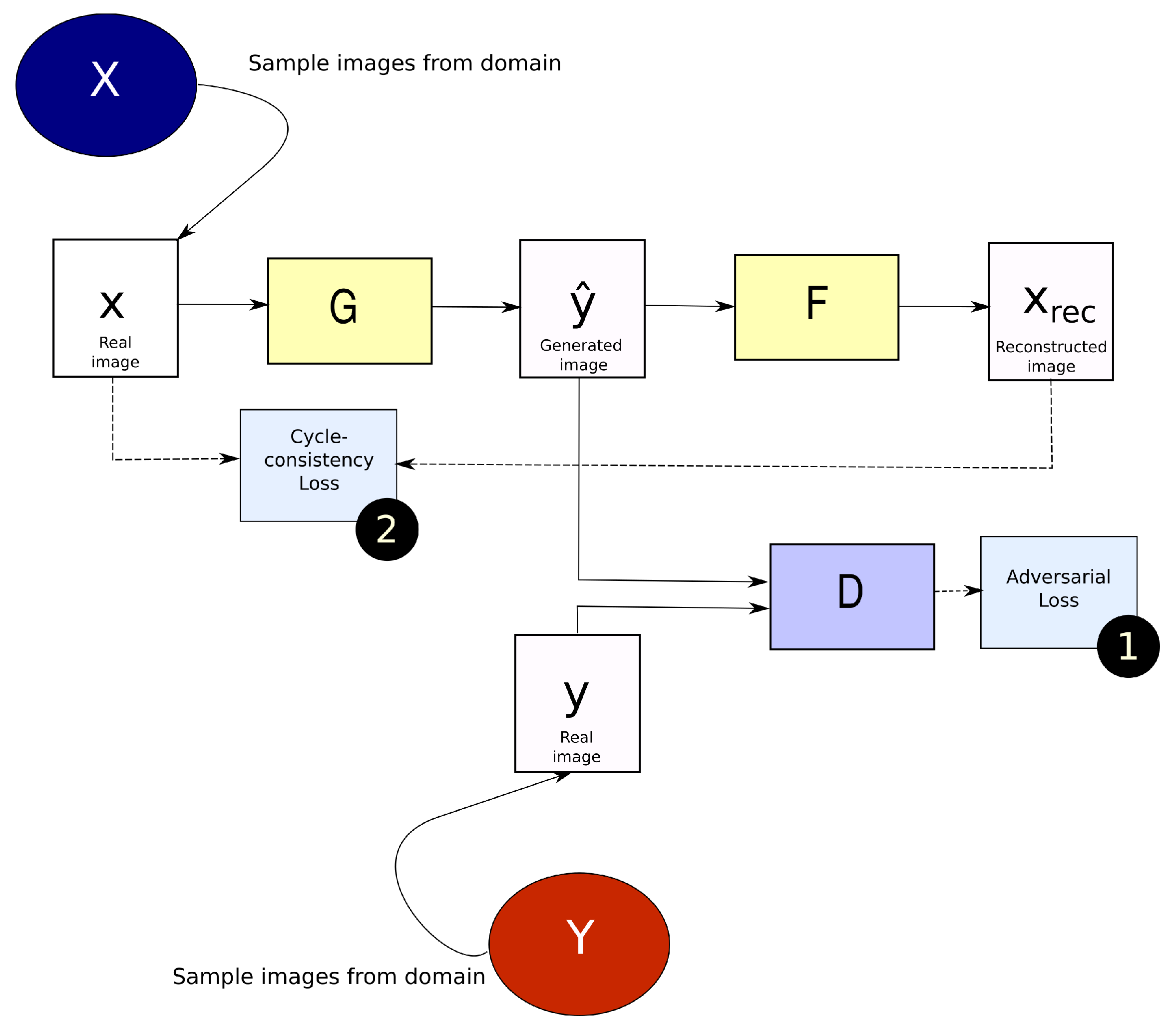
2.1.2. CycleGAN
2.2. Generalized Frequency Loss
2.3. Evaluation
2.3.1. Image Similarity Metrics
- Mean absolute error (MAE)where total number of voxels in the image. , in our work, is the CT image while , is the generated image.
- Mean squared error (MSE)The MSE largely penalizes deviations from the reference image due to the difference being squared.
- Normalized mean squared error (NMSE)The gives the mean squared error while also factoring in the signal power.
- Power-to-signal-noise ratio (PSNR)refers to the maximum value of the image. is computed as described in Equation (12).
- Structural similarity index metric (SSIM)is computed using the formula presented below, with denoted as x, and as y.where and represent the mean and variance respectively. and are variables used to stabilize division.
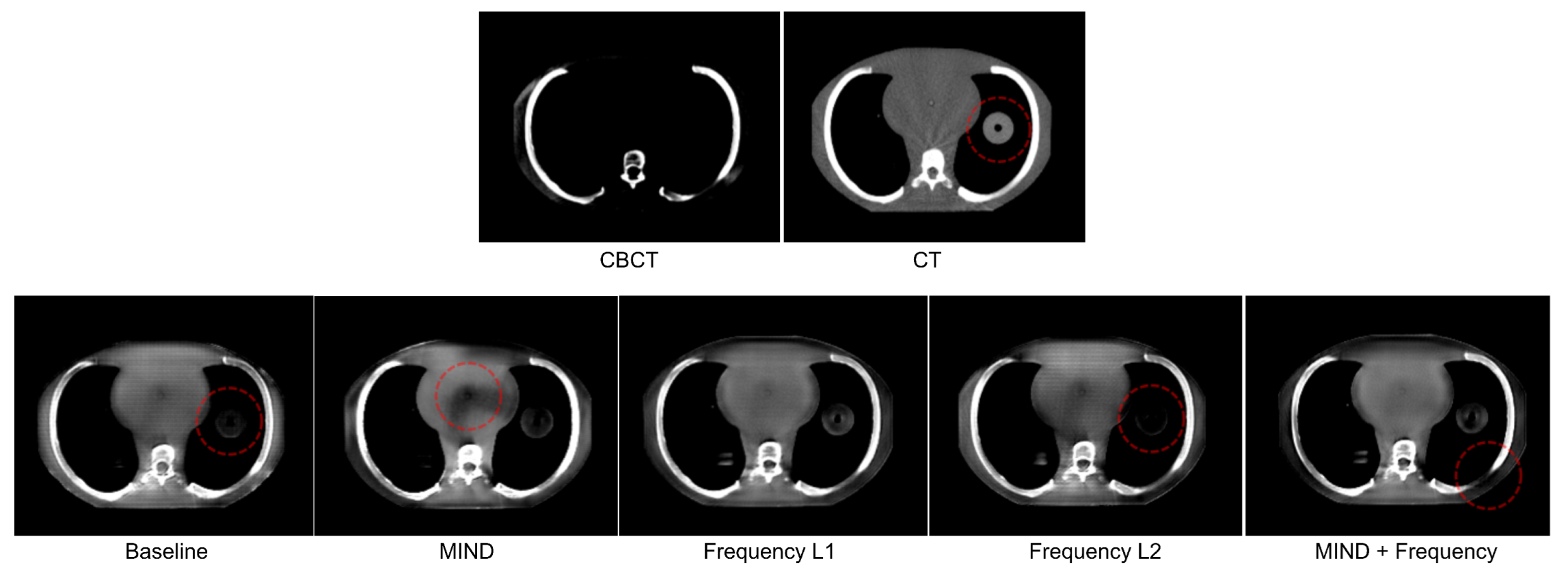
2.3.2. Qualitative Inspection
- 1.
- Presence of artifacts or undesirable elements: The induction of artifacts is an established drawback of GAN-based generative models [30]. Such artifacts are hard to identify using pixel-based quantitative metrics and, to the best of our knowledge, no other metric that fully captures the range of possible artifacts in a CycleGAN is available. To this end, we inspect images manually to check for artifacts or any undesirable elements such as localized checkerboard artifacts that may appear randomly.
- 2.
- Quality of image in terms of clarity: This criterion aims to identify the reduction in perceived image quality for translated images. Some very commonly seen phenomena in CycleGAN translations are blurring, aliasing-like effects, and bright spots in parts of the image. Ideally, a reader study would be performed to analyze these factors. However, that is beyond the scope of this study.
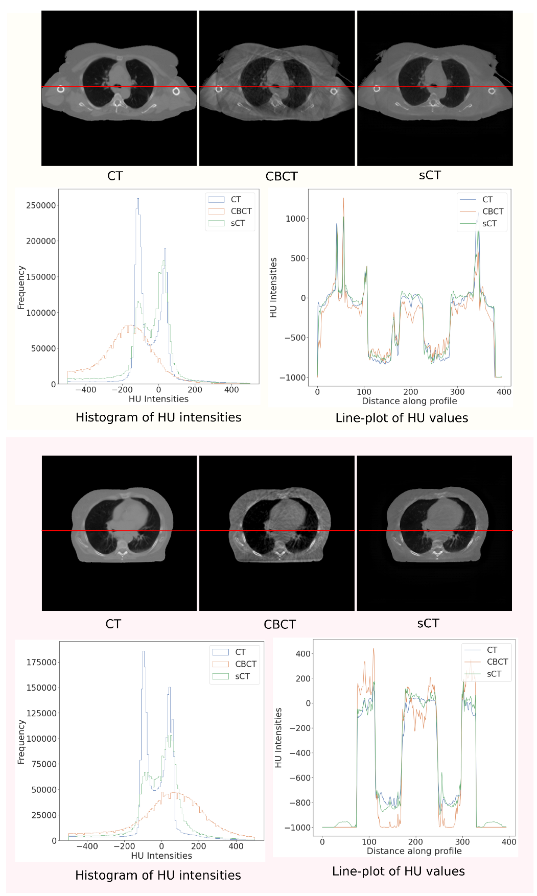
2.3.3. Out-of-Distribution Analysis
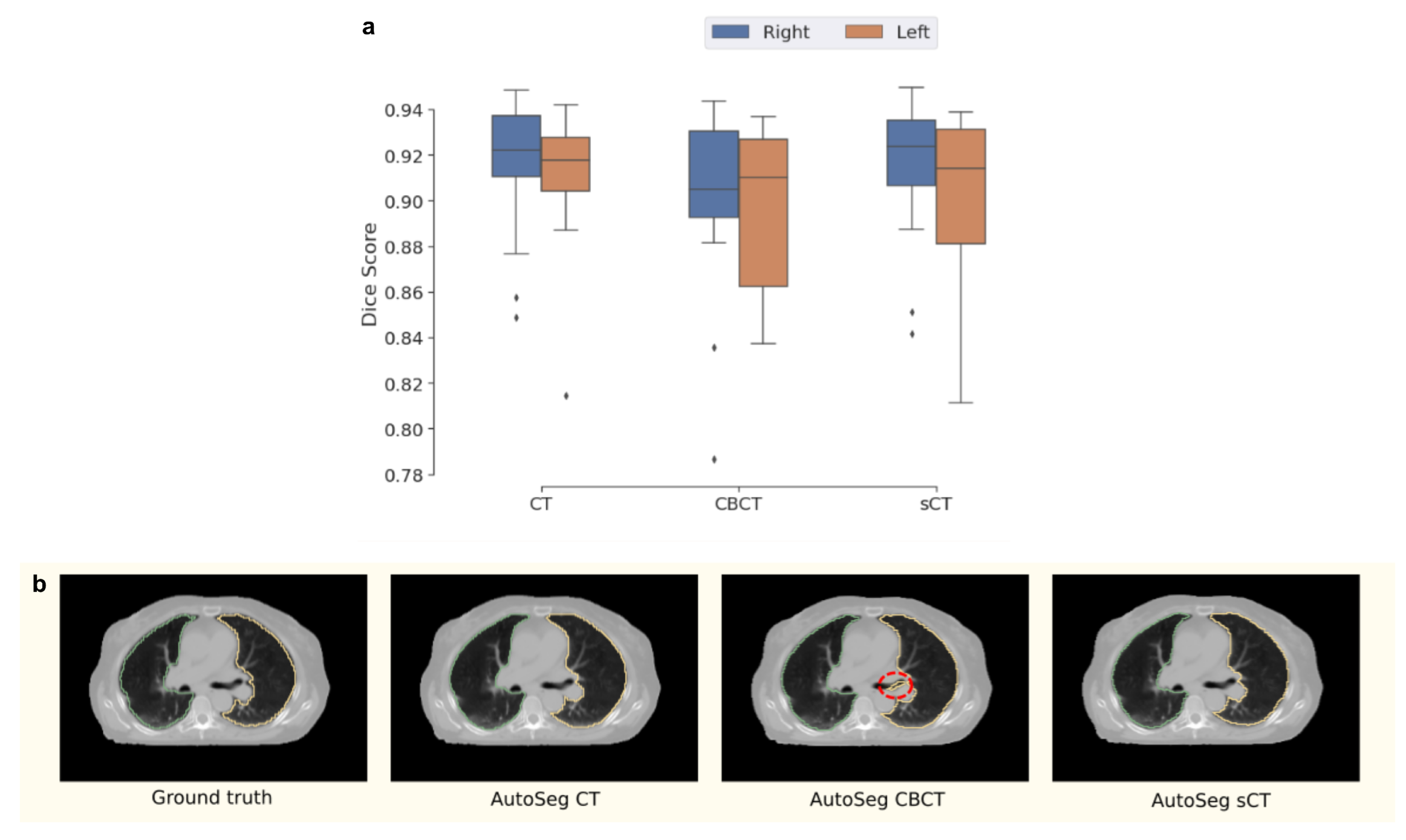
2.3.4. Domain-Specific Evaluation
3. Experiments
3.1. Datasets
3.2. Data Pre-Processing
- 1.
- Obtain frequency counts of spacing of all scans in the dataset.
- 2.
- Sort spacings in ascending order and rank all spacings based on their frequency counts.
- 3.
- Select the smallest rank starting from the bottom of the list.
Data Stratification for Modeling
- 1.
- Select the rescanned CT and the CBCT with the smallest time differences between them (delta). The maximum time difference between the two is limited to one day so that scans with potentially larger anatomical changes are ignored.
- 2.
- The rescanned CT is registered to the CBCT through deformable registration using parameters from the SimpleElastix library. Parameter files are available at https://github.com/Maastro-CDS-Imaging-Group/clinical-evaluation/tree/master/configs, accessed on 13 May 2021 [35].
- 3.
- Apply the registration transform to the rescanned CT and available contours (only available on the test set).
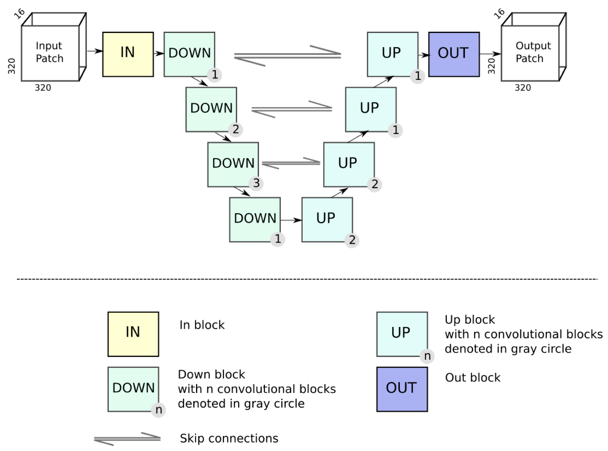
3.3. Network Configuration
3.4. Experimental Setup
- 1.
- Baseline CycleGAN: The original CycleGAN implementation [17] without any additional structural constraints added.
- 2.
- MIND loss: The MIND loss [25] was added as a structural constraint consistent with the authors’ proposed implementation. However, two changes were introduced in the experiment configuration for the MIND loss. In the original work, authors propose a weight of . In our experiments, this is changed to through scale-matching with other losses. Additionally, a patch size of is used for the MIND loss due to memory restrictions.
- 3.
- Generalized frequency loss: Our proposed loss was added as a structural constraint to the CycleGAN as outlined in Section 2.2. Two different distance metrics were tested for generalized frequency loss, shown in Equation (9),
- (a)
- distance between the frequency representations;
- (b)
- distance between the frequency representations.
Other distance metrics such as distances may also offer interesting properties but they are not considered in this study. - 4.
- Combined Loss: A combination of Frequency loss and the MIND loss is investigated as well. The losses have values consistent with their individual experiments, and are summed to obtain the combined loss. This is trained with a patch size of .
4. Results
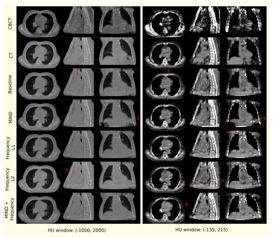
- 1.
- Air pockets that are present in the original scan are closed by the baseline model.
- 2.
- For the baseline model, a decrease in the quality of the translated image is observed through the addition of checkerboard-like patterns.
- 3.
- MIND loss adds unexplained artifacts in the form of black density reduction fields.
- 4.
- Frequency also closes air pockets similar to the baseline model.
- 5.
- Frequency provides a shift in density as we move down to the diaphragm, as observed on the sagittal view.
- 6.
- MIND + Frequency causes a random drop in density across a particular region.
4.1. Out-of-Distribution Evaluation
4.2. Domain-Specific Evaluation
5. Discussion
6. Conclusions
Author Contributions
Funding
Institutional Review Board Statement
Informed Consent Statement
Data Availability Statement
Acknowledgments
Conflicts of Interest
Appendix A

References
- Schulze, R.; Heil, U.; Groβ, D.; Bruellmann, D.D.; Dranischnikow, E.; Schwanecke, U.; Schoemer, E. Artefacts in CBCT: A review. Dentomaxillofac. Radiol. 2011, 40, 265–273. [Google Scholar] [CrossRef] [PubMed] [Green Version]
- Lechuga, L.; Weidlich, G.A. Cone Beam CT vs. Fan Beam CT: A Comparison of Image Quality and Dose Delivered Between Two Differing CT Imaging Modalities. Cureus 2016, 8, e778. [Google Scholar] [CrossRef] [PubMed] [Green Version]
- Jin, J.Y.; Ren, L.; Liu, Q.; Kim, J.; Wen, N.; Guan, H.; Movsas, B.; Chetty, I.J. Combining scatter reduction and correction to improve image quality in cone-beam computed tomography (CBCT). Med. Phys. 2010, 37, 5634–5644. [Google Scholar] [CrossRef] [PubMed]
- Dunlop, A.; McQuaid, D.; Nill, S.; Murray, J.; Poludniowski, G.; Hansen, V.N.; Bhide, S.; Nutting, C.; Harrington, K.; Newbold, K.; et al. Vergleich unterschiedlicher CT-Kalibrierungsmethoden zur Dosisberechnung auf Basis der Kegelstrahlcomputertomographie. Strahlenther. Und Onkol. 2015, 191, 970–978. [Google Scholar] [CrossRef] [PubMed] [Green Version]
- Landry, G.; Nijhuis, R.; Dedes, G.; Handrack, J.; Thieke, C.; Janssens, G.; de Xivry, J.; Reiner, M.; Kamp, F.; Wilkens, J.J.; et al. Investigating CT to CBCT image registration for head and neck proton therapy as a tool for daily dose recalculation. Med. Phys. 2015, 42, 1354–1366. [Google Scholar] [CrossRef]
- Zhao, W.; Vernekohl, D.; Zhu, J.; Wang, L.; Xing, L. A model-based scatter artifacts correction for cone beam CT. Med. Phys. 2016, 43, 1736–1753. [Google Scholar] [CrossRef] [Green Version]
- Ronneberger, O.; Fischer, P.; Brox, T. U-net: Convolutional networks for biomedical image segmentation. In Proceedings of the International Conference on Medical Image Computing and Computer-Assisted Intervention, Munich, Germany, 5–9 October 2015; pp. 234–241. [Google Scholar]
- Kida, S.; Nakamoto, T.; Nakano, M.; Nawa, K.; Haga, A.; Kotoku, J.; Yamashita, H.; Nakagawa, K. Cone Beam Computed Tomography Image Quality Improvement Using a Deep Convolutional Neural Network. Cureus 2018, 10, e2548. [Google Scholar] [CrossRef] [Green Version]
- Landry, G.; Hansen, D.; Kamp, F.; Li, M.; Hoyle, B.; Weller, J.; Parodi, K.; Belka, C.; Kurz, C. Corrigendum: Comparing Unet training with three different datasets to correct CBCT images for prostate radiotherapy dose calculations. Phys. Med. Biol. 2019, 64, 035011. [Google Scholar] [CrossRef]
- Yuan, N.; Dyer, B.; Rao, S.; Chen, Q.; Benedict, S.; Shang, L.; Kang, Y.; Qi, J.; Rong, Y. Convolutional neural network enhancement of fast-scan low-dose cone-beam CT images for head and neck radiotherapy. Phys. Med. Biol. 2020, 65, 035003. [Google Scholar] [CrossRef]
- Thummerer, A.; Zaffino, P.; Meijers, A.; Marmitt, G.G.; Seco, J.; Steenbakkers, R.J.; Langendijk, J.A.; Both, S.; Spadea, M.F.; Knopf, A.C. Comparison of CBCT based synthetic CT methods suitable for proton dose calculations in adaptive proton therapy. Phys. Med. Biol. 2020, 65, 095002. [Google Scholar] [CrossRef]
- Wang, Z.; Bovik, A.C.; Sheikh, H.R.; Simoncelli, E.P. Image quality assessment: From error visibility to structural similarity. IEEE Trans. Image Process. 2004, 13, 600–612. [Google Scholar] [CrossRef] [Green Version]
- Isola, P.; Zhu, J.Y.; Zhou, T.; Efros, A.A. Image-To-Image Translation With Conditional Adversarial Networks. In Proceedings of the IEEE Conference on Computer Vision and Pattern Recognition (CVPR), Honolulu, HI, USA, 21–26 July 2017. [Google Scholar]
- Zhang, Y.; Yue, N.; Su, M.Y.; Liu, B.; Ding, Y.; Zhou, Y.; Wang, H.; Kuang, Y.; Nie, K. Improving CBCT quality to CT level using deep learning with generative adversarial network. Med. Phys. 2021, 48, 2816–2826. [Google Scholar] [CrossRef]
- Dahiya, N.; Alam, S.R.; Zhang, P.; Zhang, S.Y.; Li, T.; Yezzi, A.; Nadeem, S. Multitask 3D CBCT-to-CT translation and organs-at-risk segmentation using physics-based data augmentation. Med. Phys. 2021, 48, 5130–5141. [Google Scholar] [CrossRef]
- Tang, B.; Wu, F.; Fu, Y.; Wang, X.; Wang, P.; Orlandini, L.C.; Li, J.; Hou, Q. Dosimetric evaluation of synthetic CT image generated using a neural network for MR-only brain radiotherapy. J. Appl. Clin. Med. Phys. 2021, 22, 55–62. [Google Scholar] [CrossRef]
- Zhu, J.Y.; Park, T.; Isola, P.; Efros, A.A. Unpaired Image-to-Image Translation Using Cycle-Consistent Adversarial Networks. In Proceedings of the IEEE International Conference on Computer Vision, Venice, Italy, 22–29 October 2017; Volume 2017, pp. 2242–2251. [Google Scholar] [CrossRef] [Green Version]
- Kurz, C.; Maspero, M.; Savenije, M.H.; Landry, G.; Kamp, F.; Pinto, M.; Li, M.; Parodi, K.; Belka, C.; Van Den Berg, C.A. CBCT correction using a cycle-consistent generative adversarial network and unpaired training to enable photon and proton dose calculation. Phys. Med. Biol. 2019, 64, 225004. [Google Scholar] [CrossRef]
- Maspero, M.; Houweling, A.C.; Savenije, M.H.; van Heijst, T.C.; Verhoeff, J.J.; Kotte, A.N.; van den Berg, C.A. A single neural network for cone-beam computed tomography-based radiotherapy of head-and-neck, lung and breast cancer. Phys. Imaging Radiat. Oncol. 2020, 14, 24–31. [Google Scholar] [CrossRef]
- Liu, Y.; Lei, Y.; Wang, T.; Fu, Y.; Tang, X.; Curran, W.J.; Liu, T.; Patel, P.; Yang, X. CBCT-based synthetic CT generation using deep-attention cycleGAN for pancreatic adaptive radiotherapy. Med. Phys. 2020, 47, 2472–2483. [Google Scholar] [CrossRef]
- Harms, J.; Lei, Y.; Wang, T.; Zhang, R.; Zhou, J.; Tang, X.; Curran, W.J.; Liu, T.; Yang, X. Paired cycle-GAN-based image correction for quantitative cone-beam computed tomography. Med. Phys. 2019, 46, 3998–4009. [Google Scholar] [CrossRef]
- Eckl, M.; Hoppen, L.; Sarria, G.R.; Boda-Heggemann, J.; Simeonova-Chergou, A.; Steil, V.; Giordano, F.A.; Fleckenstein, J. Evaluation of a cycle-generative adversarial network-based cone-beam CT to synthetic CT conversion algorithm for adaptive radiation therapy. Phys. Medica 2020, 80, 308–316. [Google Scholar] [CrossRef]
- Kida, S.; Kaji, S.; Nawa, K.; Imae, T.; Nakamoto, T.; Ozaki, S.; Ohta, T.; Nozawa, Y.; Nakagawa, K. Visual enhancement of Cone-beam CT by use of CycleGAN. Med. Phys. 2020, 47, 998–1010. [Google Scholar] [CrossRef]
- Shrivastava, A.; Pfister, T.; Tuzel, O.; Susskind, J.; Wang, W.; Webb, R. Learning from simulated and unsupervised images through adversarial training. In Proceedings of the IEEE Conference on Computer Vision and Pattern Recognition, Honolulu, HI, USA, 21–26 July 2017; pp. 2107–2116. [Google Scholar]
- Yang, H.; Sun, J.; Carass, A.; Zhao, C.; Lee, J.; Xu, Z.; Prince, J. Unpaired brain MR-to-CT synthesis using a structure-constrained CycleGAN. In Deep Learning in Medical Image Analysis and Multimodal Learning for Clinical Decision Support; Springer: Berlin/Heidelberg, Germany, 2018; pp. 174–182. [Google Scholar]
- Jiang, L.; Dai, B.; Wu, W.; Loy, C.C. Focal frequency loss for image reconstruction and synthesis. In Proceedings of the IEEE/CVF International Conference on Computer Vision, Montreal, QC, Canada, 10–17 October 2021; pp. 13919–13929. [Google Scholar]
- Goodfellow, I.; Pouget-Abadie, J.; Mirza, M.; Xu, B.; Warde-Farley, D.; Ozair, S.; Courville, A.; Bengio, Y. Generative adversarial networks. Commun. ACM 2020, 63, 139–144. [Google Scholar] [CrossRef]
- Mirza, M.; Osindero, S. Conditional Generative Adversarial Nets. arXiv 2014, arXiv:1411.1784. [Google Scholar]
- Chow, L.S.; Paramesran, R. Review of medical image quality assessment. Biomed. Signal Process. Control 2016, 27, 145–154. [Google Scholar] [CrossRef]
- Zhang, X.; Karaman, S.; Chang, S.F. Detecting and Simulating Artifacts in GAN Fake Images. In Proceedings of the 2019 IEEE International Workshop on Information Forensics and Security (WIFS), Delft, The Netherlands, 9–12 December 2019; pp. 1–6. [Google Scholar] [CrossRef] [Green Version]
- Hofmanninger, J.; Prayer, F.; Pan, J.; Röhrich, S.; Prosch, H.; Langs, G. Automatic lung segmentation in routine imaging is primarily a data diversity problem, not a methodology problem. Eur. Radiol. Exp. 2020, 4, 50. [Google Scholar] [CrossRef]
- Hadzic, I.; Pai, S.; Rao, C.; Teuwen, J. Ganslate-Team/Ganslate: A Simple and Extensible Gan Image-to-Image Translation Framework. 2021. Available online: https://doi.org/10.5281/zenodo.5494572 (accessed on 8 September 2021). [CrossRef]
- Judy, P.F.; Balter, S.; Bassano, D.; McCullough, E.C.; Payne, J.T.; Rothenberg, L. Phantoms for Performance Evaluation and Quality Assurance of CT Scanners; Report No. 1. 1977, Diagnostic Radiology Committee Task Force on CT Scanner Phantoms; American Association of Physicists in Medicine: Alexandria, VA, USA, 1977; ISBN 978-1-888340-04-4. [Google Scholar] [CrossRef]
- Lowekamp, B.; Chen, D.; Ibanez, L.; Blezek, D. The Design of SimpleITK. Front. Neuroinform. 2013, 7, 45. [Google Scholar] [CrossRef] [Green Version]
- Marstal, K.; Berendsen, F.; Staring, M.; Klein, S. SimpleElastix: A User-Friendly, Multi-lingual Library for Medical Image Registration. In Proceedings of the 2016 IEEE Conference on Computer Vision and Pattern Recognition Workshops (CVPRW), Las Vegas, NV, USA, 26 June–1 July 2016; pp. 574–582. [Google Scholar] [CrossRef]
- Milletari, F.; Navab, N.; Ahmadi, S.A. V-net: Fully convolutional neural networks for volumetric medical image segmentation. In Proceedings of the 2016 fourth international conference on 3D vision (3DV), Stanford, CA, USA, 25–28 October 2016; pp. 565–571. [Google Scholar]
- Gragnaniello, D.; Cozzolino, D.; Marra, F.; Poggi, G.; Verdoliva, L. Are GAN generated images easy to detect? A critical analysis of the state-of-the-art. arXiv 2021, arXiv:2104.02617. [Google Scholar]


| Generator | VNet 3D |
| Discriminator | PatchGAN 3D |
| Learning rate | D: 0.0002, G: 0.0004 |
| Batch size | 1 |
| LR schedule | Fixed for 50%, Linear decay for 50% |
| Optimizer | Adam |
| Lambda () | 5 |
| Input size (z, x, y) | |
| Normalization | Instance normalization |
| Training iterations | 30,000 |
| Model | MAE | MSE | NMSE | PSNR | SSIM |
|---|---|---|---|---|---|
| Baseline | 88.85 | 24,244 | 0.031 | 29.37 | 0.935 |
| MIND | 85.91 | 25,604 | 0.032 | 29.27 | 0.944 |
| Frequency loss | 85.50 | 20,433 | 0.026 | 30.02 | 0.935 |
| Frequency loss | 85.97 | 20,247 | 0.027 | 30.12 | 0.938 |
| MIND + Frequency loss | 86.63 | 21,125 | 0.027 | 29.88 | 0.935 |
| Model | MAE | MSE | NMSE | PSNR | SSIM |
|---|---|---|---|---|---|
| Baseline | 72.16 | 16207 | 0.024 | 34.55 | 0.976 |
| MIND | 62.74 | 11,303 | 0.017 | 36.12 | 0.985 |
| Frequency loss | 71.39 | 16,878 | 0.025 | 34.38 | 0.976 |
| Frequency loss | 63.65 | 12,046 | 0.018 | 35.84 | 0.983 |
| MIND + Frequency loss | 75.34 | 17,723 | 0.027 | 34.16 | 0.975 |
| Left Lung | Right Lung | |
|---|---|---|
| CT | 0.910 | 0.913 |
| CBCT | 0.898 | 0.902 |
| sCT | 0.900 | 0.915 |
Disclaimer/Publisher’s Note: The statements, opinions and data contained in all publications are solely those of the individual author(s) and contributor(s) and not of MDPI and/or the editor(s). MDPI and/or the editor(s) disclaim responsibility for any injury to people or property resulting from any ideas, methods, instructions or products referred to in the content. |
© 2023 by the authors. Licensee MDPI, Basel, Switzerland. This article is an open access article distributed under the terms and conditions of the Creative Commons Attribution (CC BY) license (https://creativecommons.org/licenses/by/4.0/).
Share and Cite
Pai, S.; Hadzic, I.; Rao, C.; Zhovannik, I.; Dekker, A.; Traverso, A.; Asteriadis, S.; Hortal, E. Frequency-Domain-Based Structure Losses for CycleGAN-Based Cone-Beam Computed Tomography Translation. Sensors 2023, 23, 1089. https://doi.org/10.3390/s23031089
Pai S, Hadzic I, Rao C, Zhovannik I, Dekker A, Traverso A, Asteriadis S, Hortal E. Frequency-Domain-Based Structure Losses for CycleGAN-Based Cone-Beam Computed Tomography Translation. Sensors. 2023; 23(3):1089. https://doi.org/10.3390/s23031089
Chicago/Turabian StylePai, Suraj, Ibrahim Hadzic, Chinmay Rao, Ivan Zhovannik, Andre Dekker, Alberto Traverso, Stylianos Asteriadis, and Enrique Hortal. 2023. "Frequency-Domain-Based Structure Losses for CycleGAN-Based Cone-Beam Computed Tomography Translation" Sensors 23, no. 3: 1089. https://doi.org/10.3390/s23031089