
Online Activity Recognition Combining Dynamic Segmentation and Emergent Modeling


Abstract
:1. Introduction
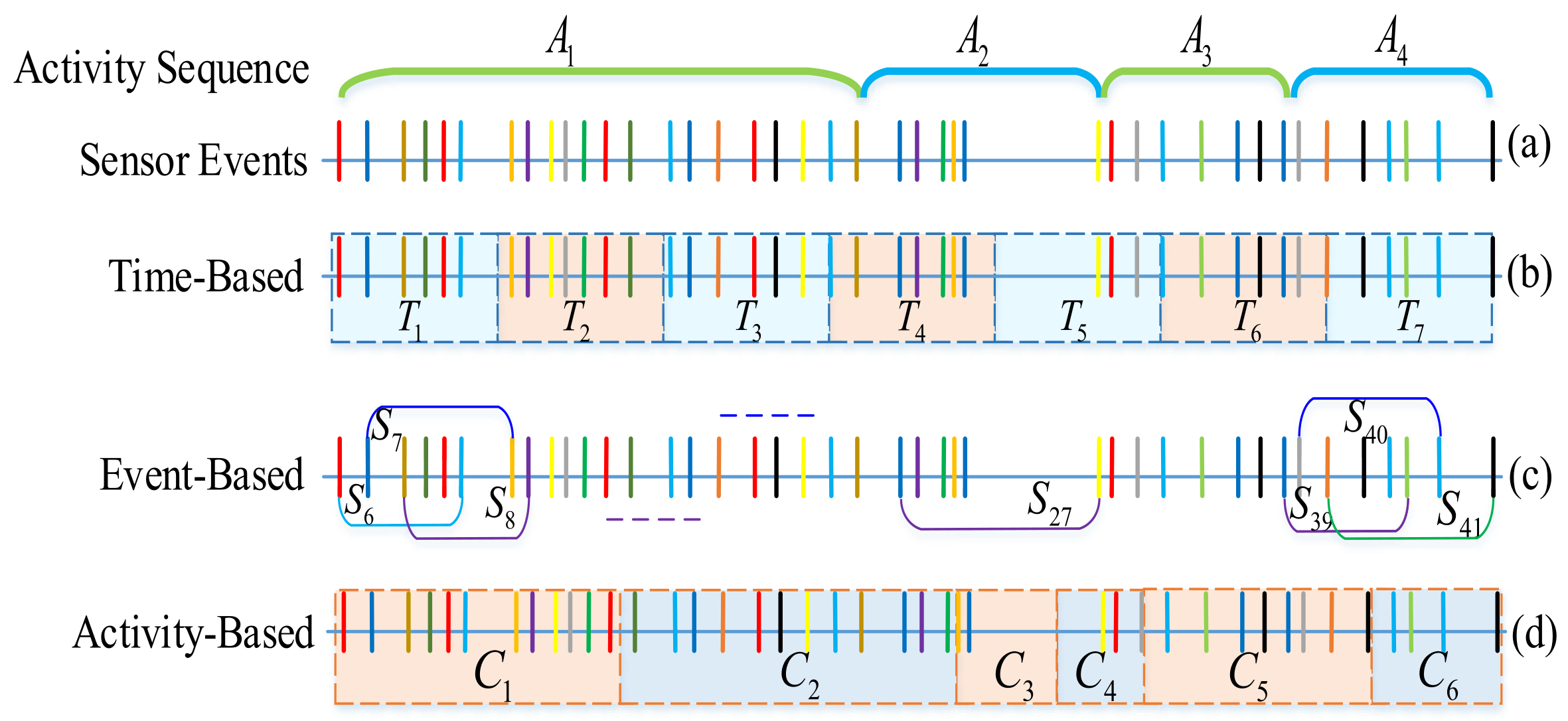
- The dynamic streaming sensor data segmentation approach incorporating sensor correlation and time correlation can reduce the probability of sensor events with large time intervals or from very different functional areas in the same sliding window, so as to weaken their influence on the context information defining the last sensor event.
- By explicitly representing the activity features extracted based on the emergent computing paradigm in the form of the directed-weighted network, the spatio-temporal characteristics can be embodied without the need of sophisticated domain knowledge, the context information defining the last event in the window can be reflected, and the ambiguity between ADLs can be relieved.
2. Related Works
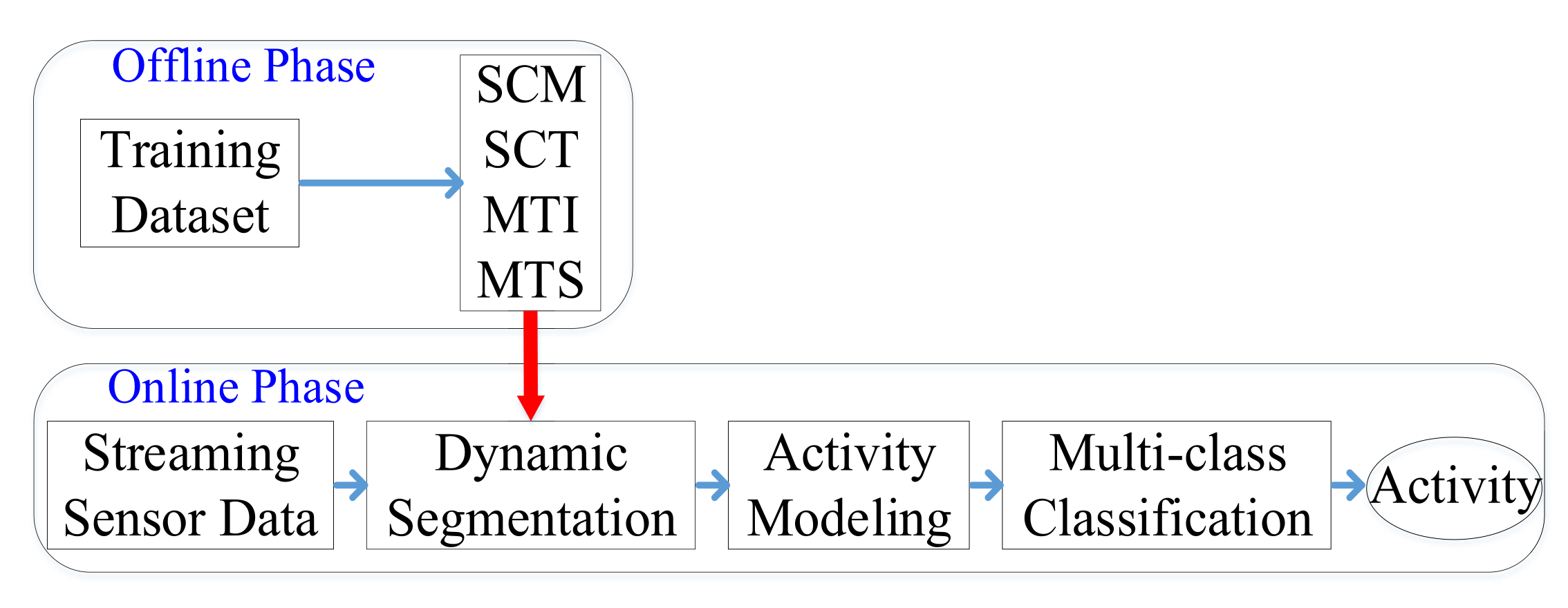
3. Online Activity Recognition Framework
3.1. Dynamic Streaming Sensor Data Segmentation
3.1.1. Sensor Correlation
3.1.2. Time Correlation
| Algorithm 1 Dynamic sensor data segmentation method. |
Input: Streaming sensor data: Initialization window for the sensor event: , Output: A sensor event segmentation for : Method: Sensor correlation check (SCC): Time correlation check (TCC): , for From To do if && && then else Break end if end for |
3.2. Activity Modeling
3.3. Fine-Grained Classification
4. Experiments
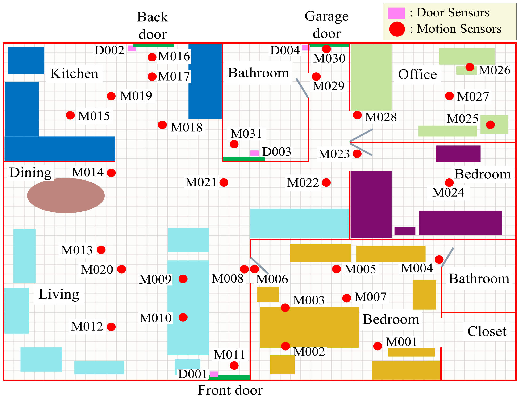
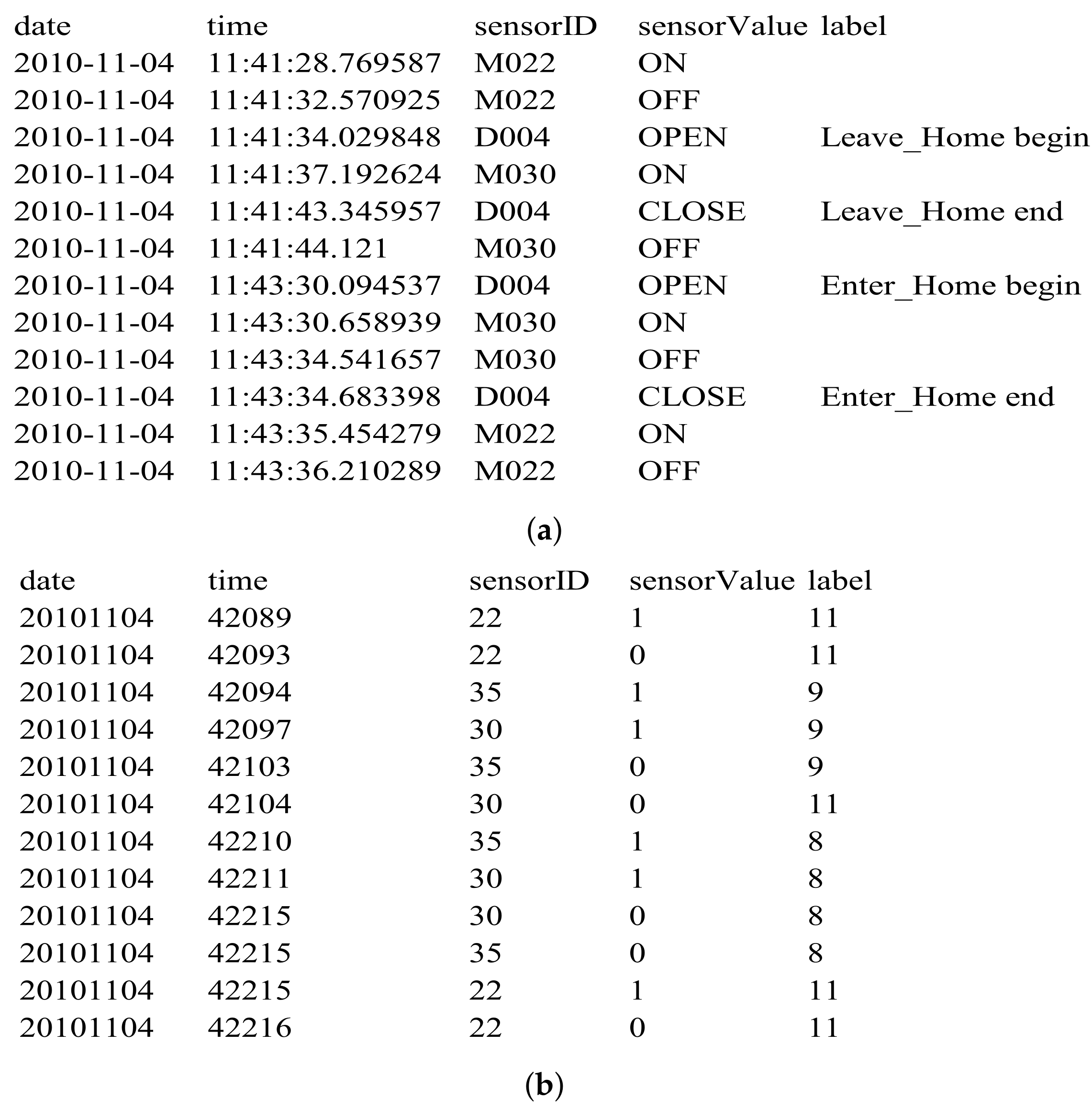
4.1. Dataset
4.2. Evaluation Measures
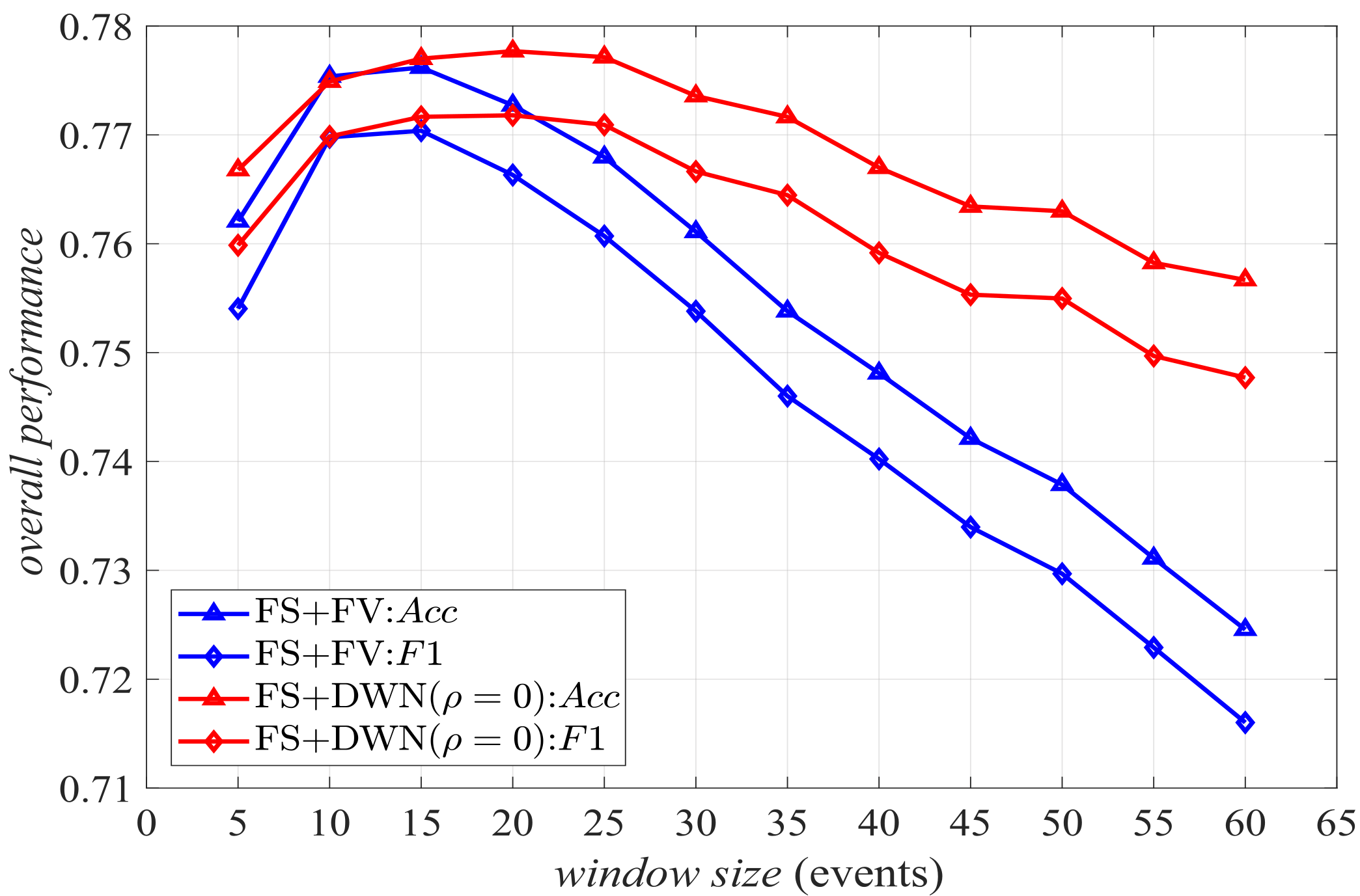
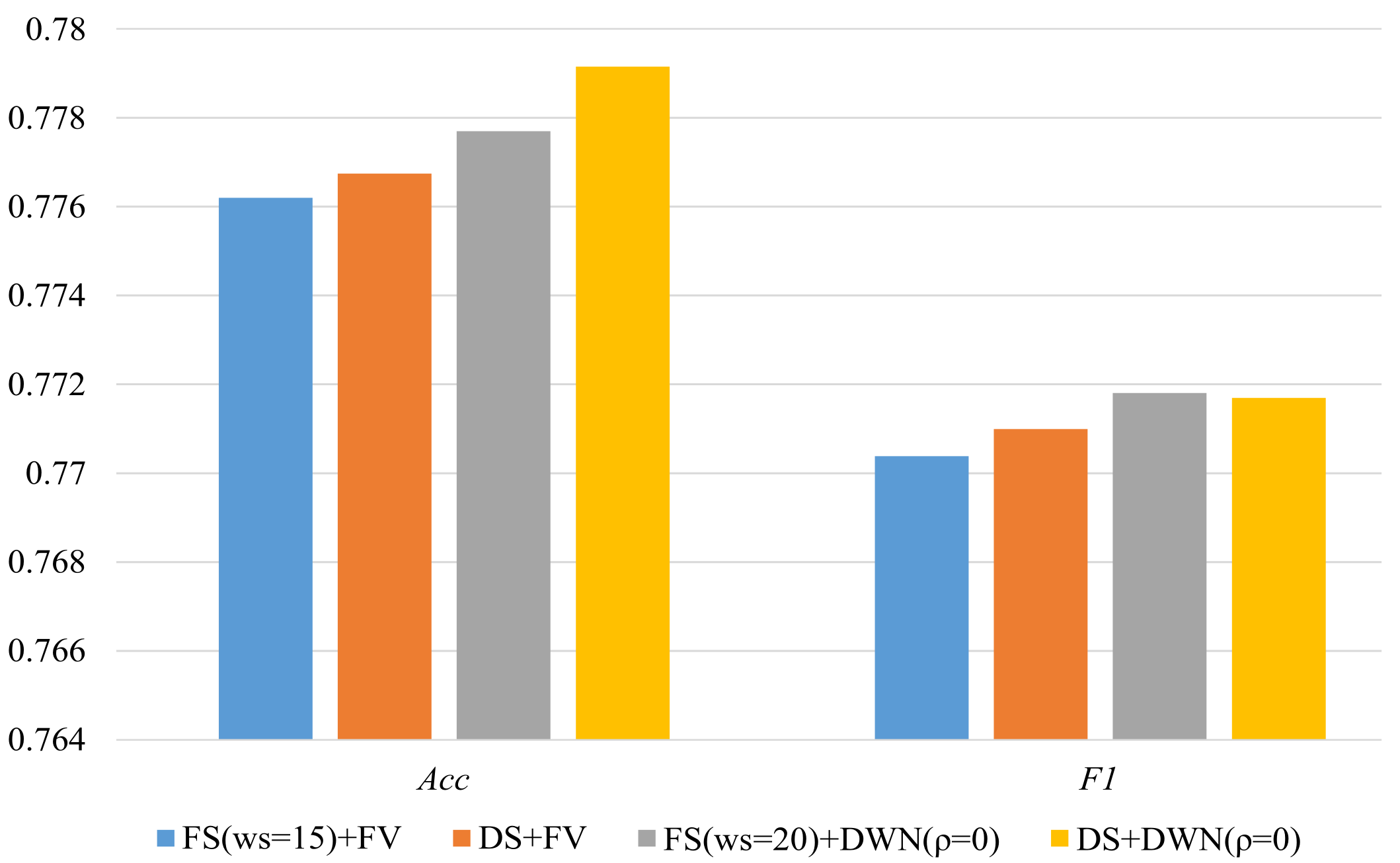
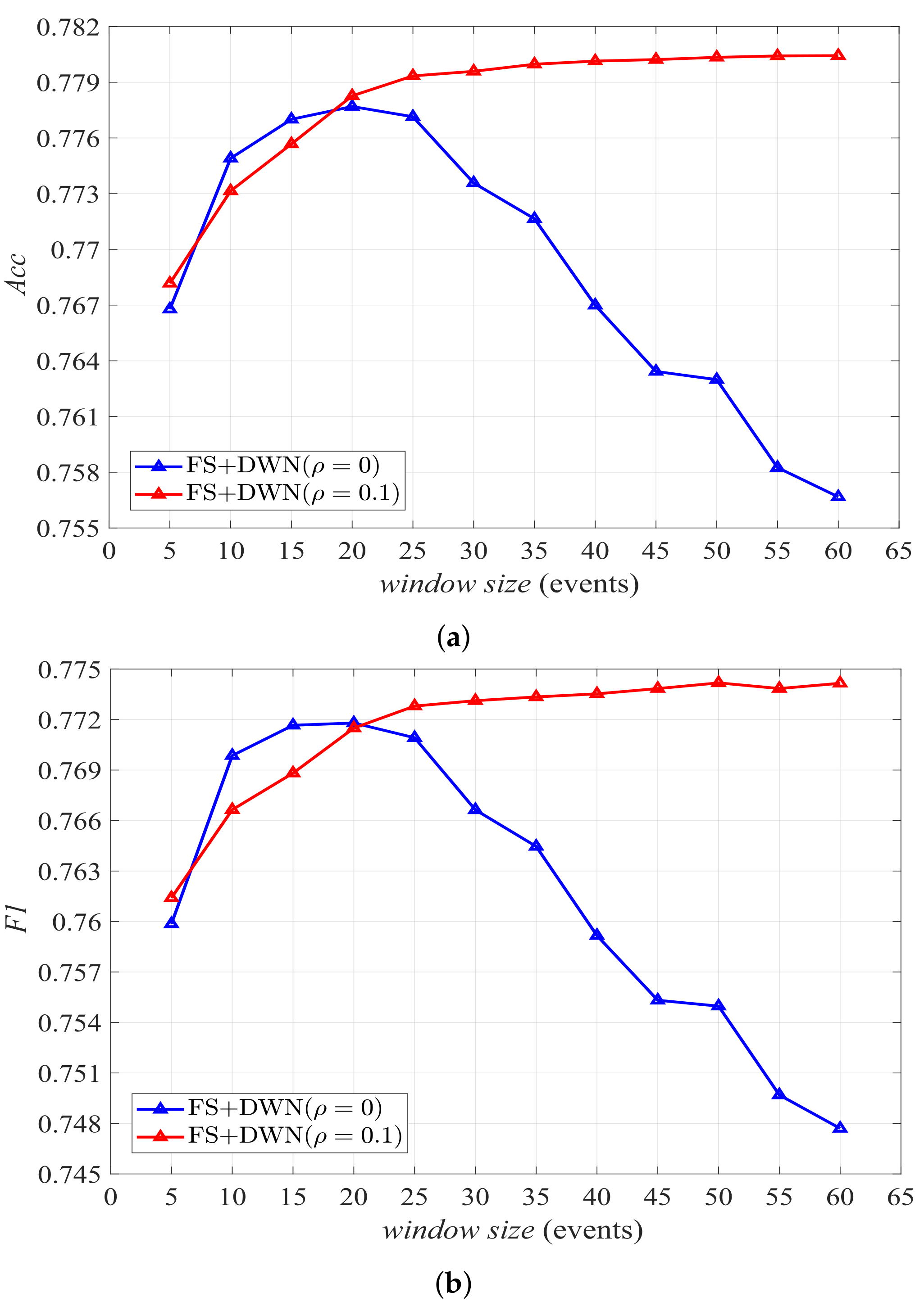
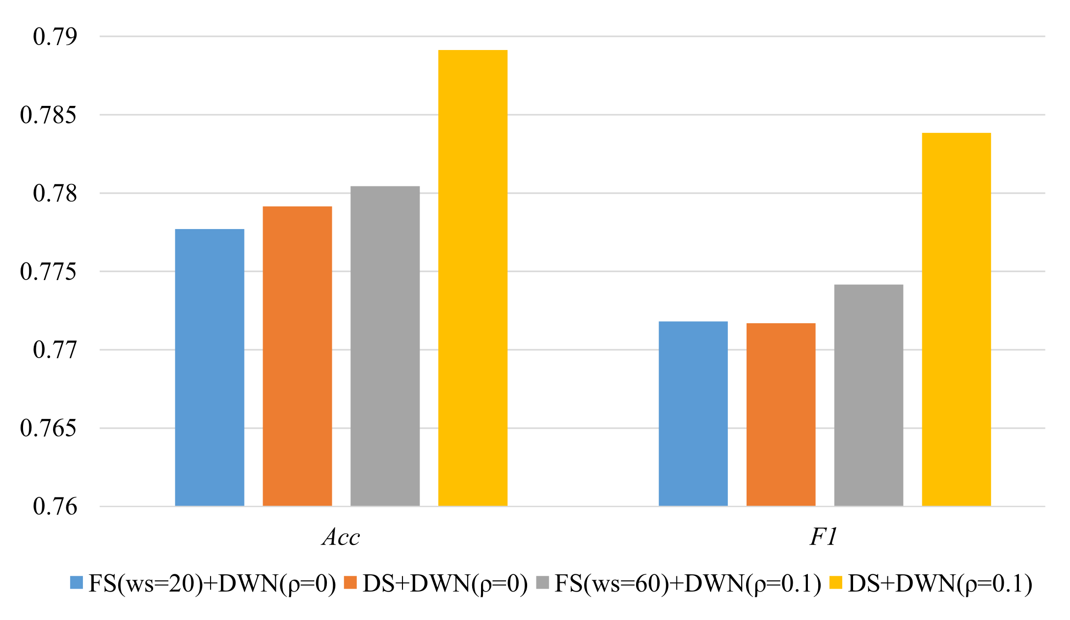
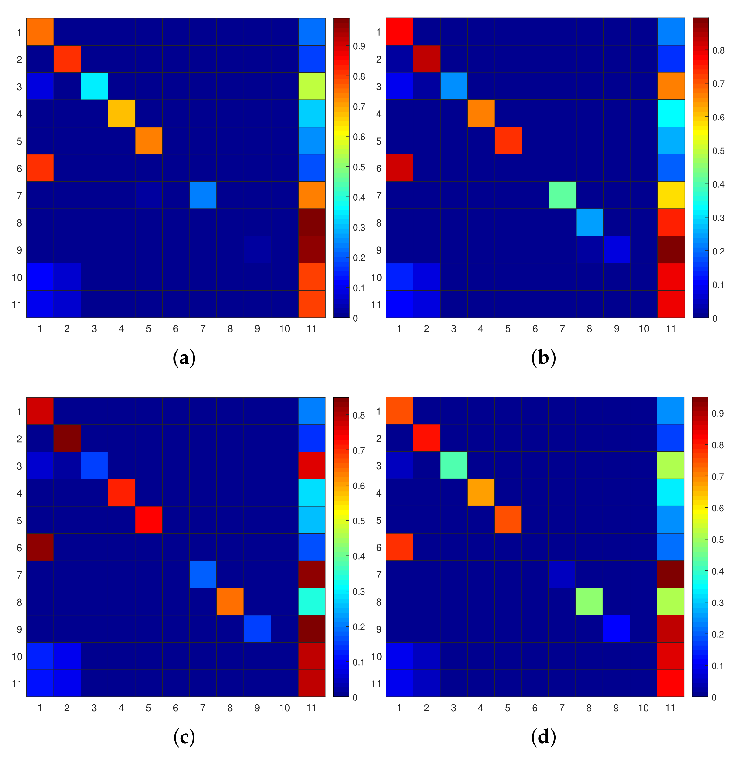
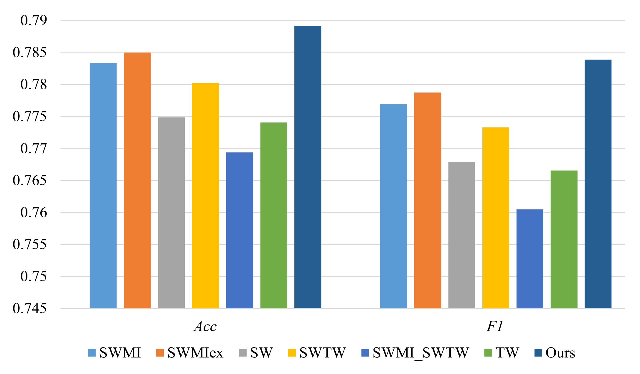
4.3. Experimental Results
5. Conclusions
Author Contributions
Funding
Institutional Review Board Statement
Informed Consent Statement
Data Availability Statement
Conflicts of Interest
References
- United Nations. World Population Prospects 2019: Highlights. Population Division of the United Nations Department of Economic and Social Affairs; United Nations: New York, NY, USA, 2019. [Google Scholar]
- Mirzaie, M.; Darabi, S. Population aging in Iran and rising health care costs. Iran. J. Ageing 2017, 12, 156–169. [Google Scholar] [CrossRef]
- Gochoo, M.; Tan, T.H.; Velusamy, V.; Liu, S.H.; Bayanduuren, D.; Huang, S.C. Device-free non-privacy invasive classification of elderly travel patterns in a smart house using PIR sensors and DCNN. IEEE Sens. J. 2018, 18, 390–400. [Google Scholar] [CrossRef]
- Pollack, M.E.; Brown, L.; Colbry, D.; McCarthy, C.E.; Orosz, C.; Peintner, B.; Ramakrishnan, S.; Tsamardinos, I. Autominder: An intelligent cognitive orthotic system for people with memory impairment. Robot. Auton. Syst. 2003, 44, 273–282. [Google Scholar] [CrossRef]
- Das, B.; Chen, C.; Seelye, A.M.; Cook, D.J. An automated prompting system for smart environments. In Proceedings of the 9th International Conference on Smart Homes and Health Telematics (ICOST 2011), Montreal, QC, Canada, 20–22 June 2011; pp. 9–16. [Google Scholar]
- Yan, S.; Liao, Y.; Feng, X.; Liu, Y. Real time activity recognition on streaming sensor data for smart environments. In Proceedings of the 4th IEEE International Conference on Progress in Informatics and Computing (IEEE PIC), Shanghai, China, 23–25 December 2016; pp. 51–55. [Google Scholar]
- Fu, T.C. A review on time series data mining. Eng. Appl. Artif. Intell. 2011, 24, 164–181. [Google Scholar] [CrossRef]
- Mortazavi, B.; Nemati, E.; VanderWall, K.; Flores-Rodriguez, H.G.; Cai, J.Y.J.; Lucier, J.; Naeim, A.; Sarrafzadeh, M. Can smartwatches replace smartphones for posture tracking? Sensors 2015, 15, 26783–26800. [Google Scholar] [CrossRef] [Green Version]
- Laudanski, A.; Brouwer, B.; Li, Q. Activity classification in persons with stroke based on frequency features. Med. Eng. Phys. 2015, 37, 180–186. [Google Scholar] [CrossRef] [PubMed]
- Suto, J.; Oniga, S.; Sitar, P.P. Feature analysis to human activity recognition. Int. J. Comput. Commun. 2016, 12, 116–130. [Google Scholar] [CrossRef]
- Barsocchi, P.; Cimino, M.G.; Ferro, E.; Lazzeri, A.; Palumbo, F.; Vaglini, G. Monitoring elderly behavior via indoor position-based stigmergy. Pervasive Mob. Comput. 2015, 23, 26–42. [Google Scholar] [CrossRef]
- Xu, Z.; Wang, G.; Guo, X. Sensor-based activity recognition of solitary elderly via stigmergy and two-layer framework. Eng. Appl. Artif. Intell. 2020, 95, 103859. [Google Scholar] [CrossRef]
- Cook, D.J.; Crandall, A.S.; Thomas, B.L.; Krishnan, N.C. CASAS: A smart home in a box. Computer 2012, 46, 62–69. [Google Scholar] [CrossRef] [PubMed] [Green Version]
- Beddiar, D.R.; Nini, B.; Sabokrou, M.; Hadid, A. Vision-based human activity recognition: A survey. Multimed. Tools Appl. 2020, 79, 30509–30555. [Google Scholar] [CrossRef]
- Nweke, H.F.; Teh, Y.W.; Al-Garadi, M.A.; Alo, U.R. Deep learning algorithms for human activity recognition using mobile and wearable sensor networks: State of the art and research challenges. Expert Syst. Appl. 2018, 105, 233–261. [Google Scholar] [CrossRef]
- Fu, Z.; He, X.; Wang, E.; Huo, J.; Huang, J.; Wu, D. Personalized human activity recognition based on integrated wearable sensor and transfer learning. Sensors 2021, 21, 885. [Google Scholar] [CrossRef] [PubMed]
- Tan, Z.; Xu, L.; Zhong, W.; Guo, X.; Wang, G. Online activity recognition and daily habit modeling for solitary elderly through indoor position-based stigmergy. Eng. Appl. Artif. Intell. 2018, 76, 214–225. [Google Scholar] [CrossRef]
- Gochoo, M.; Tan, T.H.; Liu, S.H.; Jean, F.R.; Alnajjar, F.S.; Huang, S.C. Unobtrusive activity recognition of elderly people living alone using anonymous binary sensors and DCNN. IEEE J. Biomed. Health 2019, 23, 693–702. [Google Scholar] [CrossRef]
- Al Machot, F.; Mosa, A.H.; Ali, M.; Kyamakya, K. Activity recognition in sensor data streams for active and assisted living environments. IEEE Trans. Circuits Syst. Video Technol. 2017, 28, 2933–2945. [Google Scholar] [CrossRef]
- Tan, T.H.; Badarch, L.; Zeng, W.X.; Gochoo, M.; Alnajjar, F.S.; Hsieh, J.W. Binary sensors-based privacy-preserved activity recognition of elderly living alone using an RNN. Sensors 2021, 21, 5371. [Google Scholar] [CrossRef] [PubMed]
- Patterson, D.J.; Fox, D.; Kautz, H.; Philipose, M. Fine-grained activity recognition by aggregating abstract object usage. In Proceedings of the 9th International Symposium on Wearable Computers, Osaka, Japan, 18–21 October 2005; pp. 44–51. [Google Scholar]
- Asghari, P.; Soleimani, E.; Nazerfard, E. Online human activity recognition employing hierarchical hidden Markov models. J. Ambient Intell. Humaniz. Comput. 2020, 11, 1141–1152. [Google Scholar] [CrossRef] [Green Version]
- Fan, C.; Gao, F. Enhanced human activity recognition using wearable sensors via a hybrid feature selection method. Sensors 2021, 21, 6434. [Google Scholar] [CrossRef] [PubMed]
- Tapia, E.M.; Intille, S.S.; Larson, K. Activity recognition in the home using simple and ubiquitous sensors. In Proceedings of the 2nd International Conference on Pervasive Computing, Linz, Austria, 18–23 April 2004; pp. 158–175. [Google Scholar]
- Lee, S.W.; Mase, K. Activity and location recognition using wearable sensors. IEEE Pervasive Comput. 2002, 1, 24–32. [Google Scholar]
- Huynh, T.; Blanke, U.; Schiele, B. Scalable recognition of daily activities with wearable sensors. In Proceedings of the 3rd International Symposium on Location- and Contest-Awareness (LoCA 2007), Oberpfaffenhofen, Germany, 20–21 September 2007; pp. 50–67. [Google Scholar]
- Liao, L.; Fox, D.; Kautz, H. Extracting places and activities from GPS traces using hierarchical conditional random fields. In Proceedings of the 12th International Symposium on Robotics Research (ISRR), San Francisco, CA, USA, 12–15 October 2005; pp. 119–134. [Google Scholar]
- Van Kasteren, T.; Englebienne, G.; Kröse, B.J. Activity recognition using semi-Markov models on real world smart home datasets. J. Ambient Intell. Smart Environ. 2010, 2, 311–325. [Google Scholar] [CrossRef] [Green Version]
- Huynh, T.; Schiele, B. Unsupervised discovery of structure in activity data using multiple eigenspaces. In Proceedings of the 2nd International Workshop on Location- and Context-Awareness (LoCA 2006), Dublin, Ireland, 10–11 May 2006; pp. 151–167. [Google Scholar]
- Abdellaoui, M.; Douik, A. Human action recognition in video sequences using deep belief networks. Trait. Signal 2020, 37, 37–44. [Google Scholar] [CrossRef] [Green Version]
- Mohmed, G.; Lotfi, A.; Pourabdollah, A. Enhanced fuzzy finite state machine for human activity modelling and recognition. J. Ambient Intell. Humaniz. Comput. 2020, 11, 6077–6091. [Google Scholar] [CrossRef]
- Mutegeki, R.; Han, D.S. A CNN-LSTM approach to human activity recognition. In Proceedings of the 2020 International Conference on Artificial Intelligence in Information and Communication (ICAIIC), Fukuoka, Japan, 19–21 February 2020; pp. 362–366. [Google Scholar]
- Krishnan, N.C.; Cook, D.J. Activity recognition on streaming sensor data. Pervasive Mob. Comput. 2014, 10, 138–154. [Google Scholar] [CrossRef] [PubMed] [Green Version]
- Chen, L.; Nugent, C.D.; Wang, H. A knowledge-driven approach to activity recognition in smart homes. IEEE Trans. Knowl. Data Eng. 2011, 24, 961–974. [Google Scholar] [CrossRef]
- Okeyo, G.; Chen, L.; Wang, H.; Sterritt, R. Dynamic sensor data segmentation for real-time knowledge-driven activity recognition. Pervasive Mob. Comput. 2014, 10, 155–172. [Google Scholar] [CrossRef]
- Sfar, H.; Bouzeghoub, A. DataSeg: Dynamic streaming sensor data segmentation for activity recognition. In Proceedings of the 34th ACM/SIGAPP Annual International Symposium on Applied Computing (SAC), Limassol, Cyprus, 8–12 April 2019; University Cyprus: Limassol, Cyprus, 2019; pp. 557–563. [Google Scholar]
- Yala, N.; Fergani, B.; Fleury, A. Feature extraction for human activity recognition on streaming data. In Proceedings of the International Symposium on Innovations in Intelligent SysTems and Applications (INISTA 2015), Madrid, Spain, 2–4 September 2015; pp. 1–6. [Google Scholar]
- Yala, N.; Fergani, B.; Fleury, A. Towards improving feature extraction and classification for activity recognition on streaming data. J. Ambient Intell. Humaniz. Comput. 2017, 8, 177–189. [Google Scholar] [CrossRef] [Green Version]


| Activity Name | Number of Events | Proportion (%) |
|---|---|---|
| 1-Meal_Preparation | 288,407 | 18.06370999 |
| 2-Relax | 347,911 | 21.79060635 |
| 3-Eating | 16,352 | 1.02416996 |
| 4-Work | 16,321 | 1.022228346 |
| 5-Sleeping | 32,535 | 2.037754993 |
| 6-Wash_Dishes | 10,417 | 0.652444868 |
| 7-Bed_to_Toilet | 1310 | 0.082048841 |
| 8-Enter_Home | 2003 | 0.125453304 |
| 9-Leave_Home | 1914 | 0.119878994 |
| 10-Housekeeping | 10,579 | 0.662591365 |
| 11-Other Activity | 868,861 | 54.419113 |
| Confusion Matrix | Predicted Result | ||
|---|---|---|---|
| Positive | Negtive | ||
| True Result | True | True Positive () | False Negtive () |
| False | False Positive () | True Negative () | |
Publisher’s Note: MDPI stays neutral with regard to jurisdictional claims in published maps and institutional affiliations. |
© 2022 by the authors. Licensee MDPI, Basel, Switzerland. This article is an open access article distributed under the terms and conditions of the Creative Commons Attribution (CC BY) license (https://creativecommons.org/licenses/by/4.0/).
Share and Cite
Xu, Z.; Wang, G.; Guo, X. Online Activity Recognition Combining Dynamic Segmentation and Emergent Modeling. Sensors 2022, 22, 2250. https://doi.org/10.3390/s22062250
Xu Z, Wang G, Guo X. Online Activity Recognition Combining Dynamic Segmentation and Emergent Modeling. Sensors. 2022; 22(6):2250. https://doi.org/10.3390/s22062250
Chicago/Turabian StyleXu, Zimin, Guoli Wang, and Xuemei Guo. 2022. "Online Activity Recognition Combining Dynamic Segmentation and Emergent Modeling" Sensors 22, no. 6: 2250. https://doi.org/10.3390/s22062250