1. Introduction
Digital images are increasingly used in several vision application domains of everyday life, such as medical imaging [
1,
2], object recognition in images [
3], autonomous vehicles [
4], Internet of Things (
) [
5], computer-aided diagnosis [
6], and
mapping [
7]. In all these applications, the produced images are subject to a wide variety of distortions during acquisition, compression, transmission, storage, and displaying. These distortions lead to a degradation of visual quality [
8]. The increasing demand for images in a wide variety of applications involves perpetual improvement of the quality of the used images. As each domain has different thresholds in terms of visual perception needed and fault tolerance, so, equally, does the importance of visual perception quality assessment.
As human beings are the final users and interpreters of image processing, subjective methods based on the human ranking score are the best processes to evaluate image quality. The ranking consists of asking several people to watch images and rate their quality. In practice, subjective methods are generally too expensive, time-consuming, and not usable in real-time applications [
8,
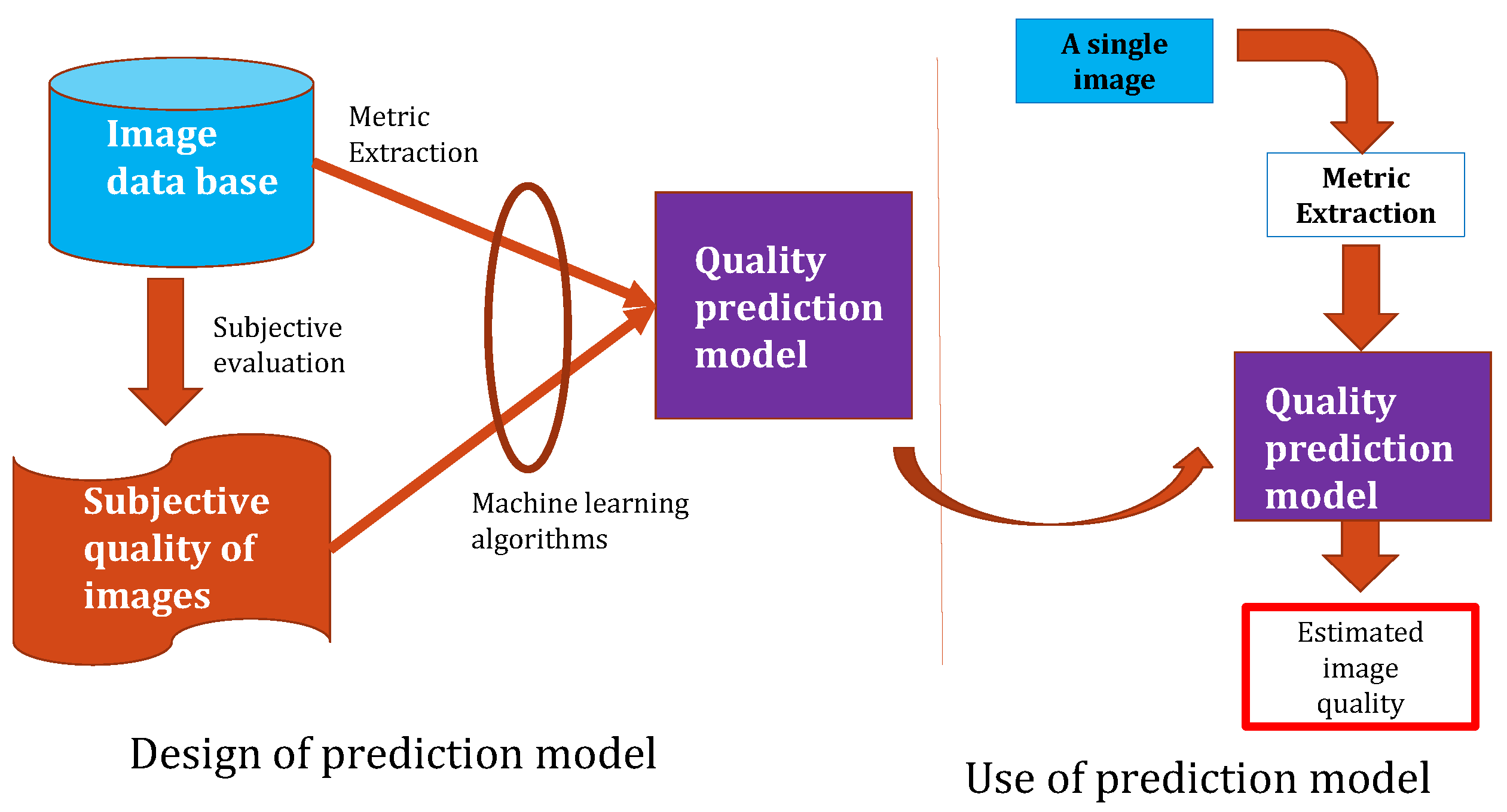
9]. Thus, many research works have focused on objective image quality assessment
methods aiming to develop quantitative measures that automatically predict image quality [
2,
8,
10]. The objective
process is illustrated in
Figure 1. This process has been introduced in the paper [
11].
In digital image processing, objective
can be used for several roles, such as dynamic monitoring and adjusting the image quality, benchmark and optimize image processing algorithms, and parameter setting of image processing [
8,
12]. Many research investigations explore the use of machine learning (
) algorithms in order to build objective
models in agreement with human visual perception. Recent methods include, artificial neural network (
), support vector machine (
), nonlinear regression (
), decision tree (
), clustering, and fuzzy logic (
) [
13]. After the propulsion of deep learning techniques in 2012 [
14], researchers were also interested in the possibility of using these techniques in the image quality assessment. Thus, in 2014, the first studies emerged on the use of convolutional neural networks in
[
15]. Many other works have followed, and we find in the literature increasingly efficient
models [
16,
17,
18].
The
evaluation methods can be classified into three categories according to whether or not they require a reference image: full-reference (
), reduced-reference (
), and no-reference (
)
approaches. Full reference image quality assessment (
-
) needs a complete reference image in order to be computed. Among the most popular
-
, we can cite the peak signal to noise ratio (
), structure similarity index metric (
) [
8,
19], and visual information fidelity (
) [
20]. In reduced reference image quality assessment (
-
), the reference image is only partially available, in the form of a set of extracted features, which help to evaluate the distorted image quality; this is the case of reduced reference entropic differencing (
) [
21]. In many real-life applications, the reference image is unfortunately not available. Therefore, for this application, the need of no-reference image quality assessment (
-
) methods or blind
(
), which automatically predict the perceived quality of distorted images, without any knowledge of reference image. Some
-
methods assume the type of distortions are previously known [
22,
23], these objective assessment techniques are called distortion specific (
)
-
. They can be used to assess the quality of images distorted by some particular distortion types. As example, the algorithm in [
23] is for
compressed images, while in [
22] it is for
compressed images, and in [
24] it is for detection of blur distortion. However, in most practical applications, information about the type of distortion is not available. Therefore, it is more relevant to design non-distortion specific (
)
-
methods that examine image without prior knowledge of specific distortions [
25]. Many existing metrics are the base units used in
methods, such as
[
26],
-
[
27],
[
28],
[
29],
[
30],
[
31], DIQA [
32], and DIQa-NR [
33].
The proposal of this paper is a non-distortion-specific
-
approach, where the extracted features are based on a combination of the natural scene statistic in the spatial domain [
28], the gradient magnitude [
29], the Laplacian of Gaussian [
29], as well as the spatial and spectral entropies [
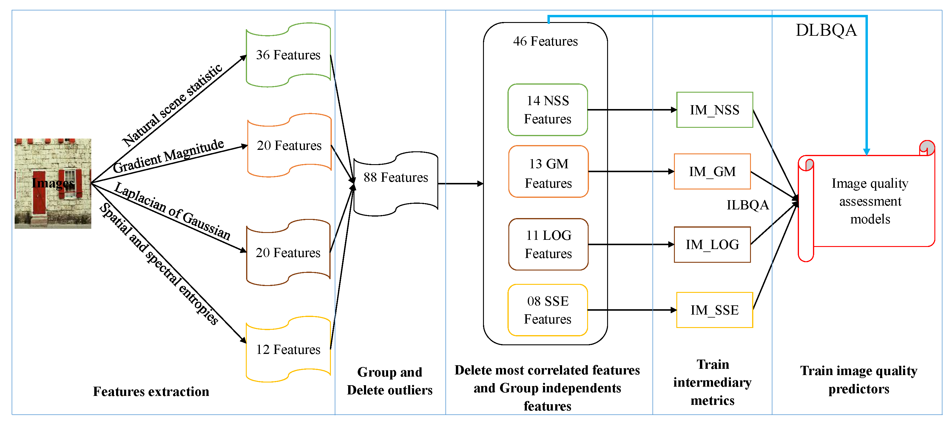
30]. These features are trained using machine learning methods to construct the models used to predict the perceived image quality. The process we propose for designing the evaluation of perceived no-reference image quality models is described in
Figure 2. The process consists of
extracting the features from images taken in the databases,
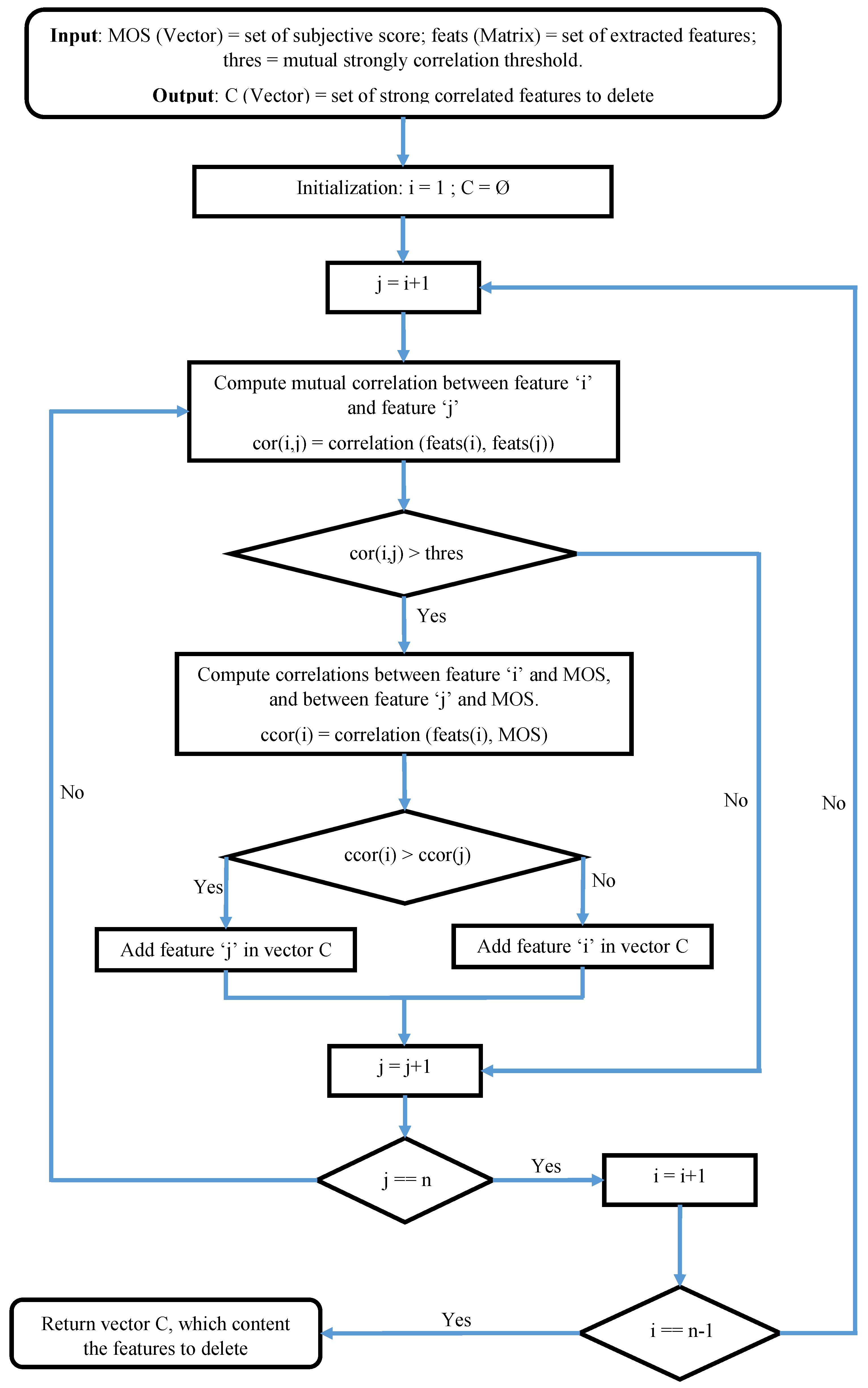
removing the superfluous features according to the correlation between the extracted features,
grouping the linearly independent features to construct some intermediate metrics, and
using the produced metrics to construct the estimator model for perceived image quality assessment.
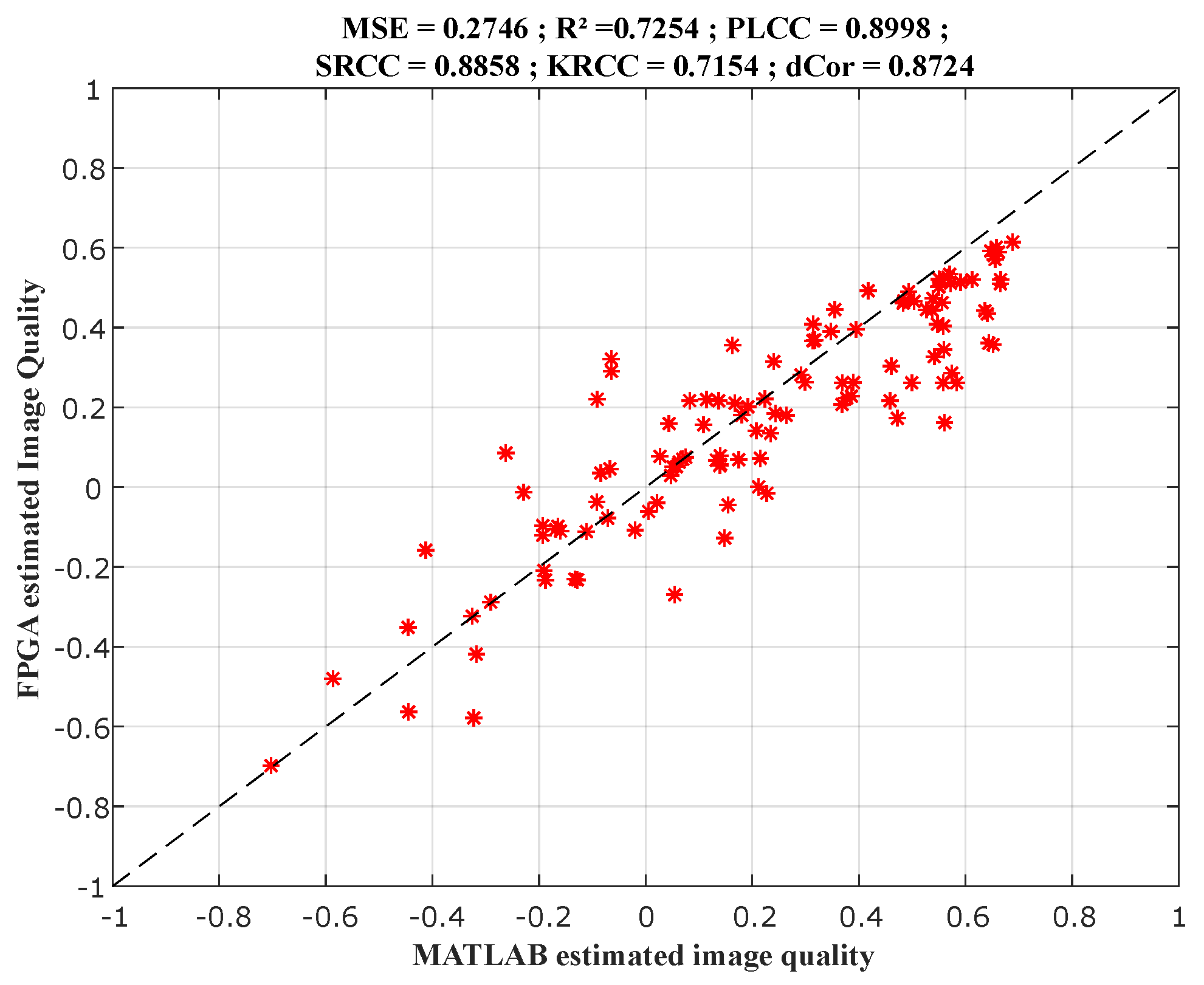
Finally, we compare the designed models with the state-of-the-art models using the features extraction, but also the process using deep learning with convolutional neural network; as shown in
Section 4.1.
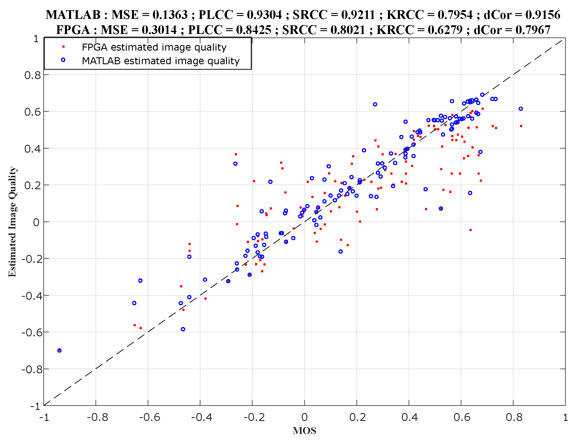
To evaluate the performances of the produced models, we measure the correlation between objective and subjective quality scores using three correlation coefficients:
- (1)
Pearson’s linear correlation coefficient (), which is used to measure the degree of the relationship between linear related variables.
- (2)
Spearman’s rank order correlation coefficient (), which is used to measure the prediction monotony and the degree of association between two variables.
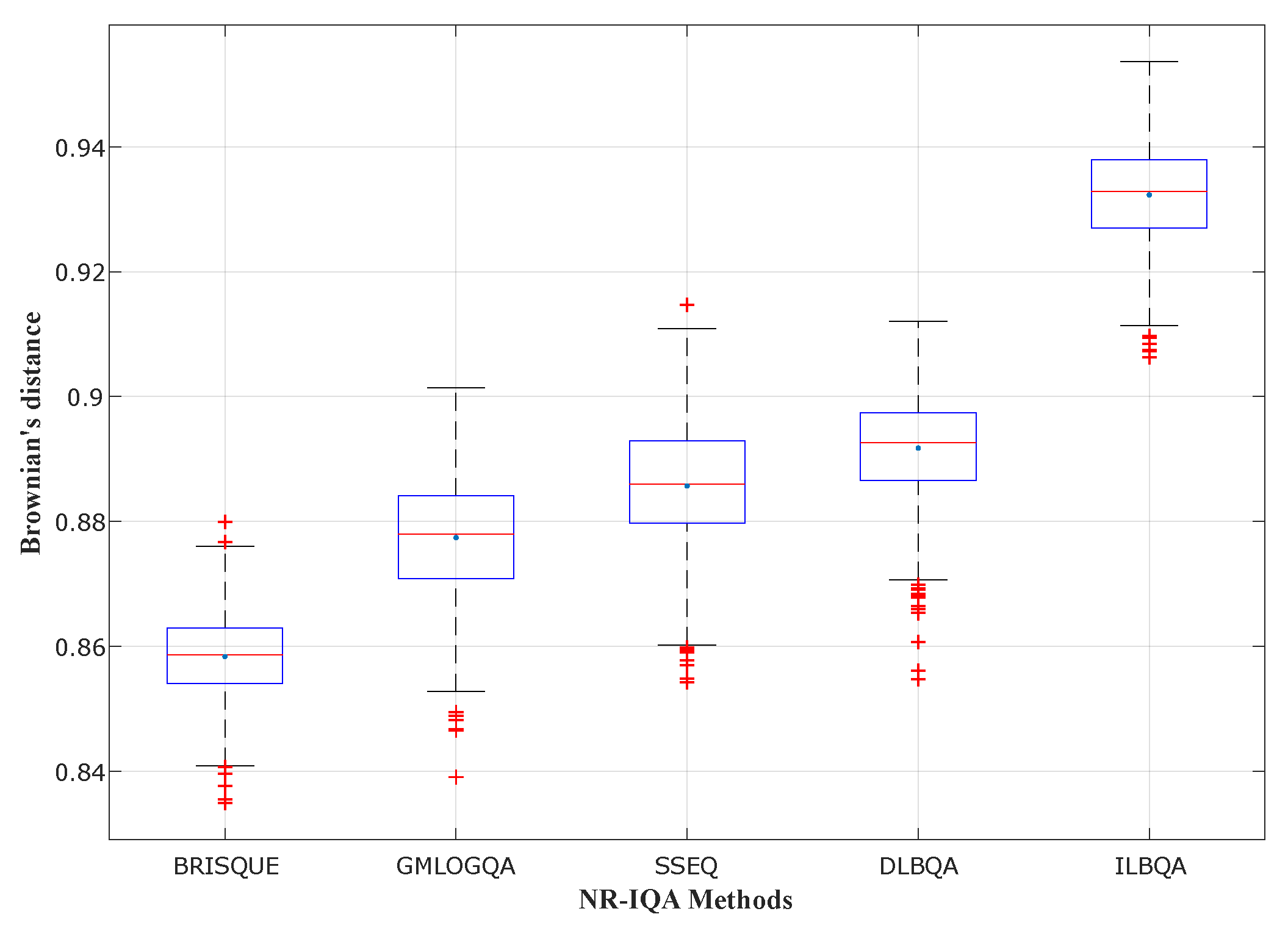
- (3)
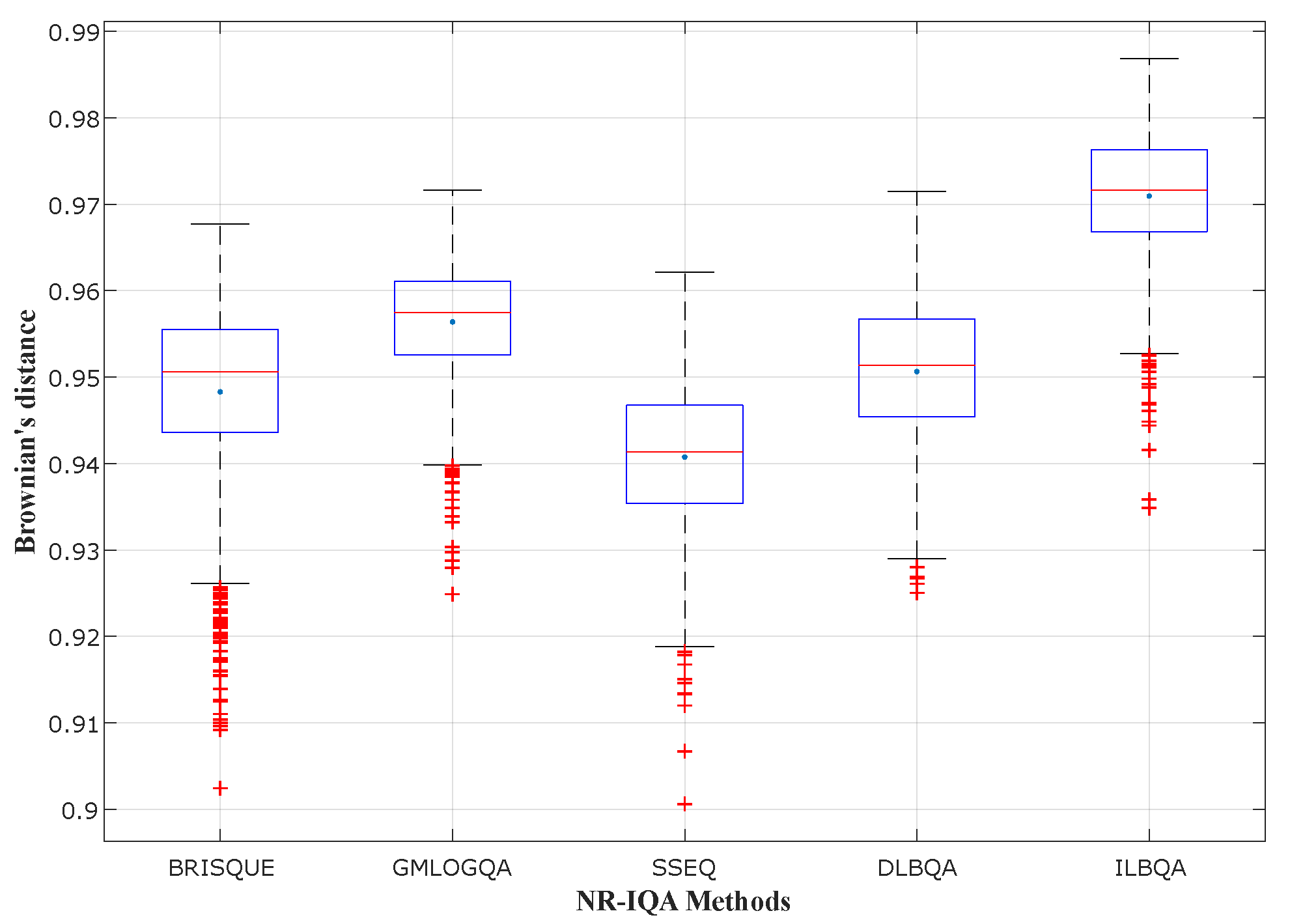
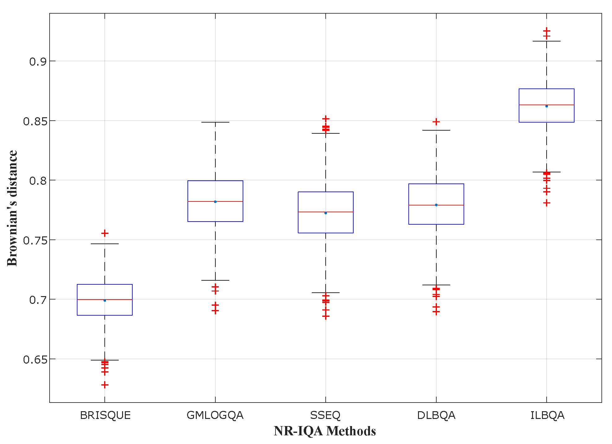
Brownian distance (), which is a measure of statistical dependence between two random variables or two random vectors of arbitrary, not necessarily equal dimension.
The paper is organized as follows.
Section 2 presents the feature extraction methods.
Section 3 explains the feature selection technique based on feature independence analysis. The construction of intermediate metrics is also presented in this section.
Section 4 explains the experimental results and their comparison.
Section 5 presents the
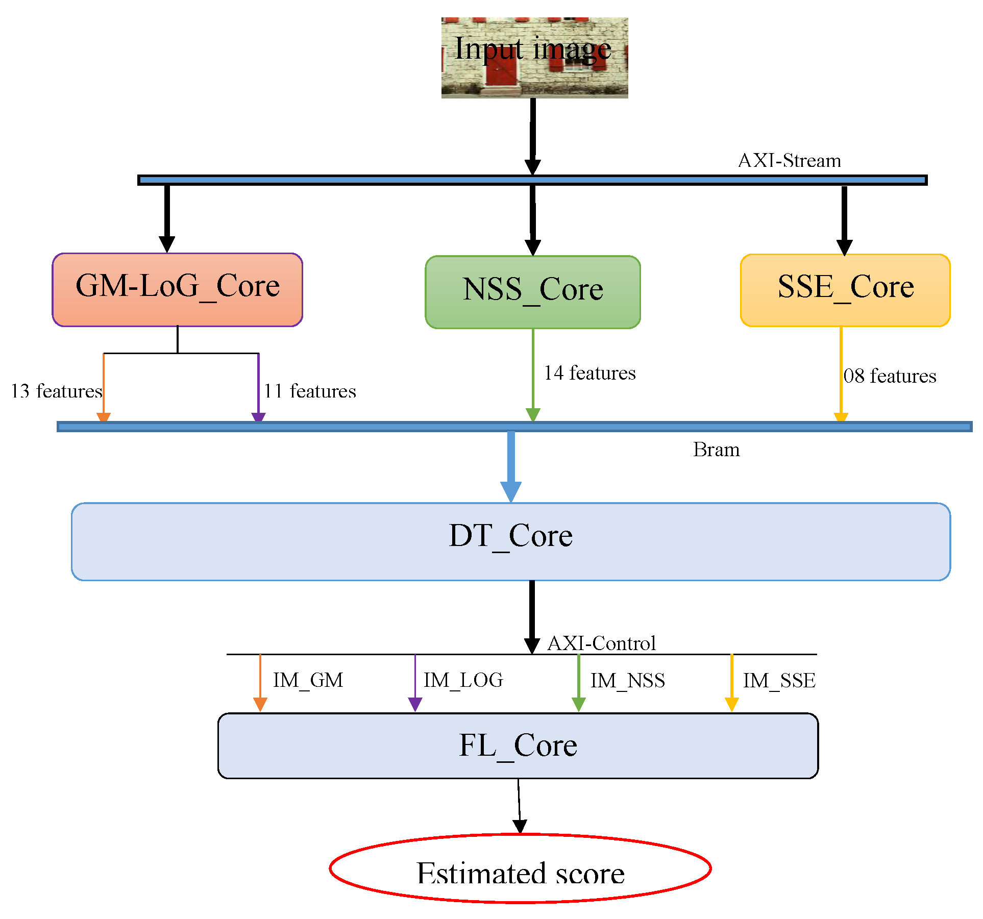
implementation architectures and results. Finally,
Section 6 draws a conclusion and perspectives for future investigations.
2. Feature Extraction
Feature extraction in this paper is based on four principal axes: natural scene statistic in the spatial domain, gradient magnitude, Laplacian of Gaussian, and finally spatial and spectral entropies.
2.1. Natural Scene Statistic in the Spatial Domain
The extraction of the features based on
in spatial domain starts by normalization of the image represented by
, to remove local mean displacements from zero log-contrast, and to normalize the local variance of the log contrast as observe in [
34]. Equation (
1) presents normalization of the initial image.
where
i and
j are the spatial indices, M and N are the image dimensions,
and
.
that denotes the local mean is represented by (
2) and
that estimates the local contract is expressed by (
3).
where
, and
.
is a 2D circularly-symmetric Gaussian weighting function sampled out to 3 standard deviations (
) and rescaled to unit volume [
28].
The model produced in (
1) is used as the mean-subtracted contrast normalized (
) coefficients. In [
28], they take the hypothesis that the
coefficients have characteristic statistical properties that are changed by the presence of distortion. Quantifying these changes helps predict the type of distortion affecting an image as well as its perceptual quality. They also found that a Generalized Gaussian Distribution (
) could be used to effectively capture a broader spectrum of a distorted image, where the
with zero mean is given by (
4).
where
is represented by (
5) and
is expressed by (
6).
The parameter controls the shape of the distribution while controls the variance.
In [
28], they also give the statistical relationships between neighboring pixels along four orientations:
and
. This is used with asymmetric density function to produce a practical alternative to adopt a general asymmetric generalized Gaussian distribution (
) model [
35]. Equation (
7) gives the AGGD with zero mode.
where
(with
) is given by (
8).
The parameter
controls the shape of the distribution, while
and
are scale parameters that control the spread on each side of the mode. The fourth asymmetric parameter is
given by (
9)
Finally, the founded parameters are composed of the symmetric parameters (
and
) and the asymmetric parameters (
, and
), where the asymmetric parameters are computed for the four orientations, as shown in
Table 1. All the founded parameters are also computed for two scales, yielding 36 features (2 scales × [2 symmetric parameters
asymmetric parameters
orientations]). More details about the estimation of these parameters are given in [
28,
36].
2.2. Gradient Magnitude and Laplacian of Gaussian
The second feature extraction method is based on the joint statistics of the Gradient Magnitude (
) and the Laplacian of Gaussian (
) contrast. These two elements
and
are usually used to get the semantic structure of an image. In [
29], they also introduce another usage of these elements as features to predict local image quality.
By taking an image
I(
i,
j), its GM is represented by (
10).
where ⊗ is the linear convolution operator, and
is the Gaussian partial derivative filter applied along the direction
, represented by (
11).
Moreover, the LoG of this image is represented by (
12).
where
To produce the used features, the first step is to normalize the
and
features map as in (
14).
where
is a small positive constant, used to avoid instabilities when
is small, and
is given by (
15).
where
; and
is given by (
16).
Then (
17) and (
18) give the final statistic features.
where
and
, and
is the empirical probability function of G and L [
37,
38]; it can be given by (
19).
In [
29], the authors also found that the best results are obtained by setting
; thus, 40 statistical features have been produced as shown in
Table 2, 10 dimensions for each statistical features vector
and
.
2.3. Spatial and Spectral Entropies
Spatial entropy is a function of the probability distribution of the local pixel values, while spectral entropy is a function of the probability distribution of the local discrete cosine transform (
) coefficient values. The process of extracting the spatial and spectral entropies (SSE) features from images in [
30] consists of three steps:
The first step is to decompose the image into 3 scales, using bi-cubic interpolation: low, middle, and high.
The second step is to partition each scale of the image into
blocks and compute the spatial and spectral entropies within each block. The spatial entropy is given by (
20).
and spectral entropy is given by (
21).
where
is the probability of x, and
is the spectral probability gives by (
22).
where
.
In the third step, evaluate the means and skew of blocks entropy within each scales.
At the end of the three steps, 12 features are extracted from the images as seen in
Table 3. These features represent the mean and skew for spectral and spatial entropies, on 3 scales (
features).
2.4. Convolutional Neural Network for NR-IQA
In this paper, we explore the possibility of use the deep learning with convolutional neural network to build the model used to evaluate the quality of the image. In this process, the extraction of features are done by the convolution matrix, constructed using the training process with deep learning.
In CNNs, three main characteristics of convolutional layers can distinguish them from fully connected linear layers in the vision field. In the convolutional layer,
each neuron receives an image as inputs and produces an image as its output (instead of a scalar);
each synapse learns a small array of weights, which is the size of the convolutional window; and
each pixel in the output image is created by the sum of the convolutions between all synapse weights and the corresponding images.
The convolutional layer takes as input and image of dimension
with
channels, and the output value of the pixel
(the pixel of the row
r and the column
c, of the neuron
n in the layer
l) is computed by (
23).
where
are the convolution kernel dimensions of the layer
l,
is the weight of the row
i and the column
j in the convolution matrix of the synapse
s, connected to the input of the neuron
n, in the layer
l. In reality, a convolution is simply an element-wise multiplication of two matrices followed by a sum. Therefore, the 2D convolution take two matrices (which both have the same dimensions), multiply them, element-by-element, and sum the elements together. To close the convolution process in a convolutional layer, the results are then passed through an activation function.
In convolution process, a limitation of the output of the feature map is that they record the precise position of features in the input in the convolutional layers. This means that small movements in the position of the feature in the input image will result in a different feature map. This can happen with cropping, rotating, shifting, and other minor changes to the input image [
15]. In CNNs, the common approach to solving this problem is the down-sampling using the pooling layers [
39]. The down-sampling is a reduction in the resolution of an input signal while preserving important structural elements, without the fine details that are not very useful for the task. The pooling layers are used to reduce the dimensions of the feature maps. Thus, it reduces the number of parameters to learn and the amount of computation performed in the network. The pooling layer summarizes the features present in a region of the feature map generated by a convolution layer. Therefore, further operations are performed on summarized features instead of precisely positioned features generated by the convolution layer. This makes the model more robust to variations in the position of the features in the input image.
In CNNs, the most used pooling function is Max Pooling, which calculates the maximum value for each patch on the feature map. But other pooling function exist, like Average Pooling, which calculates the average value for each patch on the feature map.
Our final CNN model, called - has 10 layers: four convolutional layers with 128, 256, 128, and 64 channels, respectively; four max pooling layers; and two fully connected layers with 1024 and 512 neurons, respectively. Finally, a output layer with one neuron is computed to give the final score of the image.


