Robust Confidence Intervals for PM2.5 Concentration Measurements in the Ecuadorian Park La Carolina


Abstract
:1. Introduction
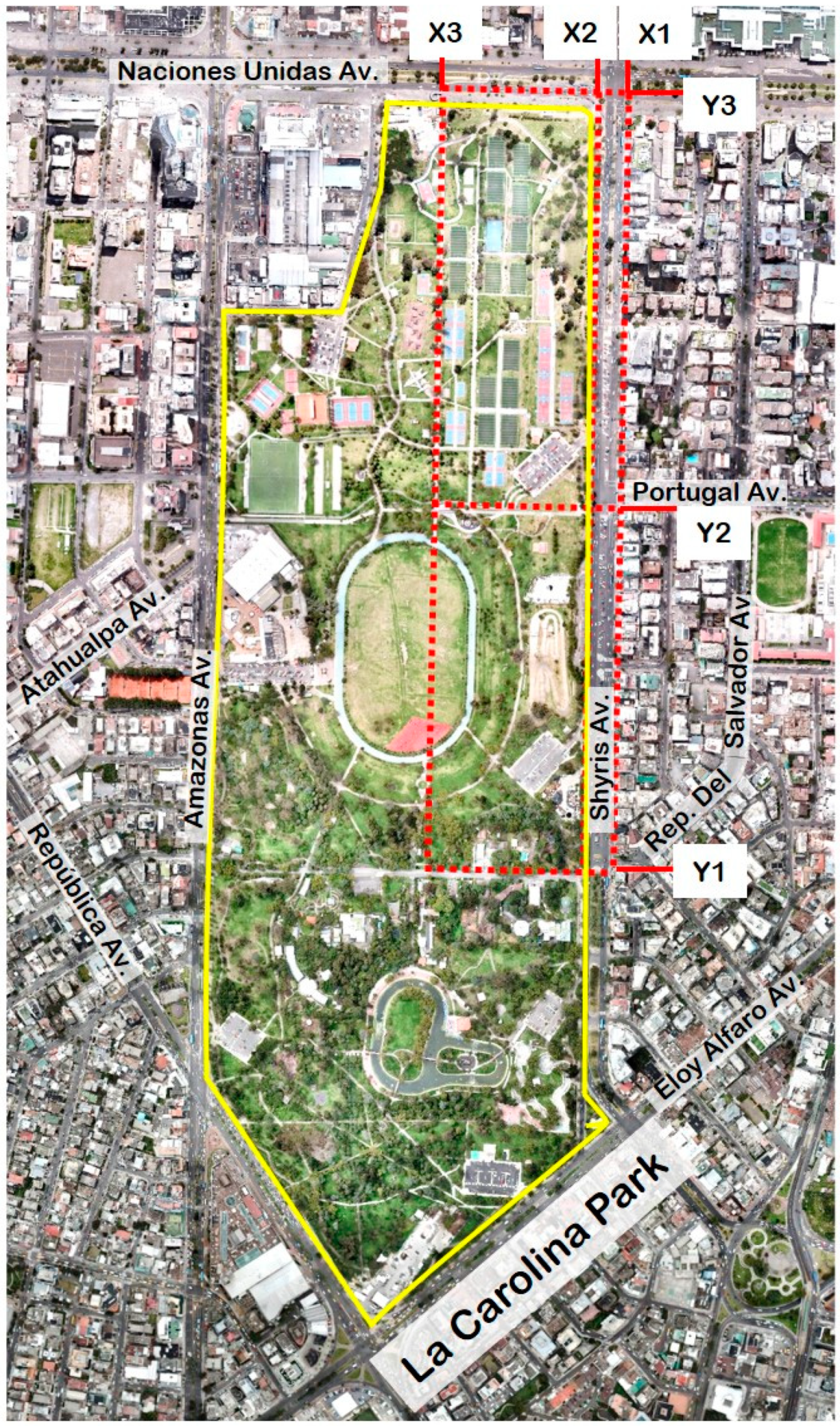
2. Study Area and Considered Data
- is a route that represents the sidewalk on Avenida de los Shyris (shown as Shyris Av. in Figure 1) that is in front of La Carolina Park.
- is a route that represents the sidewalk that is situated between La Carolina Park and Avenida de los Shyris.
- is a route through the center of the park.
- is a route through Avenida República del Salvador (shown as Rep. Del Salvador Av. in Figure 1) that people follow to go to the center of the park.
- is a route through Avenida Portugal (shown as Portugal Av. in Figure 1) that people use to go to the center of the park.
- is a route that represents the sidewalk that is situated between La Carolina Park and Avenida Naciones Unidas (shown as Naciones Unidas Av. in Figure 1).
3. Robust Confidence Intervals: Results
3.1. Method
- 1.
- Mean and standard deviation, [13].
- 2.
- Median and median absolute deviation, [13].
- 3.
- Median and semi interquartile range, [13].
- 4.
- 5.
- Andrew’s wave, [26]:IfThen
- 6.
- Biweight, [13]:
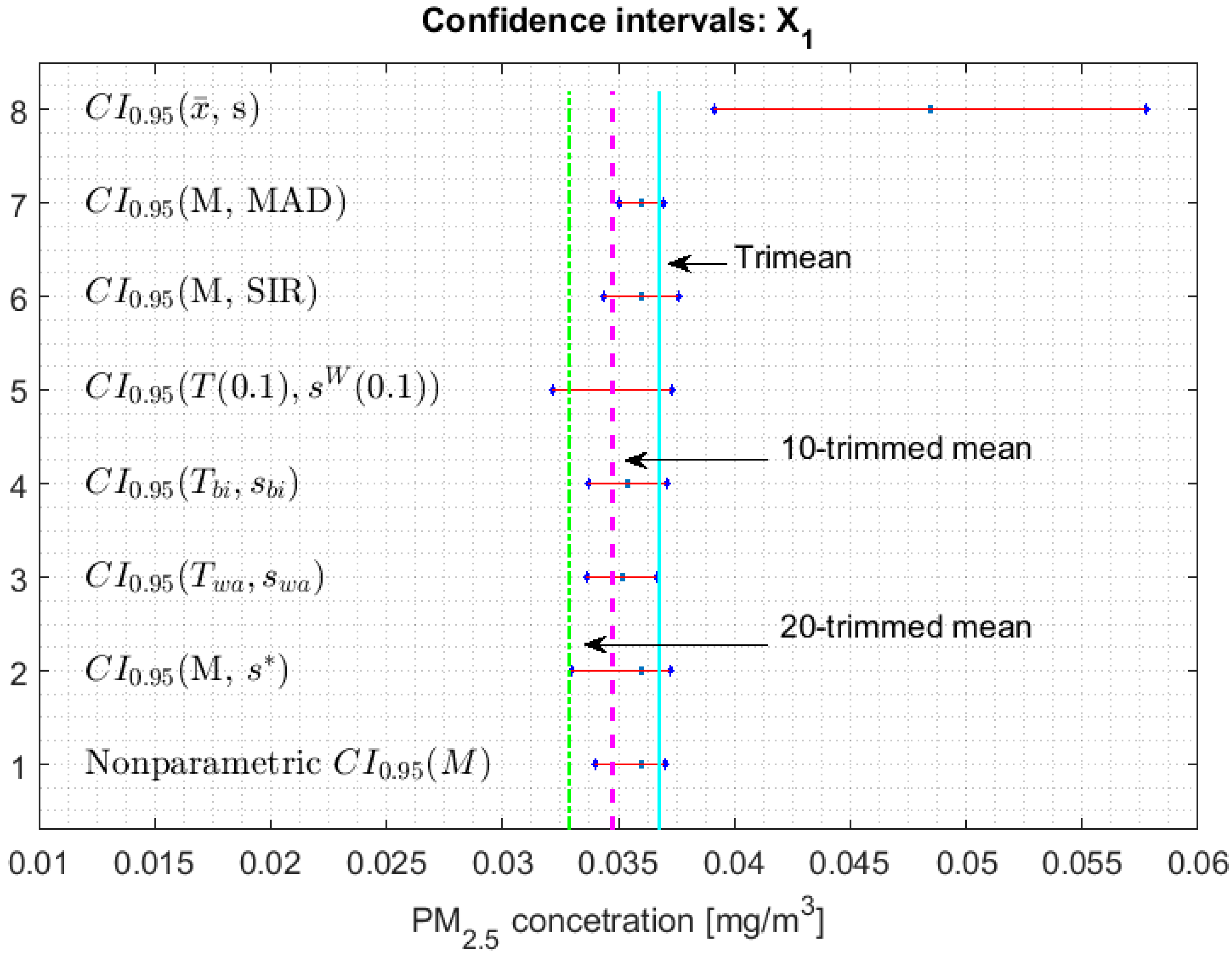
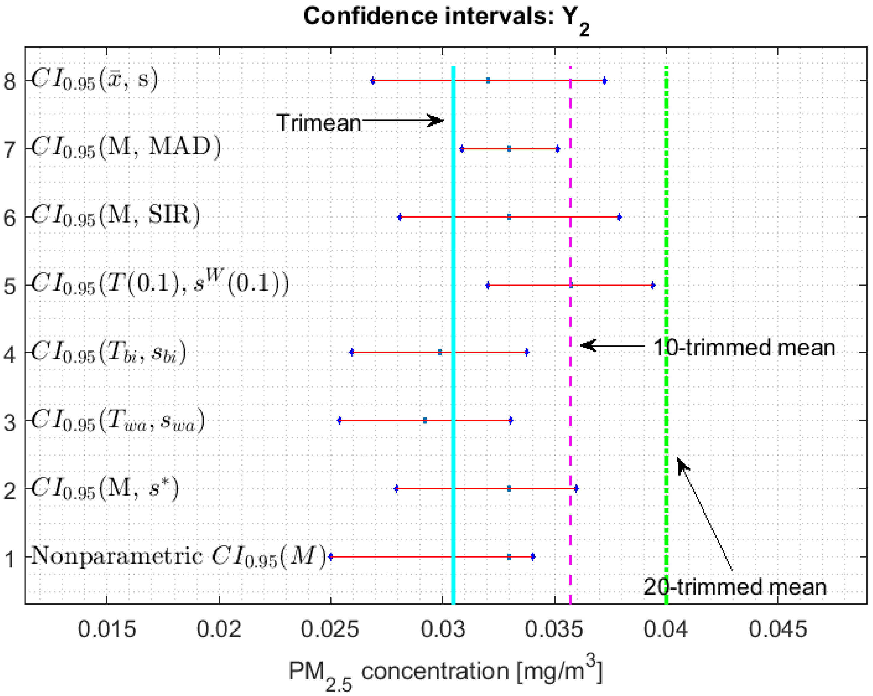
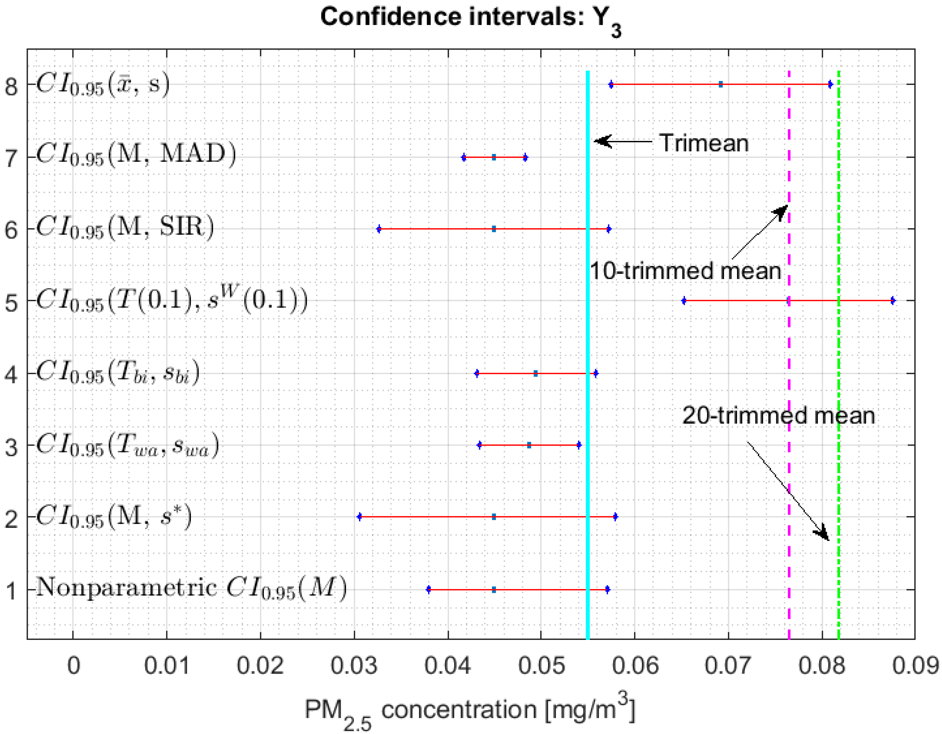
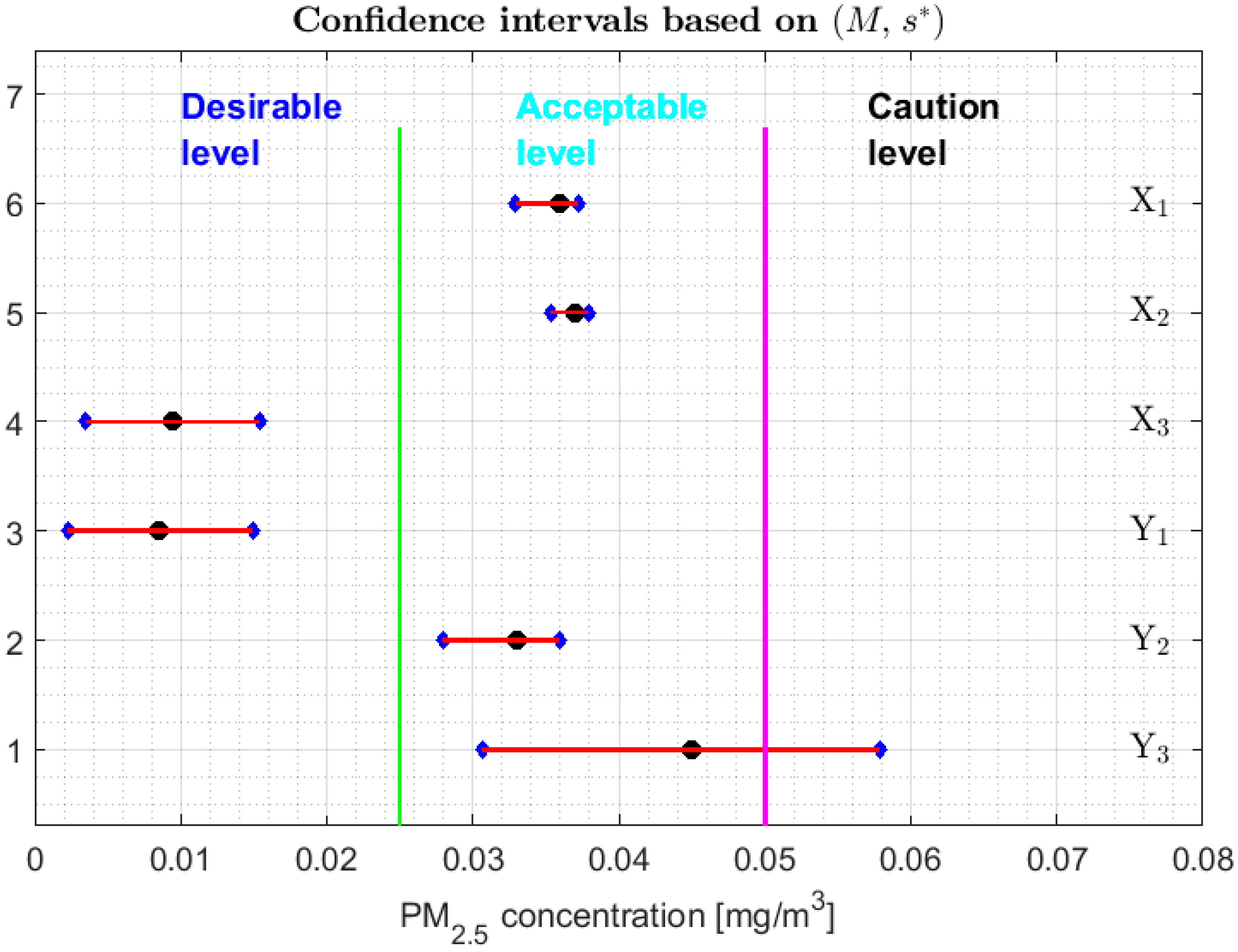
3.2. Confidence Interval for Each Parameter
- 1.
- One cannot reject that variables and can have equal medians, and, with a confidence level, it is rejected that they are the medians of any of the other variables, since the acceptance limits of the first two variables do not include the acceptance limits of the others.
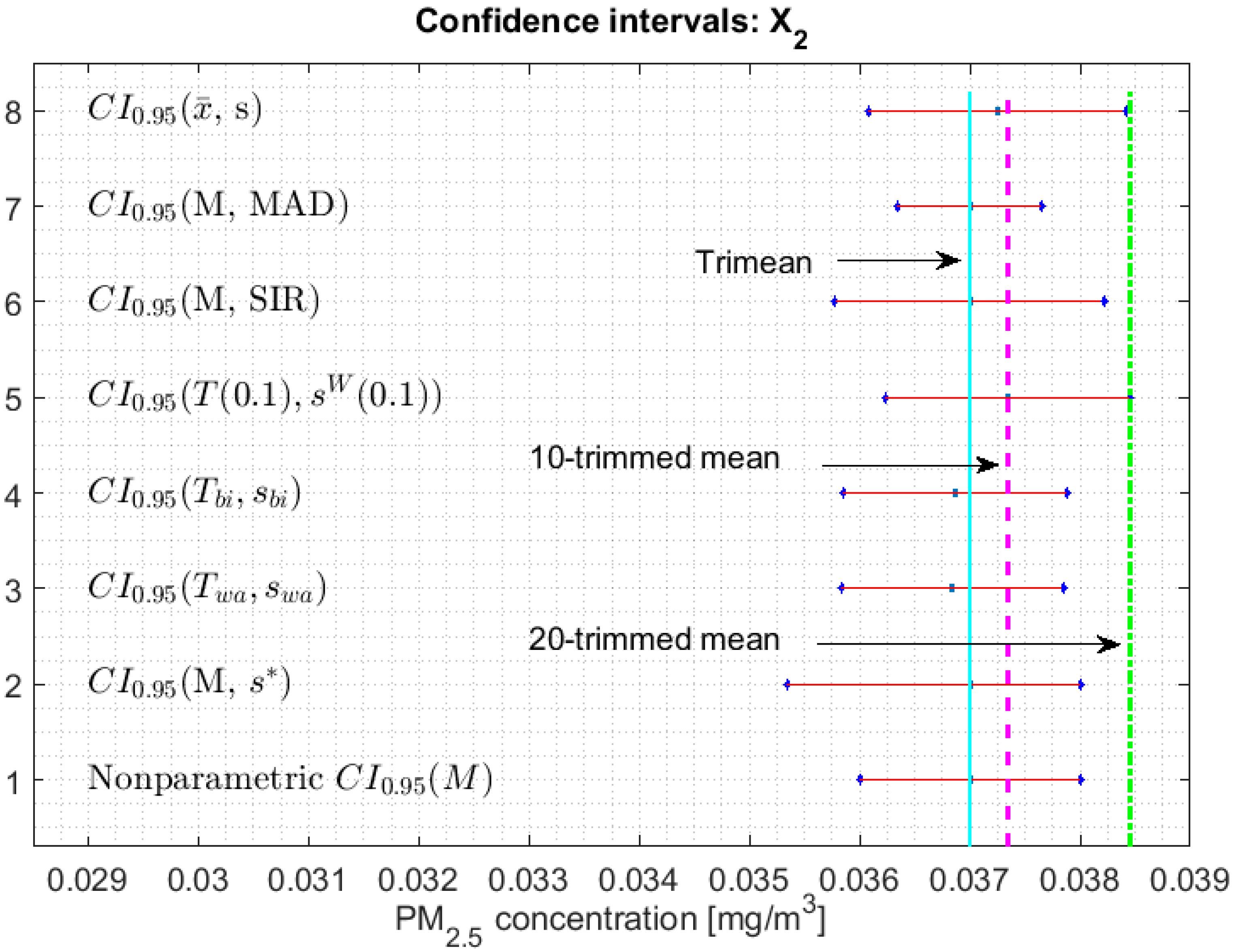
- 2.
- One cannot reject that the variables , , , and can have equal medians.
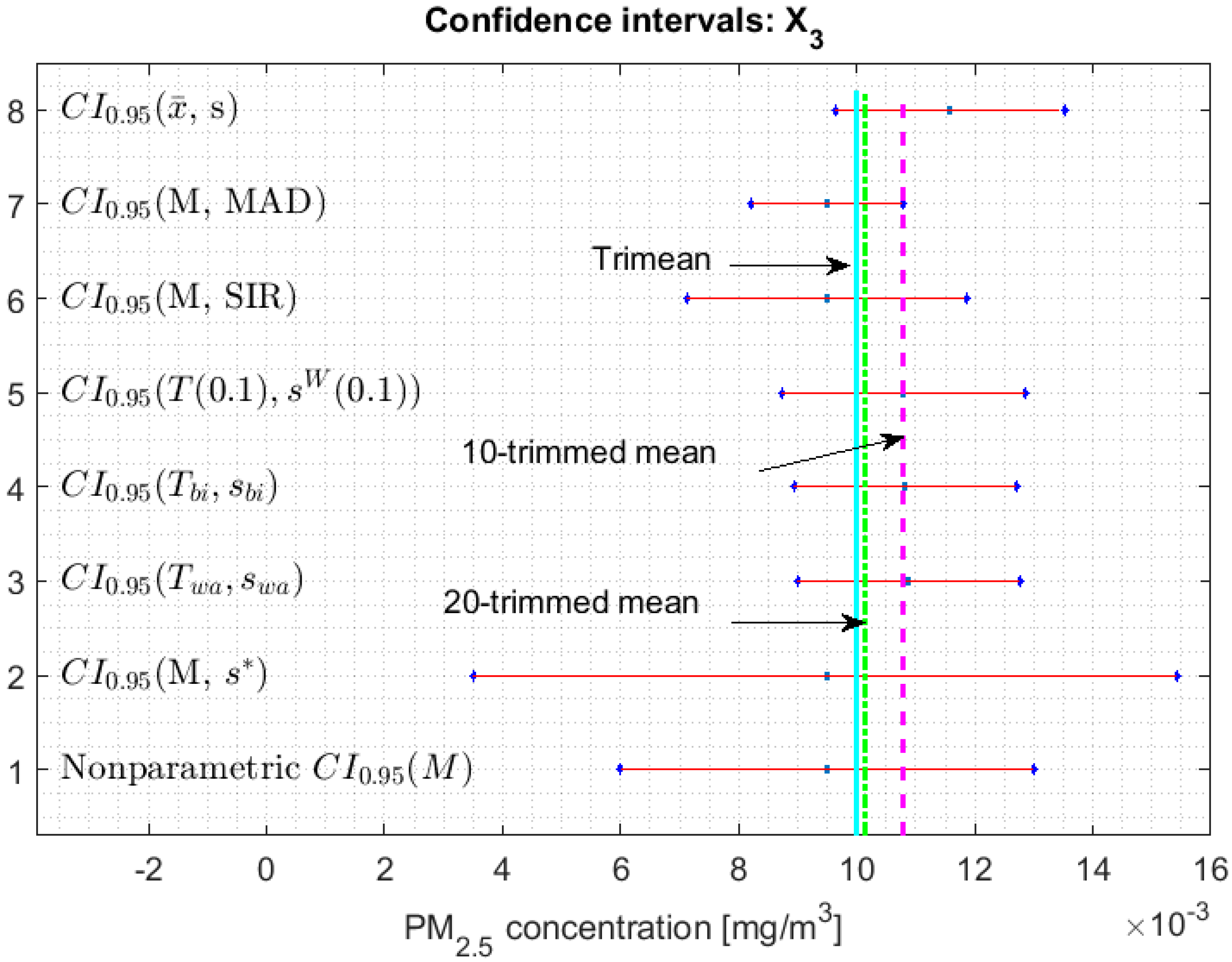
- 3.
- When removing the observations of the tails of the distributions, the variables and are those that present less variability, and the variables and have more variability than the rest.
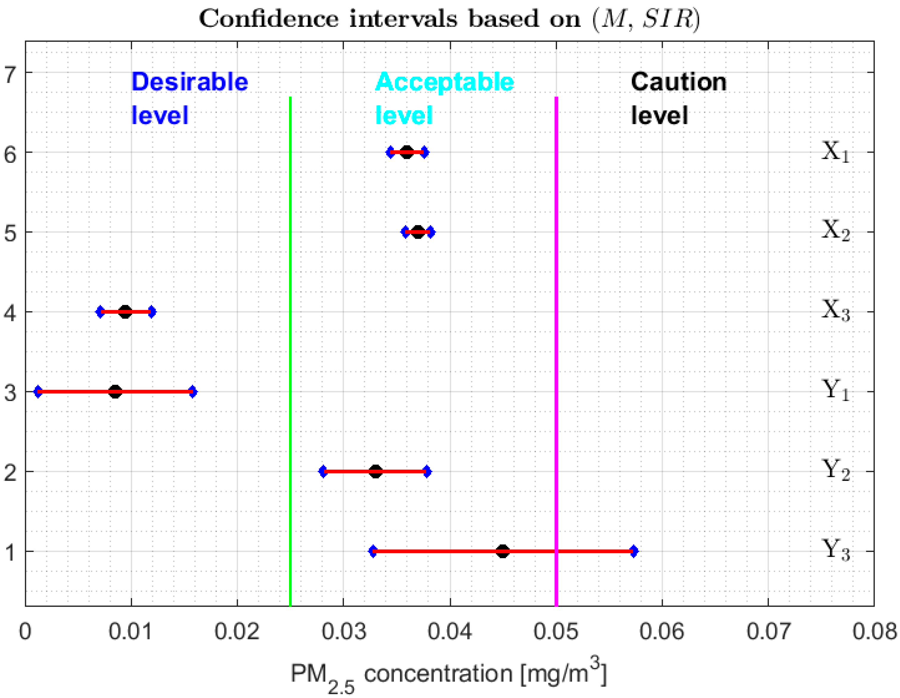
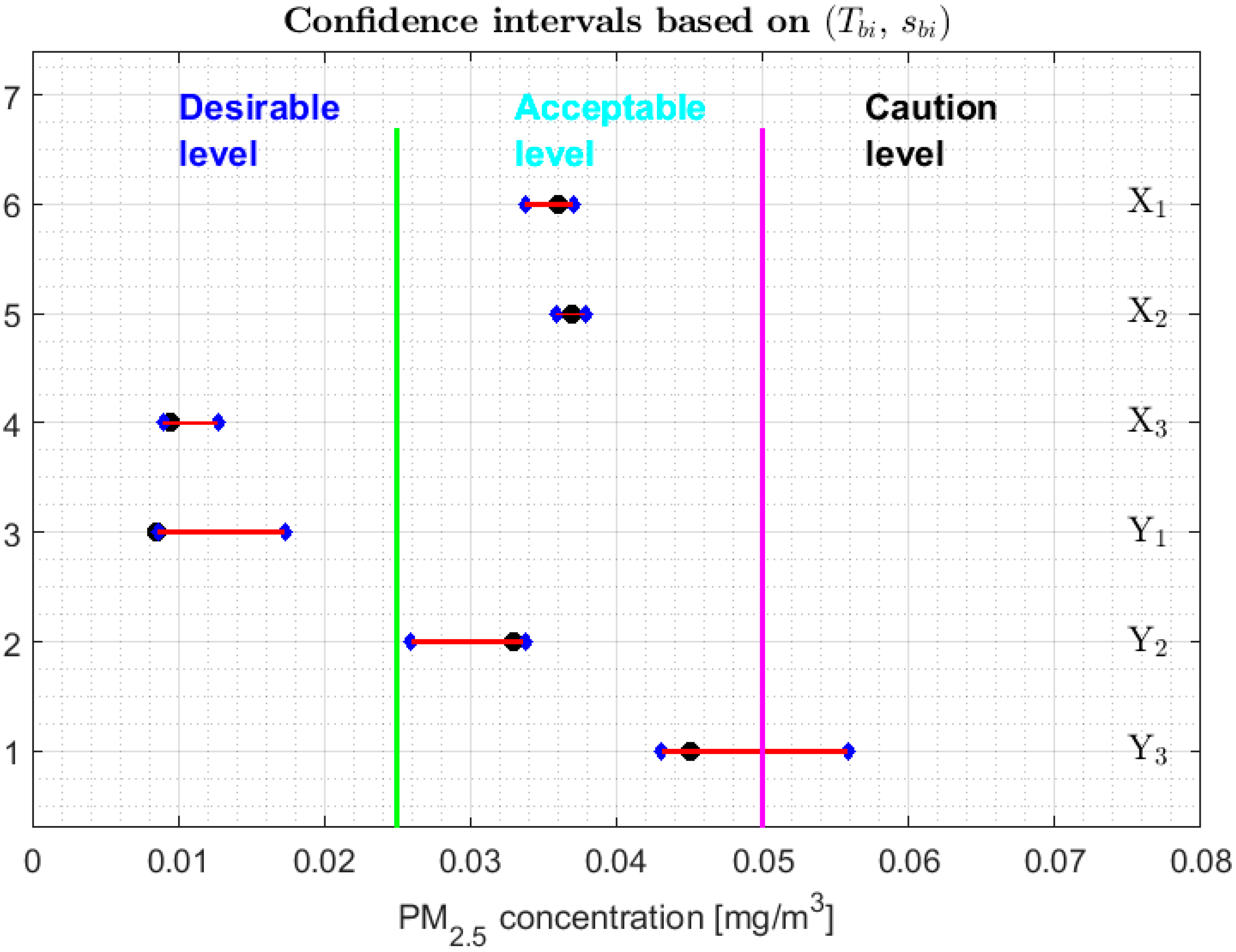
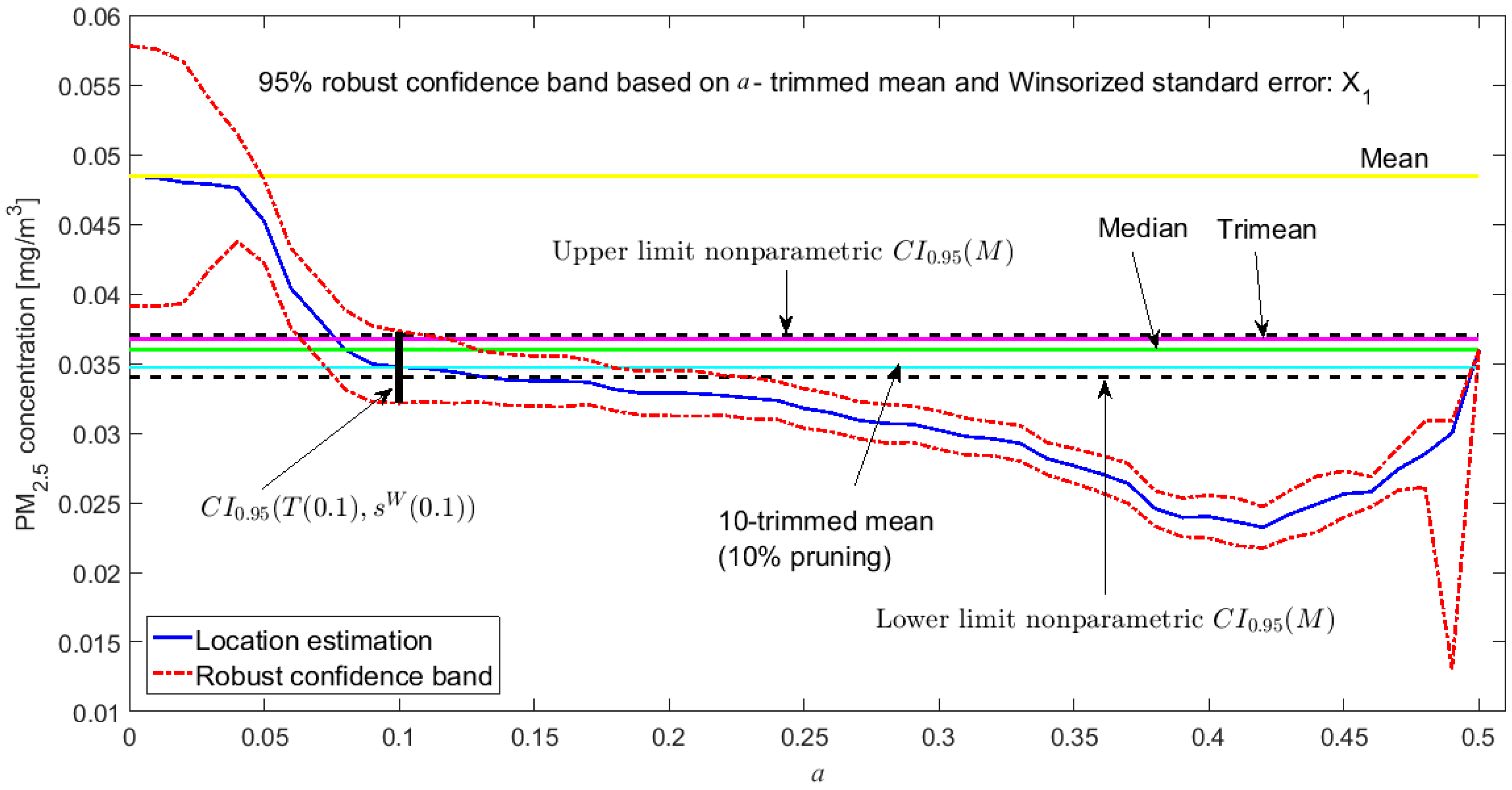
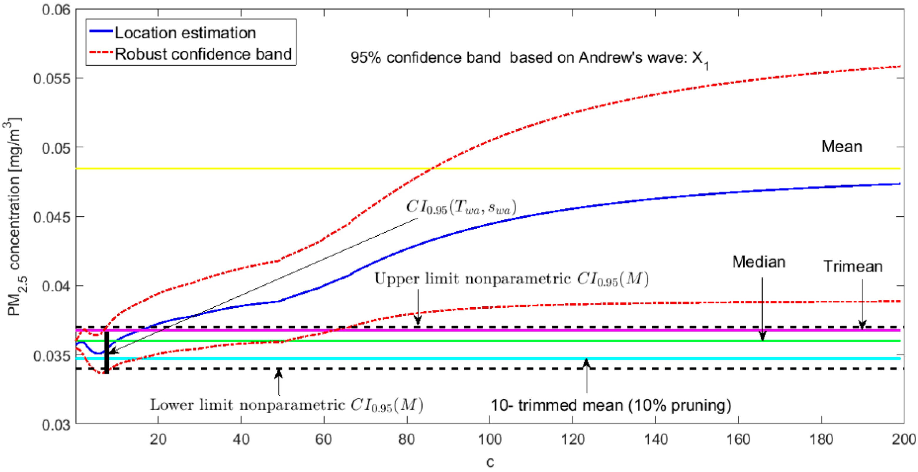
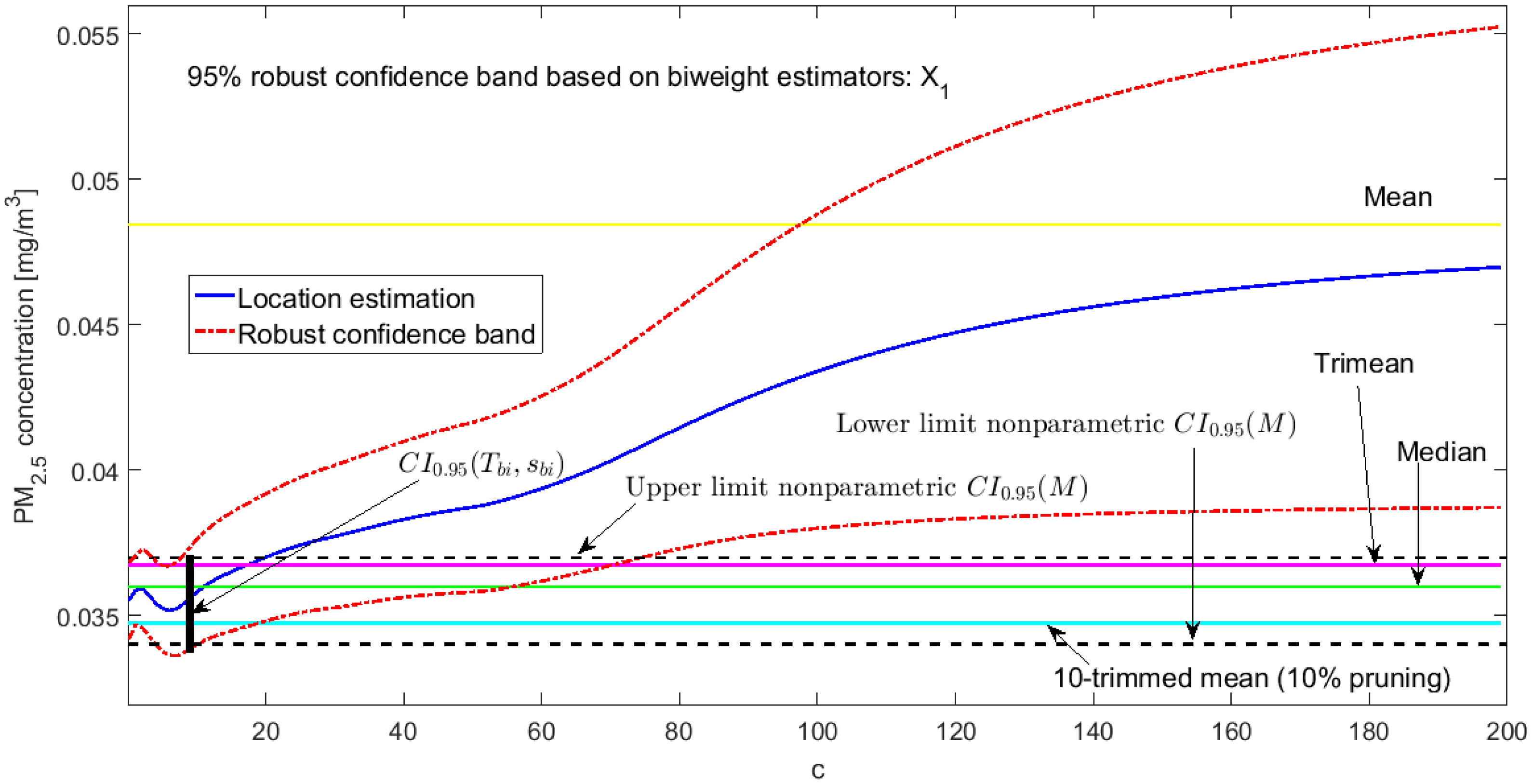
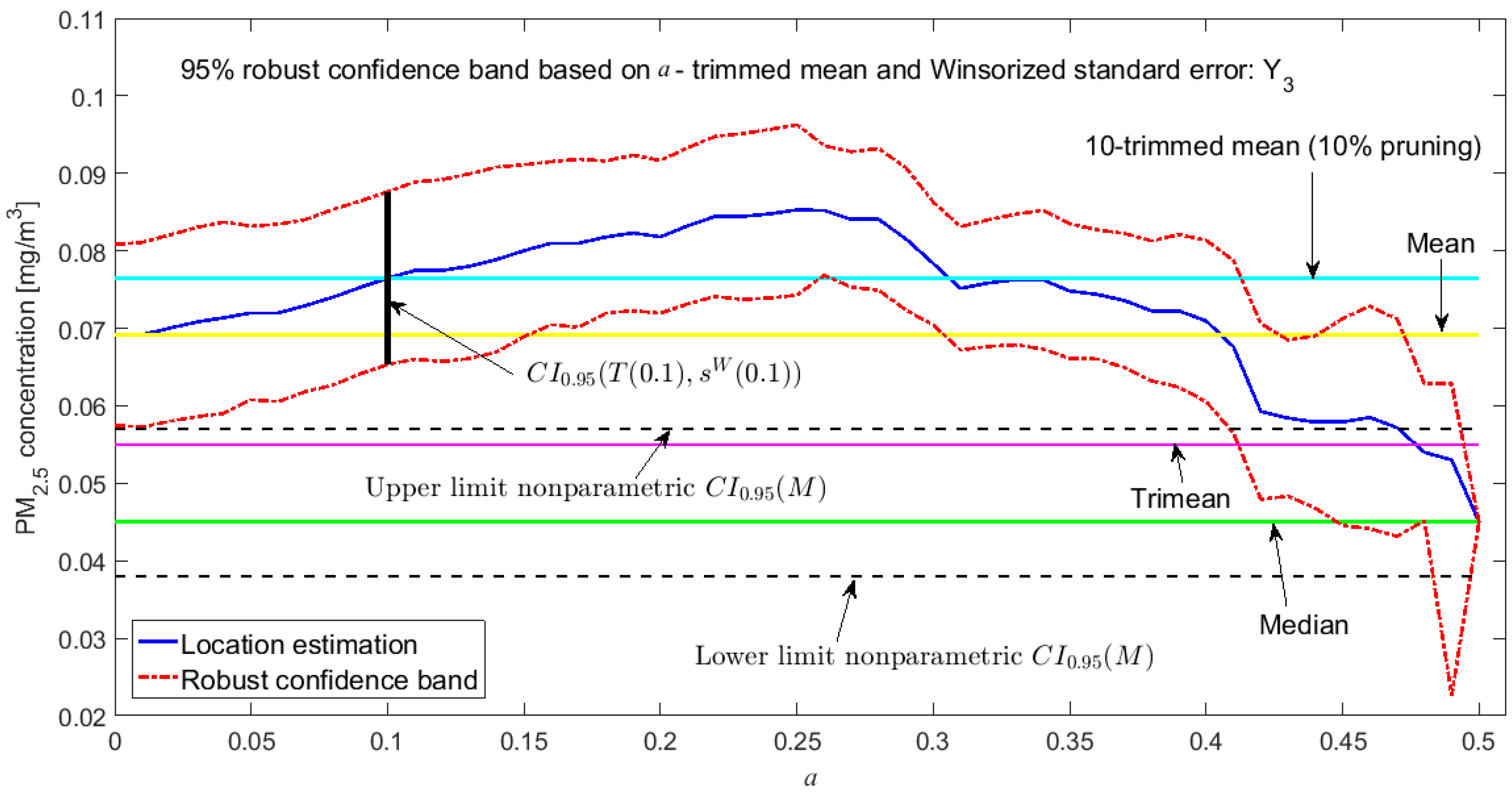
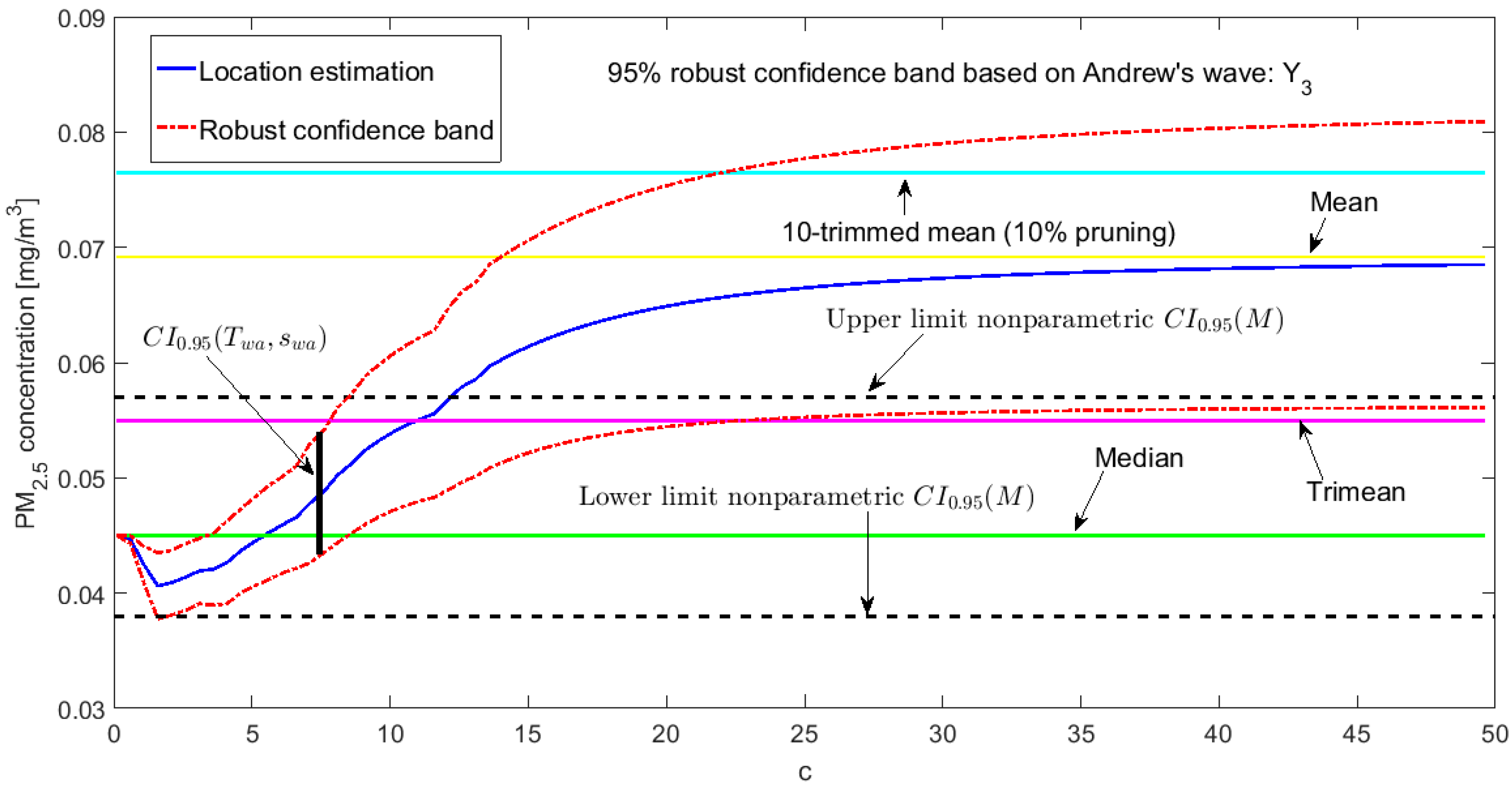
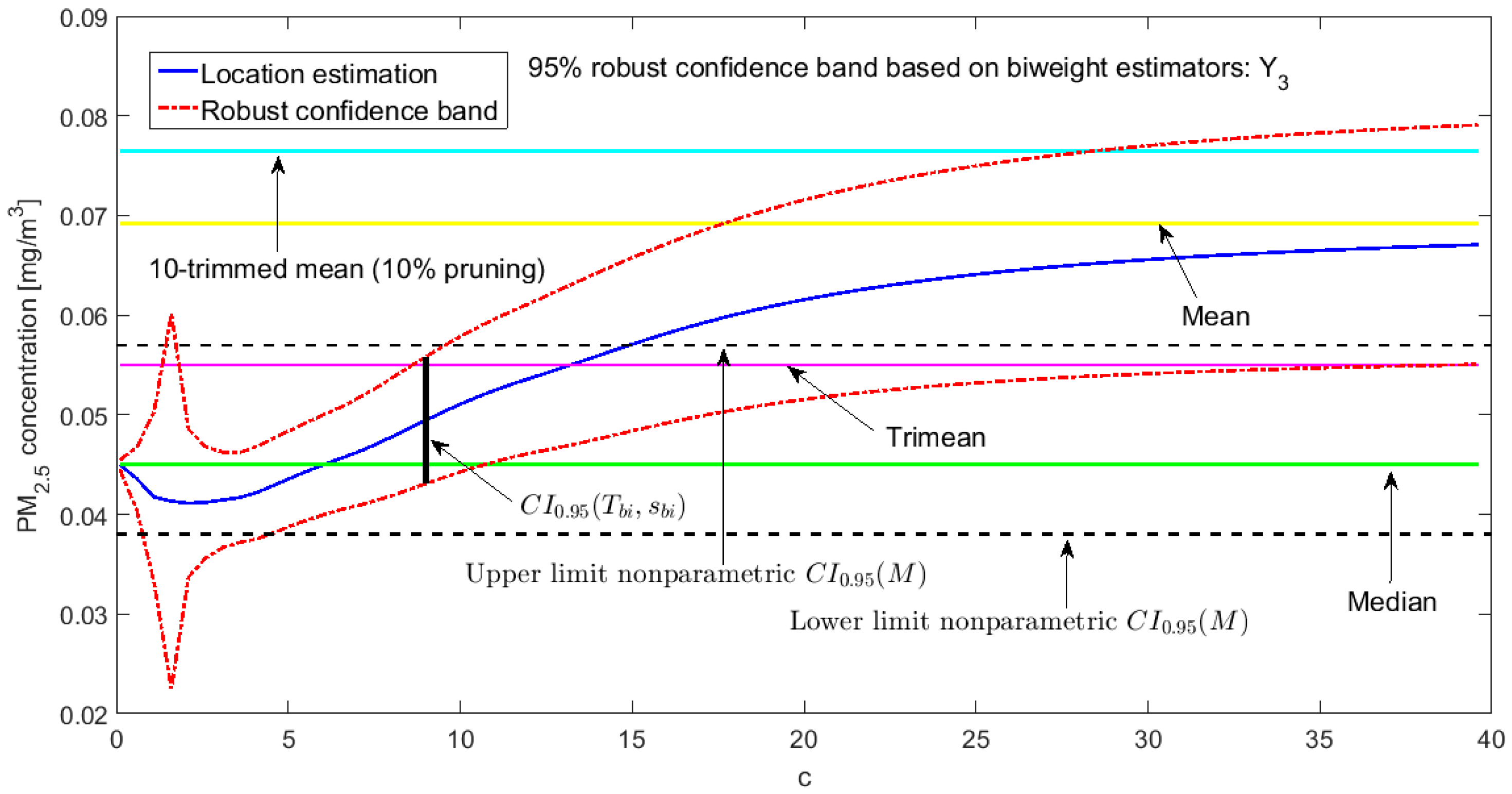
3.3. Robust Confidence Band Graphs
4. Conclusions
Author Contributions
Funding
Conflicts of Interest
References
- WHO. Health Aspects of Air Pollution with Particulate Matter, Ozone and Nitrogen Dioxide; Report on a WHO Working Group; WHO: Bonn, Germany, 2003; Available online: https://www.greenfacts.org/en/particulate-matter-pm/index.htm#1 (accessed on 4 December 2019).
- GreenFacts. Air Pollution Particulate Matter. Available online: https://www.greenfacts.org/en/particulate-matter-pm/level-2/01-presentation.htm#1 (accessed on 4 December 2019).
- Apte, J.S.; Brauer, M.; Cohen, A.J.; Ezzati, M.; Arden Pope, C., III. Ambient PM2.5 Reduces Global and Regional Life Expentancy. Environ. Sci. Technol. Lett. 2018, 5, 546–551. [Google Scholar] [CrossRef] [Green Version]
- Xing, Y.F.; Xu, Y.H.; Shi, M.H.; Lian, Y.X. The impact of PM2.5 on the human respiratory system. J. Thorac. Dis. 2016, 8, E69–E74. [Google Scholar] [PubMed]
- Samoli, E.; Analitis, A.; Touloumi, G.; Schwartz, J.; Anderson, H.R.; Sunyer, J.; Bisanti, L.; Zmirou, D.; Vonk, J.M.; Pekkanen, J.; et al. Estimating the Exposure-Response Relationships between Particulate Matter and Mortality within the APHEA Multicity Project. Environ. Health Perspect. 2005, 113, 88–95. [Google Scholar] [CrossRef] [PubMed]
- Ostro, B.; Broadwin, R.; Green, S.; Feng, W.Y.; Lipsett, M. Fine Particulate Air Pollution and Mortality in Nine California Counties: Results from CALFINE. Environ. Health Perspect. 2006, 114, 29–33. [Google Scholar] [CrossRef] [Green Version]
- Lewis, T.C.; Robins, T.G.; Dvonch, J.T.; Keeler, G.J.; Yip, F.Y.; Mentz, G.B.; Lin, X.; Parker, E.A.; Israel, B.A.; Gonzalez, L.; et al. Air Pollution-Associated Changes in Lung Function among Asthmatic Children in Detroit. Environ. Health Perspect. 2005, 113, 1068–1075. [Google Scholar] [CrossRef] [Green Version]
- Cao, Q.; Rui, G.; Liang, Y. Study on PM2.5 Pollution and the Mortality Due to Lung Cancer in China Based on Geographic Weighted Regression Model. BMC Public Health 2018, 18, 925–934. [Google Scholar] [CrossRef]
- Lim, J.M.; Jeong, J.H.; Lee, J.H.; Moon, J.H.; Chung, Y.S.; Kim, K.H. The Analysis of PM2.5 and Associated Elements and their Indoor/Outdoor Pollution Status in an Urban Area. Indoor Air 2011, 21, 145–155. [Google Scholar] [CrossRef]
- Van Donkelaar, A.; Martin, R.V.; Brauer, M.; Kahn, R.; Levy, R.; Verduzco, C.; Villeneuve, P.J. Global Estimates of Ambient Fine Particulate Matter Concentrations from Satellite-Based Aerosol Optical Depth: Development and Application. Environ. Health Perspect. 2010, 118, 847–855. [Google Scholar] [CrossRef] [Green Version]
- Ranft, U.; Schikowski, T.; Sugiri, D.; Krutmann, J.; Krämer, U. Long-Term Exposure to Traffic-Related Particulate Matter Impairs Cognitive Function in the Elderly. Environ. Res. 2009, 109, 1004–1011. [Google Scholar] [CrossRef]
- Hernandez, W.; Mendez, A.; Diaz-Marquez, A.M.; Zalakeviciute, R. PM2.5 Concentration Measurement Analysis by Using Non-Parametric Statistical Inference. IEEE Sens. J. 2020, 20, 1084–1094. [Google Scholar] [CrossRef]
- Hernandez, W.; Mendez, A.; Diaz-Marquez, A.M.; Zalakeviciute, R. Robust Analysis of PM2.5 Concentration Measurements in the Ecuadorian Park La Carolina. Sensors 2019, 19, 4648. [Google Scholar] [CrossRef] [PubMed] [Green Version]
- Hernandez, W.; Mendez, A.; Zalakeviciute, R.; Diaz-Marquez, A.M. Analysis of the information obtained from PM2.5 concentration measurements in an urban park. IEEE Trans. Instrum. Meas. 2020. [Google Scholar] [CrossRef]
- Qiu, L.; Liu, F.; Zhang, X.; Gao, T. The Reducing Effect of Green Spaces with Different Vegetation Structure on Atmospheric Particulate Matter Concentration in BaoJi City, China. Atmosphere 2018, 9, 332. [Google Scholar] [CrossRef] [Green Version]
- Jänhall, S. Review on Urban Vegetation and Particle Air Pollution - Deposition and Dispersion. Atmos. Environ. 2015, 105, 130–137. [Google Scholar] [CrossRef]
- Litschke, T.; Kuttler, W. On the Reduction of Urban Particle Concentration by Vegetation—A Review. Meteorol. Z. 2008, 17, 229–240. [Google Scholar] [CrossRef]
- Zupanic, T.; Westmacott, C.; Bulthuis, M. The Impact of Green Space on Heat and Air Pollution in Urban Communities: A Meta-Narrative Systematic Review; David Suzuki Fundation: Vancouver, BC, Canada, 2015; Available online: https://davidsuzuki.org/wp-content/uploads/2017/09/impact-greenspace-heat-air-pollution-urban-communities.pdf (accessed on 13 August 2019).
- Wang, Q.; Zeng, Q.; Tao, J.; Sun, L.; Zhang, L.; Gu, T.; Wang, Z.; Chen, L. Estimating PM2.5 Concentrations Based on MODIS AOD and NAQPMS Data over Beijing–Tianjin–Hebei. Sensors 2019, 19, 1207. [Google Scholar] [CrossRef] [PubMed] [Green Version]
- Reece, S.; Williams, R.; Colón, M.; Southgate, D.; Huertas, E.; O’Shea, M.; Iglesias, A.; Sheridan, P. Spatial-Temporal Analysis of PM2.5 and NO2 Concentrations Collected Using Low-Cost Sensors in Peñuelas, Puerto Rico. Sensors 2018, 18, 4314. [Google Scholar] [CrossRef] [Green Version]
- Mahajan, S.; Chen, L.J.; Tsai, T.C. Short-Term PM2.5 Forecasting Using Exponential Smoothing Method: A Comparative Analysis. Sensors 2018, 18, 3223. [Google Scholar] [CrossRef] [Green Version]
- Cavaliere, A.; Carotenuto, F.; Di Gennaro, F.; Gioli, B.; Gualtieri, G.; Martelli, F.; Matese, A.; Toscano, P.; Vagnoli, C.; Zaldei, A. Development of Low-Cost Air Quality Stations for Next Generation Monitoring Networks: Calibration and Validation of PM2.5 and PM10 Sensors. Sensors 2018, 18, 2843. [Google Scholar] [CrossRef] [Green Version]
- Genikomsakis, K.N.; Galatoulas, N.-F.; Dallas, P.I.; Ibarra, L.M.C.; Margaritis, D.; Ioakimidis, C.S. Development and On-Field Testing of Low-Cost Portable System for Monitoring PM2.5 Concentrations. Sensors 2018, 18, 1056. [Google Scholar] [CrossRef] [Green Version]
- Hoaglin, D.C.; Mosteller, F.; Tukey, J.W. Understanding Robust and Exploratory Data Analysis; John Wiley & Sons: Hoboken, NJ, USA, 2000. [Google Scholar]
- Maronna, R.A.; Martin, R.D.; Yohai, V.J. Robust Statistics: Theory and Methods; John Wiley & Sons: Chichester, UK, 2006. [Google Scholar]
- Wilcox, R. Introduction to Robust Estimation and Hypothesis Testing, 3rd ed.; Academic Press: Waltham, MA, USA, 2012. [Google Scholar]
- Gibbons, J.D.; Chakraborti, S. Nonparametric Statistical Inference, 4th ed.; Marcel Dekker: New York, NY, USA, 2003. [Google Scholar]
- Gibbons, J.D. Nonparametric Methods for Quantitative Analysis, 3rd ed.; American Sciences Press: New York, NY, USA, 1996. [Google Scholar]
- Brockwell, P.J.; Davis, R.A. Introduction to Time Series and Forecasting, 2nd ed.; Springer: New York, NY, USA, 2002. [Google Scholar]
- Paez, C.; Diaz, V. Reporte de Secretaría de Ambiente del Distrito Metropolitano de Quito. 2011. Available online: http://www.quitoambiente.gob.ec/ambiente/images/Secretaria_Ambiente/red_monitoreo/informacion/iqca.pdf (accessed on 7 August 2019).
- Hampel, F.R. The Influence Curve and its Role in Robust Estimation. J. Am. Stat. Assoc. 1974, 69, 383–393. [Google Scholar] [CrossRef]
- Croux, C.; Rouseeuw, P.J. A Class of High-Breakdown Scale Estimators Based on Subranges. Commun. Stat. Theory Methods 1992, 21, 1935–1951. [Google Scholar] [CrossRef]
- Mosteller, F.; Tukey, J.W. Data Analysis and Regression: A Second Course in Statistics; Addison-Wesley: Reading, MA, USA, 1977. [Google Scholar]
- Tukey, J.W.; McLaughlin, D.H. Less Vulnerable Confidence and Significance Procedures for Location Based on a Single Sample: Trimming/Winsorization 1. Sankhya Indian J. Stat. Ser. A 1963, 25, 331–352. [Google Scholar]


| Variable | ||||||
|---|---|---|---|---|---|---|
| Variable | ||||||
| Pair of Estimators | ||||||
|---|---|---|---|---|---|---|
| Nonparametric [13] | ||||||
© 2020 by the authors. Licensee MDPI, Basel, Switzerland. This article is an open access article distributed under the terms and conditions of the Creative Commons Attribution (CC BY) license (http://creativecommons.org/licenses/by/4.0/).
Share and Cite
Hernandez, W.; Mendez, A.; Zalakeviciute, R.; Diaz-Marquez, A.M. Robust Confidence Intervals for PM2.5 Concentration Measurements in the Ecuadorian Park La Carolina. Sensors 2020, 20, 654. https://doi.org/10.3390/s20030654
Hernandez W, Mendez A, Zalakeviciute R, Diaz-Marquez AM. Robust Confidence Intervals for PM2.5 Concentration Measurements in the Ecuadorian Park La Carolina. Sensors. 2020; 20(3):654. https://doi.org/10.3390/s20030654
Chicago/Turabian StyleHernandez, Wilmar, Alfredo Mendez, Rasa Zalakeviciute, and Angela Maria Diaz-Marquez. 2020. "Robust Confidence Intervals for PM2.5 Concentration Measurements in the Ecuadorian Park La Carolina" Sensors 20, no. 3: 654. https://doi.org/10.3390/s20030654