
The Community Structure of eDNA in the Los Angeles River Reveals an Altered Nitrogen Cycle at Impervious Sites
 , ,
, , 
Abstract
:1. Introduction
2. Materials and Methods
2.1. Sample Collection
2.2. DNA Isolation and Amplification

| Marker | Description | Target Organisms | Forward Primer | Reverse Primer | Reference |
|---|---|---|---|---|---|
| FITS | Fungal rRNA Internal Transcribed Spacer | Fungi | GTCGGTAAAACTCGTGCCAGC | CATAGTGGGGTATCTAATCCCAGTTTG | Yang et al., 2018 [21] |
| 16S | Prokaryotic rRNA small subunit | Bacteria, archaea | GTGYCAGCMGCCGCGGTAA | GGACTACNVGGGTWTCTAAT | F: 515F and R: 806R, see Caporaso et al., 2012 [22] |
| 18S | Eukaryotic rRNA small subunit | Fungi, algae, protists | GTACACACCGCCCGTC | TGATCCTTCTGCAGGTTCACCTAC | Amaral-Zettler et al., 2009 [23]; Euk_1391f and EukBr |
| CO1 | Mitochondrial cytochrome oxidase subunit I | Animals | ATGCGATACTTGGTGTGAAT | GACGCTTCTCCAGACTACAAT | Gu et al., 2013 [24] |
| 12S | Mitochondrial rRNA small subunit | Fish, birds, snakes, insects | GGWACWGGWTGAACWGTWTAYCCYCC | TANACYTCnGGRTGNCCRAARAAYCA | Leray et al., 2013 [25] |
| PITS | Plant rRNA Internal Transcribed Spacer | Plants | GGAAGTAAAAGTCGTAACAAGG | CAAGAGATCCGTTGTTGAAAGTT | F: ITS5, White et al., 1990 [26]; R: 5.8S, Epp et al., 2012 [27] |
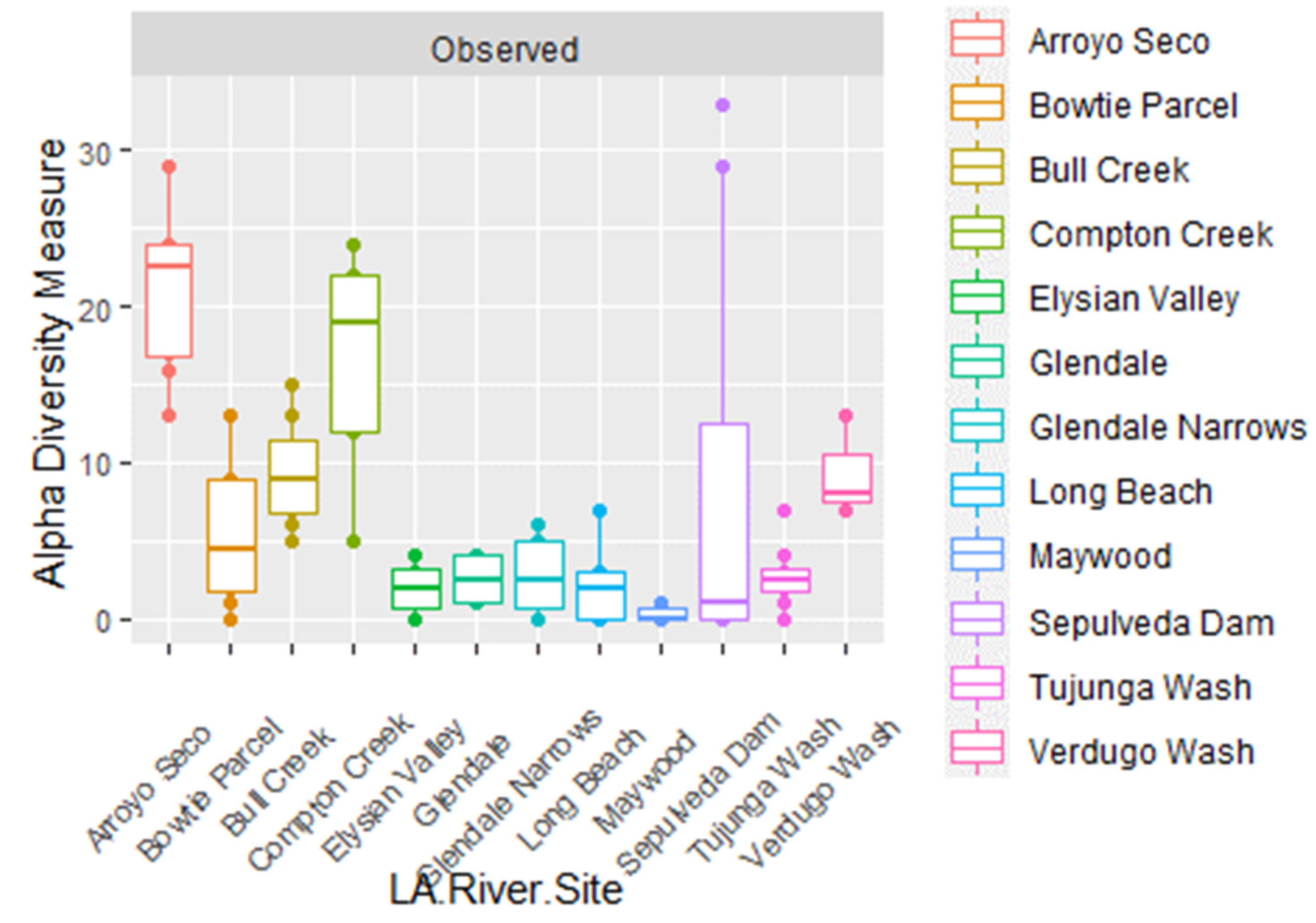
| Sample No. | LA River Site | Latitude | Longitude | Habitat | River Condition |
|---|---|---|---|---|---|
| K0585_T9 | Arroyo Seco | 34.203154 | −118.166402 | Frequently submerged, intertidal, marsh | soft |
| K0593_C3 | Arroyo Seco | 34.203274 | −118.166417 | Terrestrial, not submerged | soft |
| K0594_E4 | Arroyo Seco | 34.202987 | −118.166335 | Terrestrial, not submerged | soft |
| K0595_B2 | Arroyo Seco | 34.203593 | −118.166448 | Terrestrial, not submerged | soft |
| K0595_L7 | Arroyo Seco | 34.203567 | −118.166415 | Terrestrial, not submerged | soft |
| K0595_T9 | Arroyo Seco | 34.204139 | −118.166314 | Terrestrial, not submerged | soft |
| K0597_M8 | Arroyo Seco | 34.20375 | −118.166481 | Terrestrial, not submerged | soft |
| K0599_L7 | Arroyo Seco | 34.20331 | −118.166408 | Frequently submerged, intertidal, marsh | soft |
| K0526_B2 | Bowtie Parcel | 34.108161 | −118.246186 | Fully submerged | soft |
| K0529_L7 | Bowtie Parcel | 34.108149 | −118.246176 | Fully submerged | soft |
| K0672_C3 | Bowtie Parcel | 34.108433 | −118.246959 | Fully submerged | soft |
| K0672_G5 | Bowtie Parcel | 34.108278 | −118.246926 | Fully submerged | soft |
| K0674_E4 | Bowtie Parcel | 34.108186 | −118.246584 | Fully submerged | soft |
| K0678_E4 | Bowtie Parcel | 34.108131 | −118.246003 | Fully submerged | soft |
| K0679_B2 | Bowtie Parcel | 34.108278 | −118.246341 | Fully submerged | soft |
| K0679_M8 | Bowtie Parcel | 34.108374 | −118.246774 | Fully submerged | soft |
| K0528_A1 | Bull Creek | 34.181558 | −118.497717 | Frequently submerged, intertidal, marsh | soft |
| K0528_E4 | Bull Creek | 34.182029 | −118.49771 | Frequently submerged, intertidal, marsh | soft |
| K0528_K6 | Bull Creek | 34.181975 | −118.497849 | Frequently submerged, intertidal, marsh | soft |
| K0529_K6 | Bull Creek | 34.181652 | −118.497718 | Frequently submerged, intertidal, marsh | soft |
| K0529_T9 | Bull Creek | 34.181651 | −118.497716 | Fully submerged | soft |
| K0530_A1 | Bull Creek | 34.181419 | −118.497763 | Frequently submerged, intertidal, marsh | soft |
| K0530_B2 | Bull Creek | 34.181342 | −118.497657 | Frequently submerged, intertidal, marsh | soft |
| K0530_E4 | Bull Creek | 34.1814 | −118.497865 | Frequently submerged, intertidal, marsh | soft |
| K0528_G5 | Compton Creek | 33.843656 | −118.206466 | Frequently submerged, intertidal, marsh | soft |
| K0528_L7 | Compton Creek | 33.843055 | −118.205667 | Fully submerged | soft |
| K0528_T9 | Compton Creek | 33.843328 | −118.2061 | Frequently submerged, intertidal, marsh | soft |
| K0529_A1 | Compton Creek | 33.843196 | −118.205854 | Frequently submerged, intertidal, marsh | soft |
| K0530_C3 | Compton Creek | 33.843311 | −118.206092 | Frequently submerged, intertidal, marsh | soft |
| K0530_K6 | Compton Creek | 33.842877 | −118.205544 | Frequently submerged, intertidal, marsh | soft |
| K0530_L7 | Compton Creek | 33.842749 | −118.205402 | Fully submerged | soft |
| K0530_M8 | Compton Creek | 33.843196 | −118.205854 | Frequently submerged, intertidal, marsh | soft |
| K0529_C3 | Elysian Valley | 34.083829 | −118.228152 | Fully submerged | concrete |
| K0672_T9 | Elysian Valley | 34.084621 | −118.228071 | Frequently submerged, intertidal, marsh | concrete |
| K0673_A1 | Elysian Valley | 34.084217 | −118.228066 | Frequently submerged, intertidal, marsh | concrete |
| K0673_G5 | Elysian Valley | 34.084227 | −118.228048 | Fully submerged | concrete |
| K0674_G5 | Elysian Valley | 34.08455 | −118.228053 | Fully submerged | concrete |
| K0676_B2 | Elysian Valley | 34.08449 | −118.228157 | Fully submerged | concrete |
| K0676_T9 | Elysian Valley | 34.084721 | −118.228145 | Fully submerged | concrete |
| K0677_A1 | Elysian Valley | 34.084482 | −118.228157 | Frequently submerged, intertidal, marsh | concrete |
| K0593_T9 | Glendale | 34.155282 | −118.275211 | Fully submerged | concrete |
| K0594_L7 | Glendale | 34.15459 | −118.276618 | Fully submerged | concrete |
| K0596_C3 | Glendale | 34.155107 | −118.275459 | Fully submerged | concrete |
| K0596_E4 | Glendale | 34.154774 | −118.27637 | Frequently submerged, intertidal, mars | concrete |
| K0596_L7 | Glendale | 34.154918 | −118.276231 | Fully submerged | concrete |
| K0596_T9 | Glendale | 34.154973 | −118.275799 | Fully submerged | concrete |
| K0597_K6 | Glendale | 34.154997 | −118.275944 | Fully submerged | concrete |
| K0597_L7 | Glendale | 34.155157 | −118.27542 | Fully submerged | concrete |
| K0526_C3 | Glendale Narrows | 34.102813 | −118.242742 | Fully submerged | concrete |
| K0526_G5 | Glendale Narrows | 34.103427 | −118.242642 | Fully submerged | concrete |
| K0529_B2 | Glendale Narrows | 34.103109 | −118.242634 | Fully submerged | soft |
| K0529_G5 | Glendale Narrows | 34.103652 | −118.242686 | Fully submerged | concrete |
| K0529_M8 | Glendale Narrows | 34.103251 | −118.242645 | Fully submerged | concrete |
| K0672_B2 | Glendale Narrows | 34.10274 | −118.242669 | Fully submerged | concrete |
| K0678_B2 | Glendale Narrows | 34.103274 | −118.242544 | Fully submerged | concrete |
| K0678_K6 | Glendale Narrows | 34.103437 | −118.24275 | Fully submerged | concrete |
| K0672_A1 | Long Beach | 33.762909 | −118.202355 | Fully submerged | soft |
| K0674_M8 | Long Beach | 33.762738 | −118.202271 | Fully submerged | concrete |
| K0676_M8 | Long Beach | 33.762683 | −118.202126 | Fully submerged | concrete |
| K0677_B2 | Long Beach | 33.762833 | −118.202418 | Fully submerged | concrete |
| K0677_E4 | Long Beach | 33.762907 | −118.202298 | Fully submerged | concrete |
| K0677_L7 | Long Beach | 33.762841 | −118.20235 | Fully submerged | concrete |
| K0678_L7 | Long Beach | 33.762906 | −118.202305 | Fully submerged | soft |
| K0701_C3 | Long Beach | 33.76269 | −118.202303 | Fully submerged | concrete |
| K0527_A1 | Maywood | 33.986755 | −118.171412 | Frequently submerged, intertidal, marsh | concrete |
| K0527_C3 | Maywood | 33.988033 | −118.172607 | Fully submerged | concrete |
| K0527_E4 | Maywood | 33.987023 | −118.171842 | Fully submerged | concrete |
| K0527_K6 | Maywood | 33.986686 | −118.171342 | Fully submerged | concrete |
| K0527_L7 | Maywood | 33.987668 | −118.172288 | Fully submerged | concrete |
| K0527_T9 | Maywood | 33.986617 | −118.171324 | Fully submerged | concrete |
| K0539_L7 | Maywood | 33.986776 | −118.17165 | Fully submerged | concrete |
| K0593_G5 | Sepulveda Dam | 34.168961 | −118.475292 | Fully submerged | soft |
| K0594_A1 | Sepulveda Dam | 34.168698 | −118.475195 | Fully submerged | soft |
| K0594_T9 | Sepulveda Dam | 34.168961 | −118.475292 | Fully submerged | soft |
| K0595_G5 | Sepulveda Dam | 34.168941 | −118.47461 | Terrestrial, not submerged | soft |
| K0597_T9 | Sepulveda Dam | 34.1688 | −118.475049 | Fully submerged | soft |
| K0599_G5 | Sepulveda Dam | 34.16868 | −118.474846 | Frequently submerged, intertidal, marsh | soft |
| K0599_K6 | Sepulveda Dam | 34.168906 | −118.475125 | Fully submerged | soft |
| K0599_T9 | Sepulveda Dam | 34.168758 | −118.474733 | Rarely submerged, wetland, arroyo | soft |
| K0593_A1 | Tujunga Wash | 34.258032 | −118.386781 | Fully submerged | concrete |
| K0593_E4 | Tujunga Wash | 34.258403 | −118.386614 | Fully submerged | concrete |
| K0595_M8 | Tujunga Wash | 34.257481 | −118.386845 | Fully submerged | concrete |
| K0596_B2 | Tujunga Wash | 34.258667 | −118.386473 | Fully submerged | concrete |
| K0597_E4 | Tujunga Wash | 34.258716 | −118.386376 | Fully submerged | concrete |
| K0599_A1 | Tujunga Wash | 34.258424 | −118.386387 | Fully submerged | concrete |
| K0599_E4 | Tujunga Wash | 34.258395 | −118.386592 | Fully submerged | concrete |
| K0599_M8 | Tujunga Wash | 34.258016 | −118.386744 | Fully submerged | concrete |
| K0593_L7 | Verdugo Wash | 34.203216 | −118.237654 | Fully submerged | soft |
| K0595_A1 | Verdugo Wash | 34.202985 | −118.237755 | Fully submerged | soft |
| K0596_G5 | Verdugo Wash | 34.202611 | −118.237615 | Fully submerged | soft |
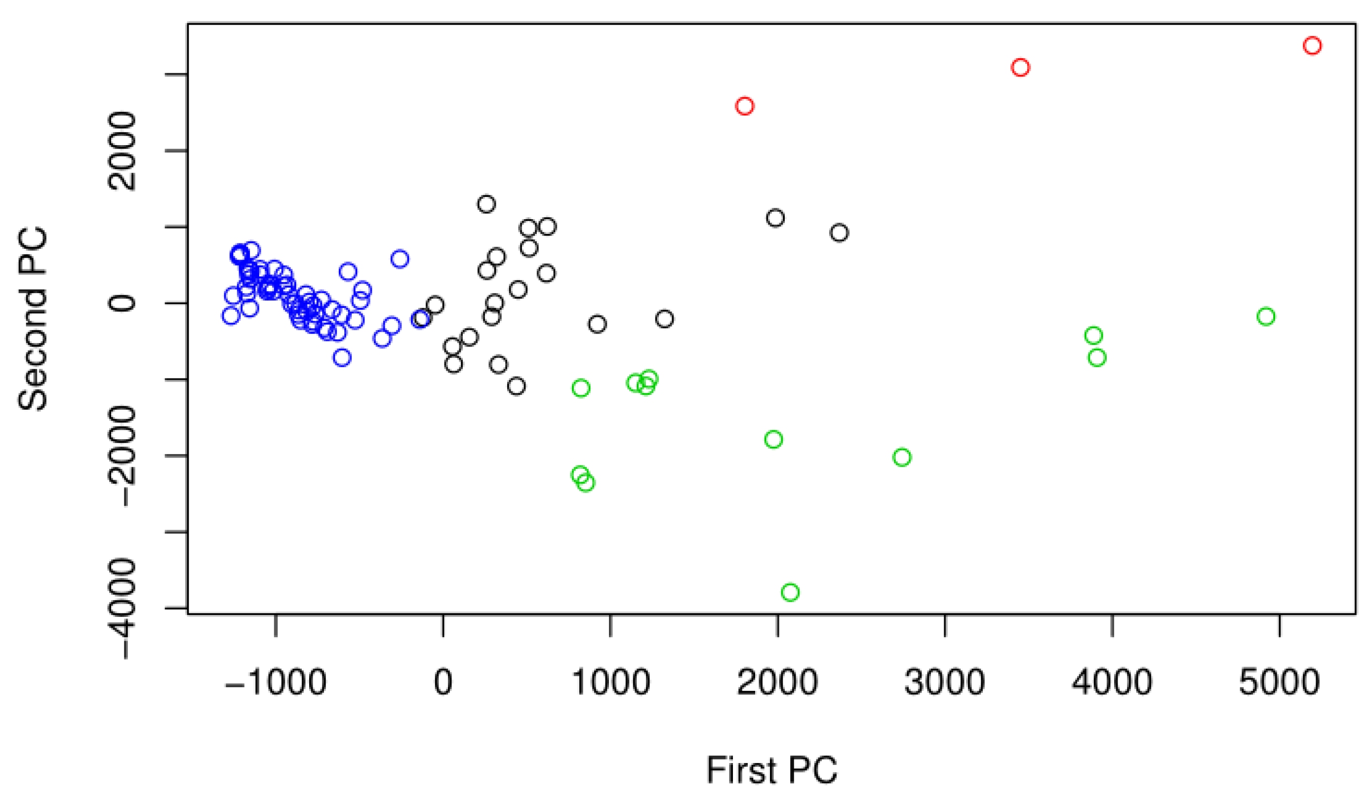
2.3. Statistical Approach
2.4. Chi Square Test of Proportions for the 18S Marker
2.5. Differential Abundance Analysis
- The mean parameter is the expectation value for Kij and is proportional to the actual number of sequence counts for gene i under the experimental condition ρ. The size factor is also accounted for, which is essentially the coverage or sequencing depth of the genetic library for each sample.
- The variance σ2 is the sum of the shot noise and the raw variance.
- The model uses a pooled variance from genes (or taxa) with similar count values to estimate the per gene raw variance.
- m size factors, including 1 for each sample.
- n expression strength parameters qip for each condition ρ. In other words, the expectation values for the abundance of counts for gene or taxon i are proportional to qip.
- The pooled variance parameter simulates the dependence of Vip on the expectation value for the mean, qip, for each condition ρ.
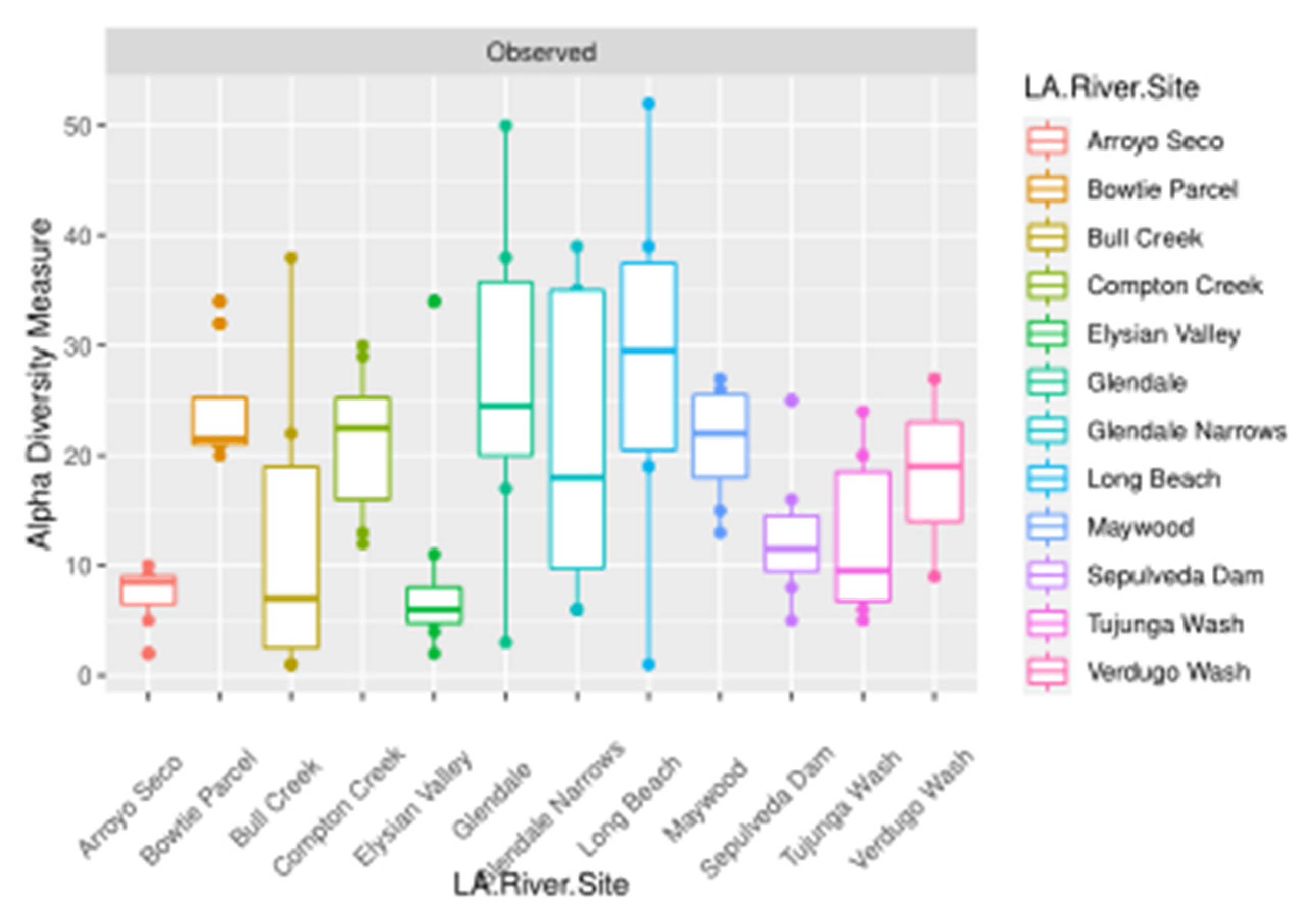
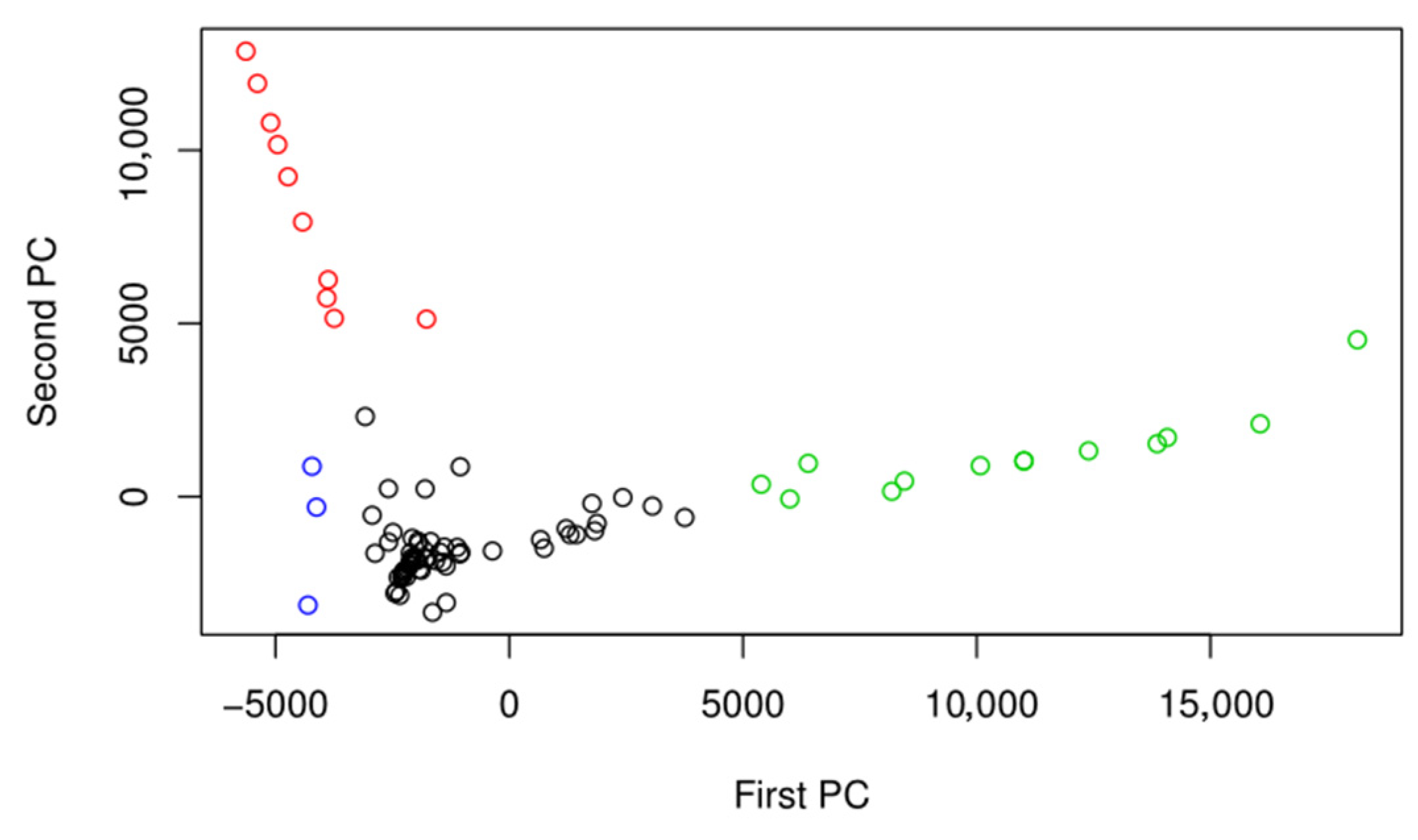
3. Results
4. Discussion
5. Conclusions
Supplementary Materials
Author Contributions
Funding
Institutional Review Board Statement
Data Availability Statement
Acknowledgments
Conflicts of Interest
References
- St. Louis Federal Reserve. Federal Reserve Economic Data. Available online: https://fred.stlouisfed.org/ (accessed on 3 April 2023).
- United States Census Bureau. Quick Facts: Los Angeles City, California. Available online: https://www.census.gov/quickfacts/losangelescitycalifornia (accessed on 3 April 2023).
- California Environmental Protection Board. Los Angeles River Watershed Impaired Waters. State Water Resources Control Board-Los Angeles. Available online: https://www.waterboards.ca.gov/rwqcb4/water_issues/programs/regional_program/Water_Quality_and_Watersheds/los_angeles_river_watershed/303.shtml (accessed on 6 July 2022).
- Protecting Our River. Available online: Protectingourriver.org (accessed on 17 October 2022).
- Qiu, H.; Gu, L.; Sun, B.; Zhang, J.; Zhang, M.; He, S.; An, S.; Leng, X. Metagenomic Analysis Revealed that the Terrestrial Pollutants Override the Effects of Seasonal Variation on Microbiome in River Sediments. Bull. Environ. Contam. Toxicol. 2020, 105, 892–898. [Google Scholar] [CrossRef] [PubMed]
- Wei, F.; Sakata, K.; Asakura, T.; Date, Y.; Kikuchi, J. Systemic Homeostasis in Metabolome, Ionome, and Microbiome of Wild Yellowfin Goby in Estuarine Ecosystem. Sci. Rep. 2018, 8, 3478. [Google Scholar] [CrossRef] [PubMed] [Green Version]
- Garba, F.; Ogidiaka, E.; Akamagwuna, F.C.; Nwaka, K.H.; Edegbene, O.A. Deteriorating water quality state on the structural assemblage of aquatic insects in a North-Western NigerianRiver. Water Sci. 2022, 36, 22–31. [Google Scholar] [CrossRef]
- Yuan, Q.; Wang, P.; Wang, C.; Chen, J.; Wang, X.; Liu, S. Indicator species and co-occurrence pattern of sediment bacterial community in relation to alkaline copper mine drainage contamination. Ecol. Indic. 2020, 120, 106884. [Google Scholar] [CrossRef]
- Khalilova, E.A.; Kotenko, S.T.; Islammagomedova, E.A.; Abakarova, A.A.; Chernyh, N.A.; Aliverdiyeva, D.A. Halophilic bacteria of salt lakes and saline soils of the Peri-Caspian lowland (Republic of Daghestan) and their biotechnological potential. Vavilov J. Genet. Breed. 2021, 25, 224–233. [Google Scholar] [CrossRef]
- Ackerman, D.; Schiff, K.; Trim, H.; Mullin, M. Characterization of water quality in the LA River. Bull. South. Calif. Acad. Sci. 2003, 102, 17–25. [Google Scholar]
- Desfor, G.; Keil, R. Every River Tells a Story: The Don River (Toronto) and the Los Angeles River (Los Angeles) as Articulating Landscapes. J. Environ. Policy Plan. 2000, 2, 5–23. [Google Scholar] [CrossRef]
- Gandy, M. Riparian anomie: Reflections on the Los Angeles River. Landsc. Res. 2006, 31, 135–145. [Google Scholar] [CrossRef]
- Wenger, S.J.; Roy, A.H.; Jackson, C.R.; Bernhardt, E.S.; Carter, T.L.; Filoso, S.; Gibson, C.A.; Hession, W.C.; Kaushal, S.S.; Martí, E.; et al. Twenty-six key research questions in urban stream ecology: An assessment of the state of the science. J. N. Am. Benthol. Soc. 2009, 28, 1080–1098. [Google Scholar] [CrossRef] [Green Version]
- Antwis, R.E.; Griffiths, S.; Harrison, X.; Bou, P.A.; Arce, A.; Bettridge, A.S.; Brailsford, F.; De Menezes, A.; Devaynes, A.; Forbes, K.M.; et al. Fifty important research questions in microbial ecology. FEMS Microbiol. Ecol. 2017, 93, fix044. [Google Scholar] [CrossRef]
- Orsi, J. Hazardous Metropolis: Flooding and Urban Ecology in Los Angeles; University of California Press: Berkeley, CA, USA, 2004; Available online: https://ebookcentral.proquest.com/lib/osu/detail.action?docID=227297 (accessed on 14 February 2023).
- Halecki, W.; Tomasz, S. Evaluation of Soil Hydrophysical Parameters Along a Semiurban Small River; Soil Ecosystem Services for Enhancing Water Retention in Urban and Suburban Green Areas. Catena 2022, 196, 104910. [Google Scholar] [CrossRef]
- Behera, B.K.; Patra, B.; Chakraborty, H.J.; Sahu, P.; Rout, A.K.; Sarkar, D.J.; Parida, P.K.; Raman, R.K.; Rao, A.R.; Rai, A.; et al. Metagenome analysis from the sediment of river Ganga and Yamuna: In search of beneficial microbiome. PLoS ONE 2020, 15, e0239594. [Google Scholar] [CrossRef]
- Caporaso, J.G.; Kuczynski, J.; Stombaugh, J.; Bittinger, K.; Bushman, F.D.; Costello, E.K.; Fierer, N.; Gonzalez Peña, A.; Goodrich, J.K.; Gordon, J.I.; et al. QIIME allows analysis of high-throughput community sequencing data. Nat. Methods 2010, 7, 335–336. [Google Scholar] [CrossRef] [Green Version]
- Curd, E.E.; Gold, Z.; Kandlikar, G.S.; Gomer, J.; Ogden, M.; O’Connell, T.; Pipes, L.; Schweizer, T.M.; Rabichow, L.; Lin, M.; et al. Anacapa Toolkit: An environmental DNA toolkit for processing multilocus metabarcode datasets. Methods Ecol. Evol. 2019, 10, 1469–1475. [Google Scholar] [CrossRef] [Green Version]
- Baragaño, B.; Ratié, R.; Sierra, C.; Chrastný, V.; Komárek, K.; Gallego, J. Multiple pollution sources unravelled by environmental forensics techniques and multivariate statistics. J. Hazard. Mater. 2021, 424, 127413. [Google Scholar] [CrossRef] [PubMed]
- Yang, R.H.; Su, J.H.; Shang, J.J.; Wu, Y.Y.; Li, Y.; Bao, D.P.; Yao, Y.J. Evaluation of the ribosomal DNA internal transcribed spacer (ITS), specifically ITS1 and ITS2, for the analysis of fungal diversity by deep sequencing. PLoS ONE 2018, 13, e0206428. [Google Scholar] [CrossRef] [PubMed] [Green Version]
- Caporaso, J.G.; Lauber, C.L.; Walters, W.A.; Berg-Lyons, D.; Huntley, J.; Fierer, N.; Owens, S.M.; Betley, J.; Fraser, L.; Bauer, M.; et al. Ultra-high-throughput microbial community analysis on the Illumina HiSeq and MiSeq platforms. ISME J. 2012, 6, 1621–1624. [Google Scholar] [CrossRef] [PubMed] [Green Version]
- Amaral-Zettler, L.A.; McCliment, E.A.; Ducklow, H.W.; Huse, S.M. A method for studying protistan diversity using massively parallel sequencing of V9 hypervariable regions of small-subunit ribosomal RNA genes. PLoS ONE 2009, 4, e6372. [Google Scholar] [CrossRef]
- Gu, W.; Song, J.; Cao, Y.; Sun, Q.; Yao, H.; Wu, Q.; Chao, J.; Zhou, J.; Xue, W.; Duan, J. Application of the ITS2 Region for Barcoding Medicinal Plants of Selaginellaceae in Pteridophyta. PLoS ONE 2013, 8, e67818. [Google Scholar] [CrossRef] [PubMed] [Green Version]
- Leray, M.; Yang, J.Y.; Meyer, C.P.; Mills, S.C.; Agudelo, N.; Ranwez, V.; Boehm, J.T.; Machida, R.J. A new versatile primer set targeting a short fragment of the mitochondrial COI region for metabarcoding metazoan diversity: Application for characterizing coral reef fish gut contents. Front. Zool. 2013, 10, 14–34. [Google Scholar] [CrossRef] [Green Version]
- White, T.J.; Bruns, T.; Lee, S.; Taylor, J. Amplification and direct sequencing of fungal ribosomal RNA genes for phylogenetics. In PCR Protocols: A Guide to Methods and Application; Innis, M.A., Gelfand, D.H., Sninsk, J.J., White, T.J., Eds.; Academic Press: San Diego, CA, USA, 1990; pp. 315–322. [Google Scholar]
- Epp, L.S.; Boessenkool, S.; Bellemain, E.P.; Haile, J.; Esposito, A.; Riaz, T.; Erséus, C.; Gusarov, V.I.; Edwards, M.E.; Johnsen, A.; et al. New environmental metabarcodes for analysing soil DNA: Potential for studying past and present ecosystems. Mol. Ecol. 2012, 21, 1821–1833. [Google Scholar] [CrossRef] [PubMed]
- Borg, I.; Groenen, P. Modern Multidimensional Scaling. Theory and Applications; Springer: Berlin/Heidelberg, Germany, 1997. [Google Scholar]
- Hastie, T.; Friedman, J. The Elements of Statistical Learning (ESL), 2nd ed.; Springer: Berlin/Heidelberg, Germany, 2009. [Google Scholar]
- McMurdie, P.J.; Holmes, S. phyloseq: An R Package for Reproducible Interactive Analysis and Graphics of Microbiome Census Data. PLoS ONE 2013, 8, e61217. [Google Scholar] [CrossRef] [PubMed] [Green Version]
- Kandlikar, G.S.; Gold, Z.; Cowen, M.C.; Meyer, R.S.; Freise, A.C.; Kraft, N.J.; Moberg-Parker, J.; Sprague, J.; Kushner, D.J.; Curd, E.E. ranacapa: An R package and Shiny web app to explore environmental DNA data with exploratory statistics and interactive visualizations. F1000Research 2018, 7, 1734. [Google Scholar] [CrossRef] [PubMed]
- Schubert, E.; Rousseeuw, P.J. Fast and eager k-medoids clustering: O (k) runtime improvement of the PAM, CLARA, and CLARANS algorithms. Inf. Syst. 2021, 101, 101804. [Google Scholar] [CrossRef]
- Lepère, C.; Domaizon, I.; Humbert, J.-F.; Jardillier, L.; Hugoni, M.; Debroas, D. Diversity, spatial distribution and activity of fungi in freshwater ecosystems. PeerJ 2019, 7, e6247. [Google Scholar] [CrossRef] [PubMed]
- Anders, S.; Huber, W. Differential expression analysis for sequence count data. Genome Biol. 2010, 11, R106. [Google Scholar] [CrossRef] [Green Version]
- Backman, T.W.H.; Girke, T. systemPipeR: NGS workflow and report generation environment. BMC Bioinform. 2016, 17, 388. [Google Scholar] [CrossRef] [Green Version]
- Blighe, K.; Rana, S.; Lewis, M. EnhancedVolcano: Publication-Ready Volcano Plots with Enhanced Colouring and Labeling; R Package Version 1.10.0; 2021; Available online: https://github.com/kevinblighe/EnhancedVolcano (accessed on 30 March 2023).
- Maria, L.; Andrés, P. Chapter Eleven-Aminoacyl-tRNA synthetases as drug targets. In The Enzymes; de Pouplana, L.R., Kaguni, L.S., Eds.; Academic Press: Cambridge, MA, USA, 2020; Volume 48, pp. 321–350. ISBN 9780128202609. ISSN 1874-6047. [Google Scholar] [CrossRef]
- Hanada, S. The Phylum Chloroflexi, the Family Chloroflexaceae, and the Related Phototrophic Families Oscillochloridaceae and Roseiflexaceae. In The Prokaryotes; Rosenberg, E., DeLong, E.F., Lory, S., Stackebrandt, E., Thompson, F., Eds.; Springer: Berlin/Heidelberg, Germany, 2014. [Google Scholar] [CrossRef]
- Willison, J.C.; Magnin, J.-P. Chapter Eight-Role and Evolution of Endogenous Plasmids in Photosynthetic Bacteria. In Advances in Botanical Research; Thomas Beatty, J., Ed.; Academic Press: Cambridge, MA, USA, 2013; Volume 66, pp. 227–265. ISSN 0065-2296. ISBN 9780123979230. [Google Scholar] [CrossRef]
- Teneva, I.; Dzhambazov, B.; Koleva, L.; Mladenov, R.; Schirmer, K. Toxic potential of five freshwater Phormidium species (Cyanoprokaryota). Toxicon 2005, 45, 711–725. [Google Scholar] [CrossRef]
- Synechococcus. Microbewiki, Kenyon College. Available online: https://microbewiki.kenyon.edu/index.php/Synechococcus (accessed on 1 April 2023).
- Oliveira, C.Y.B.; Oliveira, C.D.L.; Prasad, R.; Ong, H.C.; Araujo, E.S.; Shabnam, N.; Gálvez, A.O. A multidisciplinary review of Tetradesmus obliquus: A microalga suitable for large-scale biomass production and emerging environmental applications. Rev. Aquac. 2021, 13, 1594–1618. [Google Scholar] [CrossRef]
- Gouveia, L.; Jazić, J.M.; Ferreira, A.; Maletić, S.; Cvetković, D.; Vidović, S.; Vladi, J.Ć. Green approach for the valorization of microalgae Tetradesmus obliquus. Sustain. Chem. Pharm. 2021, 24, 100556. [Google Scholar] [CrossRef]
- Montclair State University. Microcystis. New Jersey Center for Water Science and Technology. Available online: https://www.montclair.edu/water-science/freshwater-cyanobacteria-of-new-jersey/visual-guide-to-cyanobacteria-in-new-jersey/coccoid/colonial/microcystis/ (accessed on 3 July 2022).
- Chroococcus. Microbewiki, Kenyon College. Available online: https://microbewiki.kenyon.edu/index.php/Chroococcus#Cell_Structure_and_Metabolism (accessed on 14 February 2023).
- Lucena, T.; Pascual, J.; Garay, E.; Arahal, D.R.; Macián, M.C.; Pujalte, M.J. Haliea mediterranea sp. nov., a marine gammaproteobacterium. Int. J. Syst. Evol. Microbiol. 2010, 60, 1844–1848. [Google Scholar] [CrossRef] [PubMed]
- Yang, L.; Tan, Z.; Wang, D.; Xue, L.; Guan, M.-X.; Huang, T.; Li, R. Species identification through mitochondrial rRNA genetic analysis. Sci. Rep. 2014, 4, 4089. [Google Scholar] [CrossRef] [PubMed] [Green Version]
- Kasozi, N.; Kaiser, H.; Wilhelmi, B. Metabarcoding Analysis of Bacterial Communities Associated with Media Grow Bed Zones in an Aquaponic System. Int. J. Microbiol. 2020, 2020, 8884070. [Google Scholar] [CrossRef] [PubMed]
- Islam, T.; Hernández, M.; Gessesse, A.; Murrell, J.C.; Øvreås, L. A Novel Moderately Thermophilic Facultative Methylotroph within the Class Alphaproteobacteria. Microorganisms 2021, 9, 477. [Google Scholar] [CrossRef] [PubMed]
- Jung, M.-Y.; Islam, A.; Gwak, J.-H.; Kim, J.-G.; Rhee, S.-K. Nitrosarchaeum koreense gen. nov., sp. nov., an aerobic and mesophilic, ammonia-oxidizing archaeon member of the phylum Thaumarchaeota isolated from agricultural soil. Int. J. Syst. Evol. Microbiol. 2018, 68, 3084–3095. [Google Scholar] [CrossRef] [PubMed]
- Pascual, J.; Foesel, B.; Geppert, A.; Huber, K.J.; Boedeker, C.; Luckner, M.; Wanner, G.; Overmann, J. Roseisolibacter agri gen. nov., sp. nov., a novel slow-growing member of the under-represented phylum Gemmatimonadetes. Int. J. Syst. Evol. Microbiol. 2018, 68, 1028–1036. [Google Scholar] [CrossRef]
- Pleurocapsa. Microbewiki, Kenyon College. Available online: Microbewiki.kenyon.edu/index.php/Pleurocapsa (accessed on 15 March 2023).
- Hu, Y.; Xing, W.; Song, H.; Zhu, H.; Liu, G.; Hu, Z. Evolutionary Analysis of Unicellular Species in Chlamydomonadales through Chloroplast Genome Comparison with the Colonial Volvocine Algae. Front. Microbiol. 2019, 10, 1351. [Google Scholar] [CrossRef]
- Gorlenko, V.M.; Pierson, B.K. Chloronema. Bergey’s Man. Syst. Archaea Bact. 2015, 1–4. [Google Scholar] [CrossRef]
- Kurmayer, R.; Christiansen, G.; Holzinger, A.; Rott, E. Single colony genetic analysis of epilithic stream algae of the genus Chamaesiphon spp. Hydrobiologia 2017, 811, 61–75. [Google Scholar] [CrossRef] [Green Version]
- Dahal, R.H.; Kim, J. Altererythrobacter fulvus sp. nov., a Novel Alkalitolerant Alphaproteobacterium Isolated from Forest Soil. Int. J. Syst. Evol. Microbiol. 2018, 68, 1502–1508. [Google Scholar] [CrossRef]
- Li, H.-P.; Yao, D.; Shao, K.-Z.; Han, Q.-Q.; Gou, J.-Y.; Zhao, Q.; Zhang, J.-L. Altererythrobacter rhizovicinus sp. nov., isolated from rhizosphere soil of Haloxylon ammodendron. Int. J. Syst. Evol. Microbiol. 2020, 70, 680–686. [Google Scholar] [CrossRef]
- Fidalgo, C.; Rocha, J.; Martins, R.; Proença, D.N.; Morais, P.V.; Henriques, I.; Alves, A. Altererythrobacter halimionae sp. nov. and Altererythrobacter endophyticus sp. nov., two endophytes from the salt marsh plant Halimione portulacoides. Int. J. Syst. Evol. Microbiol. 2017, 67, 3057–3062. [Google Scholar] [CrossRef] [PubMed]
- Gaisin, A.V.; Burganskaya, I.E.; Grouzdev, D.S.; Ashikhmin, A.A.; Kostrikina, N.A.; Bryantseva, I.A.; Koziaeva, V.V.; Gorlenko, V.M. ‘Candidatus Viridilinea mediisalina’, a novel phototrophic Chloroflexi bacterium from a Siberian soda lake. FEMS Microbiol. Lett. 2019, 366, fnz043. [Google Scholar] [CrossRef]
- Calothrix (Cyanobacteria). Phycokey-Calothrix, University of New Hampshire Center for Freshwater Biology. Available online: cfb.unh.edu/phycokey/Choices/Cyanobacteria/cyano_filaments/cyano_unbranched_fil/tapered_filaments/CALOTHRIX/Calothrix_key.htm#:~:text=Habitat%3A,in%20the%20marine%20intertidal%20zone (accessed on 15 March 2023).
- Brown, I.; Tringe, S.G.; Ivanova, N.; Goodwin, L.; Shapiro, N.; Alcorta, J.; Pan, D.; Chistoserdov, A.; Sarkisova, S.; Woyke, T.; et al. High-Quality Draft Genome Sequence of the Siderophilic and Thermophilic Leptolyngbyaceae Cyanobacterium JSC-12. Genome Announc. 2021, 10, e0049521. [Google Scholar] [CrossRef]
- Fukunaga, Y.; Ichikawa, N. The Class Holophagaceae. In The Prokaryotes; Rosenberg, E., DeLong, E.F., Lory, S., Stackebrandt, E., Thompson, F., Eds.; Springer: Berlin/Heidelberg, Germany, 2014. [Google Scholar] [CrossRef]
- Senn, S.; Bhattacharyya, S.; Presley, G.; Taylor, A.E.; Stanis, R.; Pangell, K.; Ford, J. Microplastics in the Freshwater Environment. Ref. Modul. Earth Syst. Environ. Sci. 2021, 2023030337. [Google Scholar] [CrossRef]
- Yamada, T.; Sekiguchi, Y.; Hanada, S.; Imachi, H.; Ohashi, A.; Harada, H.; Kamagata, Y. Anaerolinea thermolimosa sp. nov., Levilinea saccharolytica gen. nov., sp. nov. and Leptolinea tardivitalis gen. nov., sp. nov., novel filamentous anaerobes, and description of the new classes Anaerolineae classis nov. and Caldilineae classis nov. in the bacterial phylum Chloroflexi. Int. J. Syst. Evol. Microbiol. 2006, 56, 1331–1340. [Google Scholar] [CrossRef] [PubMed] [Green Version]
- Rabus, R.; Venceslau, S.S.; Wöhlbrand, L.; Voordouw, G.; Wall, J.D.; Pereira, I.A. A Post-Genomic View of the Ecophysiology, Catabolism and Biotechnological Relevance of Sulphate-Reducing Prokaryotes. Adv. Microb. Physiol. 2015, 66, 55–321. [Google Scholar] [CrossRef] [PubMed]
- Zhang, T.; Zhuang, X.; Ahmad, S.; Lee, T.; Cao, C.; Ni, S.Q. Investigation of Dissimilatory Nitrate Reduction to Ammonium (DNRA) in Urban River Network Along the Huangpu River, China: Rates, Abundances, and Microbial Communities. Environ. Sci. Pollut. Res. Int. 2021, 29, 23823–23833. [Google Scholar] [CrossRef]
- Keppen, O.I.; Tourova, T.P.; Kuznetsov, B.B.; Ivanovsky, R.N.; Gorlenko, V.M. Proposal of Oscillochloridaceae fam. nov. on the basis of a phylogenetic analysis of the filamentous anoxygenic phototrophic bacteria, and emended description of Oscillochloris and Oscillochloris trichoides in comparison with further new isolates. Int. J. Syst. Evol. Microbiol. 2000, 50, 1529–1537. [Google Scholar] [CrossRef]
- Huber, K.J.; Overmann, J. Vicinamibacteraceae fam. nov., the First Described Family within the Subdivision 6 Acidobacteria. Int. J. Syst. Evol. Microbiol. 2018, 68, 2331–2334. [Google Scholar] [CrossRef]
- Zhang, H.; Ma, B.; Huang, T.; Shi, Y. Nitrate reduction by the aerobic denitrifying actinomycete Streptomyces sp. XD-11-6-2: Performance, metabolic activity, and micro-polluted water treatment. Bioresour. Technol. 2021, 326, 124779. [Google Scholar] [CrossRef]
- St. Clair, S.; Saraylou, M.; Melendez, D.; Senn, N.; Reitz, S.; Kananipour, D.; Alvarez, A. Analysis of the soil microbiome of a Los Angeles urban farm. Appl. Environ. Soil Sci. 2020, 2020, 5738237. [Google Scholar] [CrossRef] [Green Version]
- WoRMS Editorial Board. World Register of Marine Species. 2021. Available online: http://www.marinespecies.org (accessed on 20 April 2021).
- ITIS Standard Report: Cyprididae. From the Integrated Taxonomic Information System On-Line Database. Available online: https://www.itis.gov (accessed on 30 March 2021).
- Myers, P.; Espinosa, R.; Parr, C.S.; Jones, T.; Hammond, G.S.; Dewey, T.A. The Animal Diversity Web (Online). 2021. Available online: https://animaldiversity.org (accessed on 6 January 2021).
- Smith, R.J.; Martens, K. The ontogeny of the cypridid ostracod Eucypris virens (Jurine, 1820) (Crustacea, Ostracoda). In Evolutionary Biology and Ecology of Ostracoda. Developments in Hydrobiology; Horne, D.J., Martens, K., Eds.; Springer: Dordrecht, The Netherlands, 2000; Volume 148. [Google Scholar] [CrossRef]
- USDA; NRCS. The PLANTS Database; National Plant Data Team: Greensboro, NC, USA, 2021. Available online: http://plants.usda.gov (accessed on 20 April 2021).
- White Alder (U.S. National PARK SERVICE). Last Updated 31 January 2020. Available online: https://www.nps.gov/articles/white-alder.htm (accessed on 30 March 2023).
- Gu, Q.; Wang, W.; Li, G.; Liu, Y.; Wong, P.K.; An, T. Pollution profile of waterborne bacterial and fungal community in urban Rivers of Pearl River estuary: Microbial safety assessment. J. Freshw. Ecol. 2021, 36, 305–322. [Google Scholar] [CrossRef]
- Lin, X.; Gao, D.; Lu, K.; Li, X. Bacterial Community Shifts Driven by Nitrogen Pollution in River Sediments of a Highly Urbanized City. Int. J. Environ. Res. Public Health 2019, 16, 3794. [Google Scholar] [CrossRef] [Green Version]
- Wang, P.; Chen, B.; Yuan, R.; Li, C.; Li, Y. Characteristics of aquatic bacterial community and the influencing factors in an urban river. Sci. Total. Environ. 2016, 569–570, 382–389. [Google Scholar] [CrossRef]
- Hugerth, L.W.; Larsson, J.; Alneberg, J.; Lindh, M.V.; Legrand, C.; Pinhassi, J.; Andersson, A.F. Metagenome-Assembled Genomes Uncover a Global Brackish Microbiome. Genome Biol. 2015, 16, 279. [Google Scholar] [CrossRef] [Green Version]
- Iepure, S.; Martinez-Hernandez, V.; Herrera, S.; Rasines-Ladero, R.; de Bustamante, I. Response of microcrustacean communities from the surface—Groundwater interface to water contamination in urban river system of the Jarama basin (central Spain). Environ. Sci. Pollut. Res. 2013, 20, 5813–5826. [Google Scholar] [CrossRef] [PubMed]
- Garcia, X.; Pargament, D. Reusing wastewater to cope with water scarcity: Economic, social and environmental considerations for decision-making. Resour. Conserv. Recycl. 2015, 101, 154–166. [Google Scholar] [CrossRef]
- Francis, R.A. Positioning urban rivers within urban ecology. Urban Ecosyst. 2012, 15, 285–291. [Google Scholar] [CrossRef]
- Li, K.; Hu, J.; Li, T.; Liu, F.; Tao, J.; Liu, J.; Zhang, Z.; Luo, X.; Li, L.; Deng, Y.; et al. Microbial abundance and diversity investigations along rivers: Current knowledge and future directions. WIREs Water 2021, 8, e1547. [Google Scholar] [CrossRef]
- Pini, A.K.; Geddes, P. Fungi Are Capable of Mycoremediation of River Water Contaminated by E. coli. Water Air Soil Pollut. 2020, 231, 2. [Google Scholar] [CrossRef]
- Cecchi, G.; Cutroneo, L.; Di Piazza, S.; Vagge, G.; Capello, M.; Zotti, M. From waste to resource: Mycoremediation of contaminated marine sediments in the SEDITERRA Project. J. Soils Sediments 2019, 20, 2653–2663. [Google Scholar] [CrossRef]
- Cai, X.; Yao, L.; Wang, S.; Hu, Y.; Dahlgren, R.A.; Wang, Z.; Deng, H.; Liu, L. Properties of ammonia-oxidising bacteria and archaea in a hypereutrophic urban river network. Freshw. Biol. 2021, 67, 250–262. [Google Scholar] [CrossRef]
- Megonigal, J.P.; Hines, M.E.; Visscher, P.T. 8.08-Anaerobic Metabolism: Linkages to Trace Gases and Aerobic Processes. In Treatise on Geochemistry; Holland, H.D., Turekian, K.K., Eds.; Elsevier Pergamon: Oxford, UK, 2003; pp. 317–424. ISBN 9780080437514. [Google Scholar] [CrossRef]
- Wen, X.; Chen, F.; Lin, Y.; Zhu, H.; Yuan, F.; Kuang, D.; Jia, Z.; Yuan, Z. Microbial Indicators and Their Use for Monitoring Drinking Water Quality—A Review. Sustainability 2020, 12, 2249. [Google Scholar] [CrossRef] [Green Version]
- Hervé, V.; Leroy, B.; Pires, A.D.S.; Lopez, P.J. Aquatic urban ecology at the scale of a capital: Community structure and interactions in street gutters. ISME J. 2017, 12, 253–266. [Google Scholar] [CrossRef] [PubMed] [Green Version]
- Stal, L.J. Cyanobacteria. In Algae and Cyanobacteria in Extreme Environments. Cellular Origin, Life in Extreme Habitats and Astrobiology; Seckbach, J., Ed.; Springer: Dordrecht, The Netherlands, 2007; Volume 11. [Google Scholar] [CrossRef]
- Bláha, L.; Babica, P.; Maršálek, B. Toxins produced in cyanobacterial water blooms-toxicity and risks. Interdiscip. Toxicol. 2009, 2, 36–41. [Google Scholar] [CrossRef] [Green Version]
- Wang, K.; Razzano, M.; Mou, X. Cyanobacterial blooms alter the relative importance of neutral and selective processes in assembling freshwater bacterioplankton community. Sci. Total Environ. 2019, 706, 135724. [Google Scholar] [CrossRef]
- Caro-Borrero, A.; Carmona-Jiménez, J. The use of macroinvertebrates and algae as indicators of riparian ecosystem services in the Mexican Basin: A morpho-functional approach. Urban Ecosyst. 2019, 22, 1187–1200. [Google Scholar] [CrossRef]
- Assessment of Aquatic Life Use Needs for the Los Angeles River. Los Angeles River Environmental Flows Project, Southern California Coastal Water Research Project. Available online: https://ftp.sccwrp.org/pub/download/DOCUMENTS/TechnicalReports/1154_LARiverAquaticLifeUses.pdf (accessed on 3 April 2023).
- Levi, P.S.; McIntyre, P.B. Ecosystem responses to channel restoration decline with stream size in urban river networks. Ecol. Appl. 2020, 30, e02107. [Google Scholar] [CrossRef]
- North Dakota State University Extension. Prevent Cyanobacteria Blooms. August 2020. Available online: https://www.ag.ndsu.edu/news/newsreleases/2020/aug-10-2020/prevent-cyanobacteria-blooms (accessed on 1 December 2022).
- Liu, H.; Hu, Z.; Zhou, M.; Hu, J.; Yao, X.; Zhang, H.; Li, Z.; Lou, L.; Xi, C.; Qian, H.; et al. The distribution variance of airborne microorganisms in urban and rural environments. Environ. Pollut. 2019, 247, 898–906. [Google Scholar] [CrossRef]
- US EPA. Control Measures for Cyanobacterial HABs in Surface Water. Available online: https://www.epa.gov/cyanohabs/control-measures-cyanobacterial-habs-surface-water (accessed on 30 April 2023).


| Marker | Covariate | Factor Levels Tested |
|---|---|---|
| 16S | LA River Site | Glendale Narrows, Verdugo Wash |
| 16S | River Condition | Soft-Bottom, Concrete |
| 16S | Habitat | Frequently Submerged, Fully Submerged |
| FITS | Habitat | Frequently Submerged, Fully Submerged |
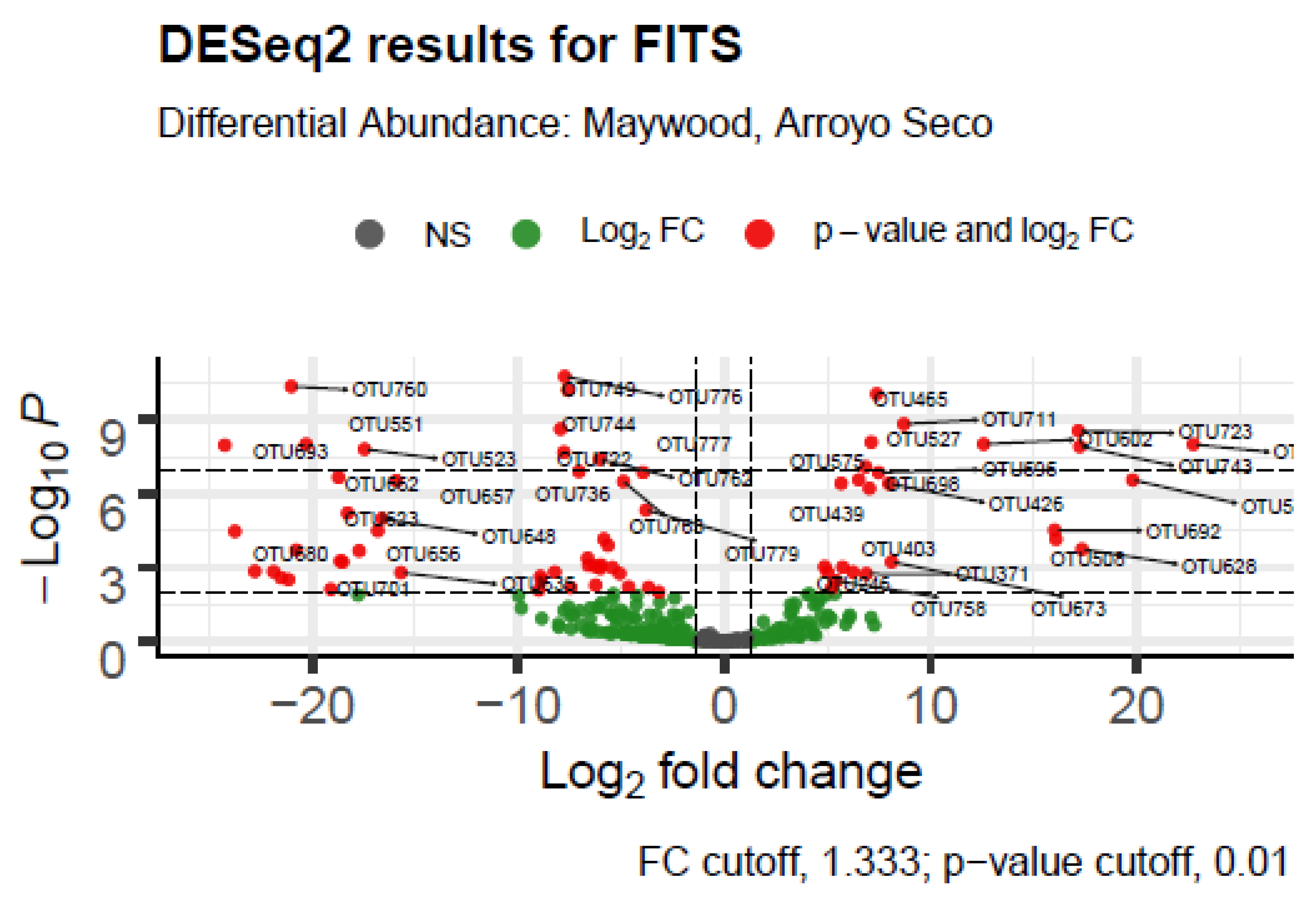
| FITS | LA River Site | Maywood, Arroyo Seco |
| L.A. RIVER | Branch Length NJ | Branch Length UPGMA | NJ vs. UPGMA | ||
|---|---|---|---|---|---|
| Marker | Mean | Variance | Mean | Variance | Tree Distance |
| FITS | 1657 | 5,419,114 | 1585 | 4,124,851 | 8195 |
| 16S | 620 | 460,349 | 609 | 417,224 | 2473 |
| 18S | 2018 | 5,534,355 | 1978 | 4,278,736 | 10,919 |
| COI | 2312 | 8,746,132 | 2114 | 6,010,691 | 9697 |
| 12S | 634 | 4,710,694 | 1585 | 4,124,851 | 12,130 |
| PITS | 1457 | 6,728,373 | 1351 | 4,241,554 | 8516 |
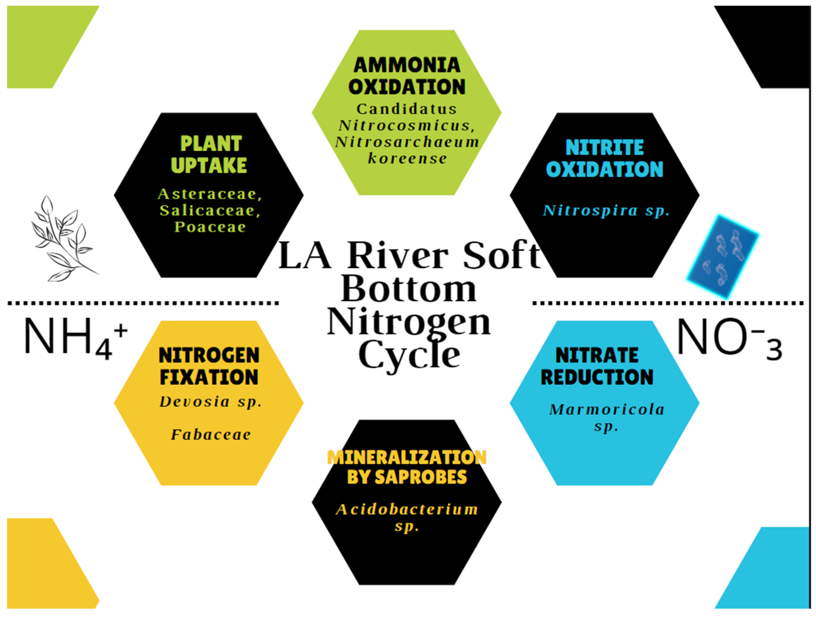
| Taxon | Log2 Fold Change | p-adj | Ecological or Metabolic Function and Pathogenicity |
|---|---|---|---|
| Prosthecobacter sp. | 22.09927 | 3.71 × 10⁻²³ | possible pathogen, anaerobic, tubulin-like genes, low nutrient environments |
| Dechloromonas sp. | 34.31956 | 1.53 × 10−41 | may oxidize benzene |
| Devosia sp. | −22.258 | 5.73 × 10⁻⁵ | nitrogen fixer |
| Bacillus sp. | −25.3115 | 1.67 × 10⁻⁵ | many beneficial species |
| Chromatiaceae (unclassified) | 23.78784 | 1.22 × 10⁻⁶ | purple sulfur bacteria, use sulfide to fix carbon and generate oxygen |
| Sandaracinobacter sp. | −30.519 | 0.009416 | metabolism of sulfide to cysteine (or from serine) |
| Chloroflexaceae (unclassified) | 25.68591 | 0.000938 | green non-sulfur bacteria, many heat-loving anoxygenic photoheterotrophs [38,39] |
| endosymbiont of Ridgeia piscesae | −22.3636 | 0.00014 | gammaproteobacterium, symbiont of a tubeworm |
| anaerobic bacterium MO-CFX2 Chloroflexi | −6.85917 | 4.08 × 10⁻⁶ | |
| Rhodocyclales (unclassified) | 17.1087 | 4.15 × 10⁻⁸ | nitrogen fixing or nitrogen reducing |
| Phormidium setchellianum | 33.82601 | 2.58 × 10⁻¹⁴ | potential cause of gastroenteritis, concentrates caused neuro- and hepato-toxicity in mice [40] |
| Cytophaga xylanolytica | 20.18264 | 0.000268 | xylan degrading, does well in sulfogenic and methanogenic environments, anaerobic and gliding |
| Synechococcus sp. | −23.4117 | 0.002659 | photolysis of sulfide or water, produces neurotoxins [41] |
| Scenedesmaceae (unclassified) | 11.0032 | 0.000123 | green algae, may degrade radioactive materials |
| Flavobacterium sp. | 8.245038 | 0.000199 | often associated with plant resistance to pathogens |
| Oscillatoriales cyanobacterium HF1 | 7.271474 | 0.005122 | cyanobacterium which may cause illness or death in humans and animals |
| Tetradesmus obliquus | 10.11933 | 0.001645 | produces valuable saturated and unsaturated esters, extract has anticancer and antimicrobial effects [42,43] |
| Microcystis sp. | 28.7773 | 1.03 × 10⁻⁷ | cyanobacterium which is toxic to humans [44] |
| Rhodocyclaceae bacterium enrichment culture clone Y62 | 28.91261 | 5.24 × 10⁻⁵ | nitrogen fixing or nitrogen reducing |
| Taxon | Log2 Fold Change | p-adj | Ecological or Metabolic Function and Pathogenicity |
|---|---|---|---|
| Oscillatoriales cyanobacterium YACCYB599 | −25.207183 | 3.06 × 10⁻²³ | cyanobacteria, which may cause illness or death in humans and animals |
| Chroococcus subviolaceus | −24.66764915 | 4.55 × 10⁻²³ | freshwater or high salinity environments, cyanobacteria which can survive with low O2 [45] |
| Haliea sp. | −24.50212313 | 4.55 × 10⁻²³ | marine gamma proteobacterium, which tolerates up to 12% salinity [46,47] |
| Halomonas sp. | 24.49667323 | 3.81 × 10⁻³¹ | chloride and saline tolerance |
| Marmoricola sp. | 24.12963073 | 1.43 × 10⁻²⁷ | denitrifying bacteria [48] |
| Alpha proteobacterium LS7-MT | 10.00393321 | 8.21 × 10−09 | methanol oxidizer, lives in high temperatures [49] |
| Nitrosarchaeum koreense | 9.188395232 | 2.37 × 10⁻¹⁸ | aerobic ammonia-oxidizing archaea [50] |
| Microcystaceae (unclassified) | −8.382519826 | 0.001244 | common eutrophic bloomer, toxin-producing cyanobacterium |
| Acidobacterium sp. SCGC AAA007-P13 | 7.849119335 | 3.12 × 10⁻⁷ | potential saprobe |
| Oscillatoriales cyanobacterium IRH12 | −7.732408042 | 4.32 × 10⁻⁸ | cyanobacterium, which may cause illness or death in humans and animals |
| Roseisolibacter agri | −7.389766623 | 0.000539 | grows in low oxygen environments [51] |
| Pleurocapsa concharum | −7.310779292 | 1.03 × 10⁻⁷ | ostracod-dependent cyanobacterium [52] |
| Devosia sp. | 7.242636088 | 5.51 × 10⁻⁷ | nitrogen-fixing bacteria |
| Nitrospira sp. enrichment culture clone LD3 | 6.970043209 | 0.001616 | nitrifying bacteria, nitrite-oxidizing bacteria |
| Gamma proteobacterium SCGC AAA007-P21 | 6.533527317 | 1.83 × 10⁻¹³ | uncultivated bacterioplankton |
| alpha proteobacterium Schreyahn_AOB_Aster_Kultur_5 | 6.503508981 | 0.001529 | cultured alphaproteobacterium |
| Chlamydomonadales (unclassified) | −6.479686479 | 0.000178 | green algae [53] |
| Chloronema giganteum | −6.382235759 | 0.000425 | photoautotrophic, anoxygenic green non-sulfur bacteria [54] |
| Chamaesiphon sp. | −6.230017507 | 0.002384 | widely distributed cyanobacterium [55] |
| Altererythrobacter sp. | 6.02052523 | 0.007591 | alkaline or salt tolerant aerobic phototroph, anoxygenic [56,57,58] |
| Mycobacteriaceae (unclassified) | 5.990283542 | 0.000524 | potential human and animal pathogens |
| Acidobacteriaceae (unclassified) | 5.737312813 | 2.78 × 10⁻⁶ | likely saprobe of plant organic matter |
| Candidatus Viridilinea mediisalina | −5.72085055 | 0.009826 | anaerobic phototroph, salt-tolerant and prefers alkaline environments [59] |
| Veillonellaceae bacterium 6–15 | −5.56037325 | 2.59 × 10⁻⁵ | bacterial vaginosis |
| Phormidium setchellianum | −5.548460876 | 0.000699 | cyanobacterium with possible antitumor agents, neuro and hepatotoxicity |
| Calothrix sp. UAM 374 | −5.531306605 | 0.003193 | cyanobacterium, which grows on plants and hard substrates [60] |
| Candidatus Nitrosocosmicus sp. | 5.344610141 | 0.0001 | aerobic ammonia-oxidizing archaea |
| Treponema stenostreptum | −5.019693824 | 0.003193 | syphilis relative |
| Leptolyngbyaceae (unclassified) | −4.952937198 | 0.001067 | thermophilic and potentially iron-loving cyanobacterium [61] |
| Holophagaceae (unclassified) | −4.934291389 | 0.000964 | anaerobic dweller of freshwater sediments [62] |
| Xanthomonadaceae bacterium | −4.711954167 | 0.002384 | potential phytopathogens |
| Leptolyngbya geysericola | −4.711366069 | 0.005914 | alkaline tolerant non-heteroctic cyanobacterium, produces calcite on microplastics [63] |
| Caldilineales bacterium | 4.50039412 | 4.71 × 10⁻⁶ | thermophilic and anaerobic [64] |
| Fusibacter sp. enrichment culture | −4.35065315 | 0.009823 | thiosulfate reducing, potentially halotolerant |
| Desulfomicrobium sp. | −4.16646108 | 0.002439 | oxidizes sulfide and arsenate in the presence of CO2 and acetate [65], reduces nitrate to ammonium [66] |
| Oscillochloridaceae (unclassified) | −3.874861377 | 0.005914 | anoxygenic phototrophic bacteria [38,67] |
| Pleurocapsales (unclassified) | −3.695598612 | 0.009826 | cyanobacterium from calcareous environments |
| Vicinamibacter silvestris | 3.602101991 | 0.002384 | polyphosphate accumulating organisms |
| Firmicutes (unclassified) | 2.378738101 | 0.004923 | high abundance in suburban rivers, negatively correlated with ammonia concentration |
| Stenotrophobacter terrae | 2.253024076 | 0.008829 | opportunistic pathogen |
| Vicinamibacteraceae (unclassified) | 2.126473277 | 0.00044 | degrades chitin [68] |
| Actinobacteria (unclassified) | 2.033767588 | 0.003193 | many denitrifying bacteria [69,70] |
| Botanical Name | Common Name | Category | Environment |
|---|---|---|---|
| Artemesia douglasiana | Douglas’ sagewort | Smaller shrubs and perennials | normal, moist, or saturated soils |
| Carex praegracilis | field sedge | Smaller shrubs and perennials | normal, moist, or saturated soils |
| Eleocharis macrostachya | common spikerush | Smaller shrubs and perennials | normal, moist, or saturated soils |
| Equisetum hyemale | horsetail | Smaller shrubs and perennials | normal, moist, or saturated soils |
| Juncus patens | common rush | Smaller shrubs and perennials | normal, moist, or saturated soils |
| Ribes aureum var. gracillimum | golden currant | Smaller shrubs and perennials | normal, moist, or saturated soils |
| Rosa californica | California wildrose | Smaller shrubs and perennials | normal, moist, or saturated soils |
| Verbena lasiostachys | vervain | Smaller shrubs and perennials | normal, moist, or saturated soils |
| Acer negundo | box elder | Larger shrubs and trees | normal, moist, or saturated soils |
| Acer rhombifolia | white alder | Larger shrubs and trees | normal, moist, or saturated soils |
| Baccharis salicifolia | mulefat | Larger shrubs and trees | normal, moist, or saturated soils |
| Juglans californica | black walnut | Larger shrubs and trees | normal, moist, or saturated soils |
| Platanus racemosa | California sycamore | Larger shrubs and trees | normal, moist, or saturated soils |
| Populus fremontii | Fremont cottonwood | Larger shrubs and trees | normal, moist, or saturated soils |
| Salix laevigata | red willow | Larger shrubs and trees | normal, moist, or saturated soils |
| Salix lasiolepis | arroyo willow | Larger shrubs and trees | normal, moist, or saturated soils |
| Sambucus mexicana | blue elderberry | Larger shrubs and trees | normal, moist, or saturated soils |
| Artemesia californica | California sagebrush | Smaller shrubs and perennials | riparian banks, not saturated |
| Asclepias fasiculata | narrow leaf milkweed | Smaller shrubs and perennials | riparian banks, not saturated |
| Encelia californica | bush sunflower | Smaller shrubs and perennials | riparian banks, not saturated |
| Eriogonum fasciculatum | California buckwheat | Smaller shrubs and perennials | riparian banks, not saturated |
| Lotus scoparius | deerweed | Smaller shrubs and perennials | riparian banks, not saturated |
| Salvia apiana | white sage | Smaller shrubs and perennials | riparian banks, not saturated |
| Salvia clevelandii | Cleveland sage | Smaller shrubs and perennials | riparian banks, not saturated |
| Salvia mellifera | black sage | Smaller shrubs and perennials | riparian banks, not saturated |
| Baccharis pilularis | coyote brush | Larger shrubs and trees | riparian banks, not saturated |
| Ceanothus spp. | California lilac | Larger shrubs and trees | riparian banks, not saturated |
| Heteromeles arbutifolia | toyon | Larger shrubs and trees | riparian banks, not saturated |
| Juglans californica | California walnut | Larger shrubs and trees | riparian banks, not saturated |
| Manzanita spp. | Larger shrubs and trees | riparian banks, not saturated | |
| Malosma laurina | laurel sumac | Larger shrubs and trees | riparian banks, not saturated |
| Platanus racemosa | California sycamore | Larger shrubs and trees | riparian banks, not saturated |
| Rhus integrifolia | lemonade berry | Larger shrubs and trees | riparian banks, not saturated |
| Sambucus mexicana | blue elderberry | Larger shrubs and trees | riparian banks, not saturated |
| Quercus agrifolia | coast live oak | Larger shrubs and trees | riparian banks, not saturated |
Disclaimer/Publisher’s Note: The statements, opinions and data contained in all publications are solely those of the individual author(s) and contributor(s) and not of MDPI and/or the editor(s). MDPI and/or the editor(s) disclaim responsibility for any injury to people or property resulting from any ideas, methods, instructions or products referred to in the content. |
© 2023 by the authors. Licensee MDPI, Basel, Switzerland. This article is an open access article distributed under the terms and conditions of the Creative Commons Attribution (CC BY) license (https://creativecommons.org/licenses/by/4.0/).
Share and Cite
Senn, S.; Bhattacharyya, S.; Presley, G.; Taylor, A.E.; Stanis, R.; Pangell, K.; Melendez, D.; Ford, J. The Community Structure of eDNA in the Los Angeles River Reveals an Altered Nitrogen Cycle at Impervious Sites. Diversity 2023, 15, 823. https://doi.org/10.3390/d15070823
Senn S, Bhattacharyya S, Presley G, Taylor AE, Stanis R, Pangell K, Melendez D, Ford J. The Community Structure of eDNA in the Los Angeles River Reveals an Altered Nitrogen Cycle at Impervious Sites. Diversity. 2023; 15(7):823. https://doi.org/10.3390/d15070823
Chicago/Turabian StyleSenn, Savanah, Sharmodeep Bhattacharyya, Gerald Presley, Anne E. Taylor, Rayne Stanis, Kelly Pangell, Daila Melendez, and Jillian Ford. 2023. "The Community Structure of eDNA in the Los Angeles River Reveals an Altered Nitrogen Cycle at Impervious Sites" Diversity 15, no. 7: 823. https://doi.org/10.3390/d15070823