
Large Remaining Forest Habitat Patches Help Preserve Wild Bee Diversity in Cultivated Blueberry Bush
by

Sergio Vega
1,†,
Héctor Vázquez-Rivera
1,†,
Étienne Normandin
2,
Valérie Fournier
3 and
Jean-Philippe Lessard
1,* 1
Department of Biology, Concordia University, Montreal, QC H3G 1M8, Canada
2
Institut de Recherche en Biologie Végétale, Université de Montréal, Montréal, QC H1X 2B2, Canada
3
Centre de Recherche et d’Innovation sur les Végétaux, Université Laval, Québec, QC G1V 0A6, Canada
*
Author to whom correspondence should be addressed.
†
These authors contributed equally to this work.
Diversity 2023, 15(3), 405; https://doi.org/10.3390/d15030405
Submission received: 6 January 2023
/
Revised: 6 March 2023
/
Accepted: 6 March 2023
/
Published: 10 March 2023
(This article belongs to the Special Issue Diversity of Terrestrial Invertebrate Communities)
Abstract
:Global declines in wild and managed bee populations represent a major concern for the agricultural industry. Such declines result, in part, from the loss of natural and semi-natural habitats in and around agricultural ecosystems. However, remaining forest patches in heavily modified landscapes represent nesting habitats that may be crucial to preserving wild bees and their services. Because wild bees are the main pollinators of fruit crops, preserving potential nesting habitats might be particularly important for the crops’ yield and profitability. Here, we assessed whether the abundance and richness of visiting wild bees in blueberry crops relates to the amount of surrounding forest cover and if so, whether those relationships varied with spatial scale. Specifically, we sampled wild bee communities in 18 blueberry fields during the blooming period in Montérégie, Quebec, Canada, where sampling consisted of pan trap triplets and direct observation of flower visitors on blueberry bushes. Then, we quantified the proportion of forest in radii of 0.5 km, 1 km, and 2 km around each field. Wild bee abundance was positively related to the proportion of forest habitat surrounding the crop field, but the relationship for wild bee richness was less clear. Moreover, these relationships were strongest at 1 and 2 km radii of measured land cover. Overall, pollinator diversity was highest when at least 30% of the surrounding landscape consisted of forest patches, representing a total area of at least 1 km2. Our results suggest that preserving large habitat patches in agricultural landscapes can help prevent further decline in wild bee diversity while maximizing pollination services to fruit crops.
1. Introduction
Agricultural ecosystems rely on both domesticated and wild bees for pollination [1]. Although managed honey bees (Apis mellifera Linnaeus) pollinate many crops, wild bees enhance pollination and yields even in the presence of honey bees [2,3,4,5]. Indeed, bee pollination services contribute to the productivity of >75% of the world’s crop species [6,7]. Therefore, wild bees can substitute for the services that managed pollinators provide, replacing them either fully or partially [8], while often being more efficient [9]. Wild bees can also enhance productivity in plants that self-pollinate, and for which managed pollination is rare [8]. Clearly, as managed honey bees around the world face serious threats from diseases, pesticides, and other causes, wild bees represent an important insurance policy for agro-ecosystems [5].
Natural forest remnants in intensive agricultural landscapes can provide safe haven for insect pollinators [2,4]. Natural and semi-natural habitats around agricultural fields provide food and nesting resources that contribute to the long-term persistence of wild bee populations [8]. The presence of forest cover surrounding crop systems can therefore exert a positive influence on wild bee diversity and the services they provide [3,4,8]. Nevertheless, explicit quantification of the amount of natural habitat necessary to maximize the diversity of visiting crops, as well as the spatial scale at which natural habitat availability has an influence, is crucial to inform landscape management.
Wild bees are an essential but underrated player in the production of blueberries in North America. In Canada, highbush blueberries (Vaccinium corymbosum L.) are the largest fruit commodity, representing an average market value of USD 220 M between 2015 and 2020 [10]. Despite producers relying heavily on honey bees for pollination, wild bees are the most efficient pollinators of highbush blueberry [11,12,13,14]. This likely results from wild bees’ co-evolutionary history with highbush blueberries [14,15], which allows bees to deposit more pollen grains to the stigma per flower visit [13,14,15]. Furthermore, northern wild bees can forage during the cool, wet spring weather [13,15] typical of the highbush blueberry blooming season at northern latitudes (May–June). Nevertheless, it remains unclear how much natural habitat is required to sustain wild bee diversity and associated pollination services in blueberry fields.
Here, we assess whether the wild bee community observed in blueberry bushes during blooming relates to the adjacent natural cover. We predicted that the abundance and richness of wild bees in blueberry fields increase with the proportion of surrounding forest habitat. Furthermore, we investigated the spatial extent at which these relationships are strongest.
2. Materials and Methods
2.1. Study Area
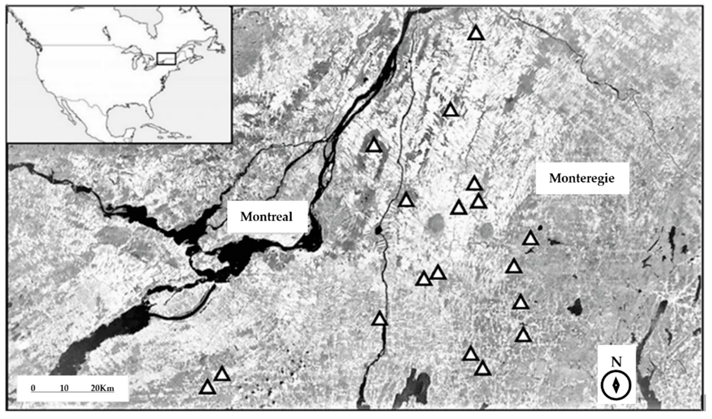
The study was conducted in 18 highbush blueberry (Vaccinium corymbosum L.) fields (sampling sites) in Montérégie, Quebec, Canada (Figure 1). Fields included Patriot, Blueray, Burkley, and Bluecrop varieties, and had a surface area of at least 0.5 ha (Supplementary Material; Table S1). The sites were separated from one another by an average minimum distance of ~10 km (min. ~5 km and max. min. ~24 km). The study region included crops of corn, soybean, and hay, as well as smaller quantities of apple orchards, vineyards, and small fruit plantations, such as strawberry and blueberry fields [16]. Regarding natural land cover, the landscape consists of fragmented coniferous and deciduous forest patches, and semi-natural areas, such as grasslands, meadows, hedgerows, marshlands, pastures, and abandoned fields [17].
2.2. Wild Bee Sampling
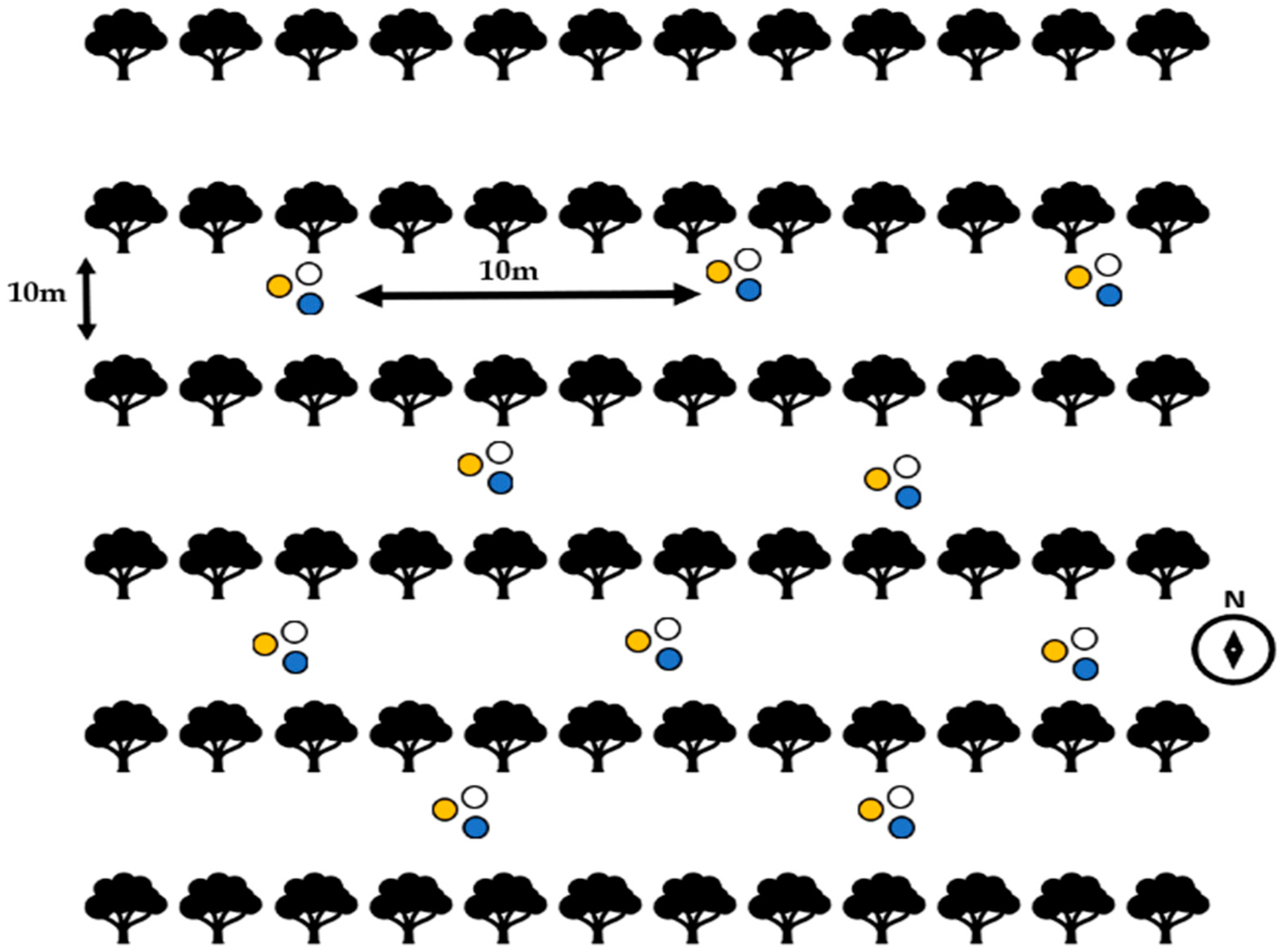
We performed two visiting rounds to each sampling field throughout the blooming season, from 23 May 2017 to 9 June 2017. At each field, we deployed 10 sampling stations in a grid, with at least 10 m separating each station (Figure 2). We established a standardized quadrant distribution that would sample as much terrain as possible without exceeding the size of smaller crops. This distribution began at the western middle point of each field and progressed towards the east. To have a better representation of the bee community present in each field, we implemented two complementary sampling techniques: (i) visuals/observations of visits on blueberry flowers and (ii) pan trap triplets deployed on the ground.
The visual technique consisted of recording bees that entered the flower legitimately and apparently contacted the stigma [18]. A visual survey was performed on blooming sections of shrubs located in front of the pan trap triplets at standpoint view for 5 min at each sampling station, meaning 50 min observation per field per visiting round, for a total of 1800 min. We identified visiting bees on the fly by using a morphotype guide that included photos of bees present at blueberry bloom in the same region, in the previous year (i.e., 2016). Honey bees (Apis mellifera L.) and bumble bees (Bombus spp.) were identified to species on the fly. Morphotypes that were not in the photo guide, but observed foraging on blueberry flowers, were net captured. Because these crops were commercial, growers were worried about the potential negative impact of swinging a net over the shrubs during blooming season. Consequently, we only swung the net when deemed necessary in order to circumvent this issue. Collected specimens were later identified. The number of wild bees collected with this technique was described as flower visits while the variety of morphotypes was described as visiting-richness. The honey bee visits were counted but the data were not used in any statistical analysis.
Pan trapping is a standard method for sampling bees that reduces observer bias, although it may perform poorly for some taxa [17,19]. A pan trap triplet, as used in this study, was composed of three 500 mL plastic containers. Each container was painted with either fluorescent yellow or blue Krylon® paint on the interior surface or left unpainted as opaque white. Each container was filled with 250 mL of water and 1 drop of non-fragrant liquid soap (detergent) to break surface tension [9,19]. At each sampling station, one pan trap triplet was installed (Figure 2). For the first visit, the traps were left to collect data for 24 h, while for the second round, they were kept for 48 h. As a result, 10 stations per site yielded a total of 30 sampling containers. After each sampling period, specimens were stored in 70% ethanol until pinned. The number of wild bees quantified with this technique was described as trapped abundance while the variety of morphotypes was described as trapped richness. To describe the expected general pattern, that is without distinguishing between data from the visual technique and the pan traps technique, the number of wild bees was referred to as abundance whereas the variety of morphotypes as richness.
Bees in the laboratory were identified using taxonomic classification books based on dichotomous keys such as the “Bee Genera of Eastern Canada” [20], “Bees of the World” [21], and “Bumble Bees of North America” [22]. Identification was validated by personnel from the Centre de Recherche et d’Innovation sur les Végétaux at Université Laval in Quebec City and the Entomological Collection Ouellet-Robert (QMOR) at Université de Montréal. Specimens not identified at the species level were assigned a morphotype.
2.3. Environmental Variables
Because daily fluctuations in temperature can affect the level of bee activity in blueberry fields [15], visual sampling took place between 10:00 h and 17:00 h on sunny to partially sunny days. Air temperature data were obtained from weather stations records available on Canada’s environmental and natural resources website (Government of Canada, 2017). The average minimum distance between a given sampling field and the closest weather station to that field was 8.8 km (min ~1 km; max. min ~17.8 km). Leaf temperature in the sampling sites was registered to have a more accurate indicator of how environmental temperature might affect bees’ presence. It was registered with a digital infrared thermometer Earme model GM320, within a standardized distance of 30 cm from blueberry leaves at every sampling station at the time of performing visual samplings.
2.4. Surrounding Land Cover
Five land cover types surrounding blueberry fields were identified: (1) agricultural [23], (2) forest/woodland, (3) urban, (4) water, and (5) abandoned/semi-natural areas [24], described as the remaining area in the landscape, which include spiny shrub vegetation, pasture fields, hydric herbaceous, and shrub vegetation [24]. Urban and water bodies categories were unrepresented (Supplementary Figure S1) and including them in the analysis did not add any information (data not presented here). Thus, they were not considered. Agricultural cover had the opposite effect of forest; because our objective was to study the effect of natural/seminatural cover, we also discarded agriculture from the analysis. All data were in vector format as shapefiles [25].
We extracted land cover types within radii of 500 m, 1000 m, and 2000 m (i.e., different spatial extents or scales) from the sampling sites using the buffer and clip tools in ArcGIS [25]. Then, we determined the proportional area that each landcover type occupied within the different radii. Sampling land cover at different scales has been used to characterize the surrounding landscape of focal sites in studies of crop pollination by native bees, and it has been shown that across scales, varying from 600 m to 4200 m radius, the coefficient of determination (R2) for the positive relationship between bee flower visit and the proportion of nearby natural land cover, reaches a plateau at ca. 2000 m radius [26]. Therefore, we were interested in testing our prediction at the 2000 m radius. However, we sampled at the three scales to determine if the relationship between bee community structure and natural land cover would hold across those scales.
2.5. Statistical Analysis
The statistical analyses for the visual data and for the pan traps data were carried out separately for three reasons. First, the sampling protocol and effort differ between sampling techniques; second, the visual data allows making a more plausible connection between the wild bee community and the pollination service bees provide to blueberry crops; third, the pan traps data in parallel with the visual data, allows visualizing that wild bee conservation in agricultural areas is possible if, at least, a given proportion of natural cover is maintained in the landscape. We predicted that flower visits (the number of individuals) and visiting-richness (the number of morphotypes), as well as trapped abundance and trapped richness, of wild bees, observed in blueberry fields, were positively related to the proportion of available forest habitat surrounding blueberry fields. To evaluate this prediction, we first fitted four simple regression models separately, one for each case: flower visits, visiting-richness, trapped abundance, and trapped richness, as a function of the proportion of forest land cover.
We then fitted multiple regressions models to evaluate potentially important factors (i.e., confounding factors) whose omission might result in biased estimations of the forest land cover effect on the wild bee communities. Four factors were initially considered: (i) shrub density (number of blueberry plants per hectare), (ii) air temperature, (iii) leaf temperature, and iv) abandoned fields cover. However, air temperature and leaf temperature were collinear (r = 0.52, p = 0.027). Because collinear predictors can impact parameter estimates and potentially reduce the predictive accuracy of models, we retained only one of the collinear factors (see below). Each factor we modeled was retained a priori according to the rationales described below. Shrub density was considered because a higher density may represent more resources and result in higher bee abundance and richness. Leaf temperature was taken into account as ectothermic organisms (such as bees) alter their activity in response to environmental temperatures. The temperature of the sampling day could potentially affect the number of bees present in the field of focus, making it an important factor to consider. Abandoned fields were included because they are considered semi-natural habitats and have been suggested to support wild bee communities and therefore promote pollination services in agricultural fields [4]. To assess a given confounding factor while accounting for the effect of forest land cover, we added that given factor as a covariate to the initial model built on forest land cover only. We also assessed each confounding factor independently, i.e., without accounting for the effect of forest land cover (details below).
We used generalized linear models (GLMs) because our response variables were point count data, and count data often present Poisson or Negative Binomial distributions properties [27]. As there were five sites out of 18 with zero values for trapped wild bee abundance and richness, we also used Hurdle models to investigate whether the zero and positive values of the pan traps data were explained by the independent variables [28,29].
For each variable that we modeled, we reported the incidence rate ratio (IRR) estimate and its significance based on 95% confidence intervals. We did not consider the effects that multiple confounding factors at once may have on the forest land cover model, since our focus was to determine how a single confounding factor might modify the effect of forest. Furthermore, including several (>2) terms in the model might result in overfitting given our sample size (n = 18), causing model parameters to be heavily affected by the noise, and therefore increase the error in the model’s predictions [30].
To assess the strength of evidence of the effect of each independent variable on the dependent variables, in a uni- or bi-variate model, we fitted generalized linear models (GLMs), followed by estimates of the Akaike information criteria for small samples (AICc) [31,32]. We further reported the Nagelkerke’s likelihood ratio adjusted pseudo-R2 value for each model as the goodness of fit measure. For GLMs, Nagelkerke’s R2 is equivalent to the adjusted-R2 of multiple OLS regressions [33,34]. All GLMs were performed after testing for overdispersion in the conditional distribution of the outcome variables. We also tested for spatial autocorrelation in the models’ residuals to evaluate data independence. In all cases, no spatial autocorrelation was detected (–0.14 < Moran I < 0.09; p > 0.09).
Finally, to evaluate the spatial extend-dependency of the results, we report the observed relationship between independent and dependent variables for each studied scale (500 m, 1000 m, and 2000 m radius). Poisson regressions were fitted with the function glm from the package stats v3.4.3 [35], negative binomial regressions with the function glm.nb from the package MASS [36] and Hurdle models with the function Hurdle from the package pscl v1.5.5 [29]. Spatial autocorrelation was tested with the function testSpatialAutocorrelation from the package DHARMa [37]. All the analyses were performed in R version 3.6.3 [35].
3. Results
We sampled 39 different wild bee morphotypes, corresponding to 12 genera (Table 1). A total of 659 bees were observed visiting flowers legitimately, i.e., through visual observation, whereas 69 bees were captured with pan traps. Admittedly, the low number of bees caught with pan traps might cast doubt on our ability to accurately estimate community structure with this technique. However, wild bees seem to be caught in low numbers in berry crops [38] and orchards [39]. Nevertheless, we proceeded to test our prediction with the data collected for that purpose.
Based on the visual technique, Bombus spp. and Andrena spp. dominated the flower visits, with 66.3% and 23.07% respectively. Bombus spp. was represented by five distinguishable species (Table 1): B. impatiens was the most abundant species at most sites, comprising nearly 85.5% of all sampled bumble bees; B. ternarius followed in importance with approximately 13%; B. bimaculatus, B. terricola, and B. perplexus showed less than 1% of the total individuals observed.
In the pan traps (Table 2), Lasioglosum spp. and Andrena spp. were the most abundant bees, representing 46.38% and 20.29% of trapped abundance, respectively. Colletes spp. and Ceratina spp. were among the least represented pollinators, with less than 3% of the trapped abundance. Bombus spp. was not captured with this technique.
3.1. Surrounding Land Cover
The proportion of forest land cover (Supplementary Figure S1), mainly deciduous forests, increased from 18% to 27% with increasing spatial extent, but the proportion of abandoned fields, mostly scrublands, meadows, and pastures, decreased from 40% to 31%. Agricultural habitats, water bodies, and urban structures remained unchanged across scales, representing respectively 39, 2.5, and <1% of land cover.
3.2. The Influence of Natural Habitat
We predicted that wild bee abundance and richness would be positively related to the proportion of available forest habitat surrounding blueberry fields. Recall that we show the results from the visual and pan traps techniques separately.
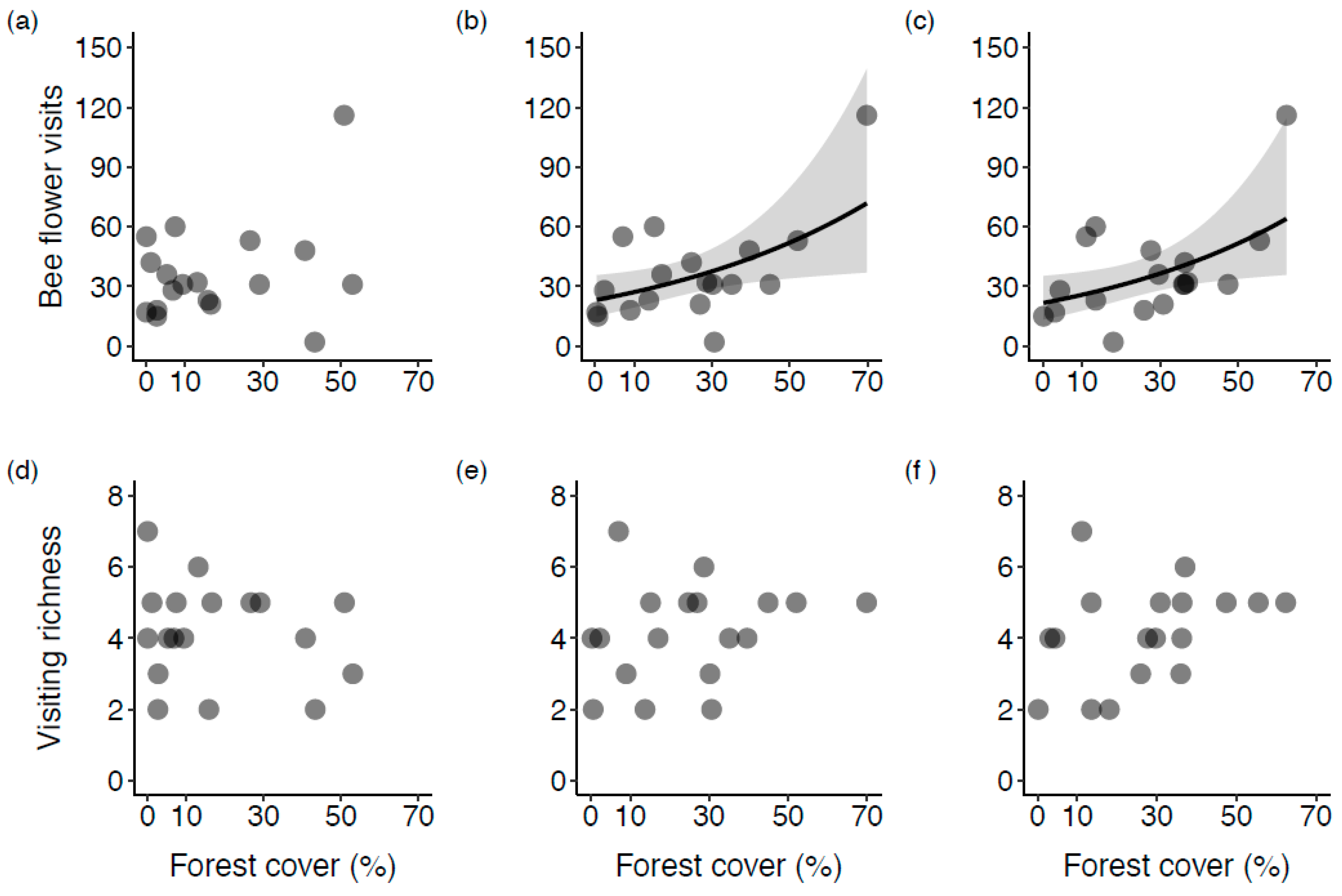
Based on the GLMs for the observational data (Table 3), we found that forest land cover alone had a statistically significant and positive effect on bee flower visits at the 1000 and 2000 m radii (IRR > 1; Figure 3b,c), but not at the 500 m radius (Figure 3a). When potentially confounding factors were added to the models on bee flower visits, i.e., fitting bivariate models, the effect of forest cover remained positive and statistically significant. However, the bivariate model was not significant when leaf surface temperature was included as a covariate in the forest model. Leaf temperature, after controlling for forest effect, showed no effect either (Table 3). Overall, the confounding factors had no effect on wild bee flower visits. For visiting-richness, we did not find a correlation between forest land cover, confounding factors, and the number of morphotypes visiting blueberry flowers at the three different scales (Figure 3d–f, Table 3). This could be due to limited visual observations or a small sample size.
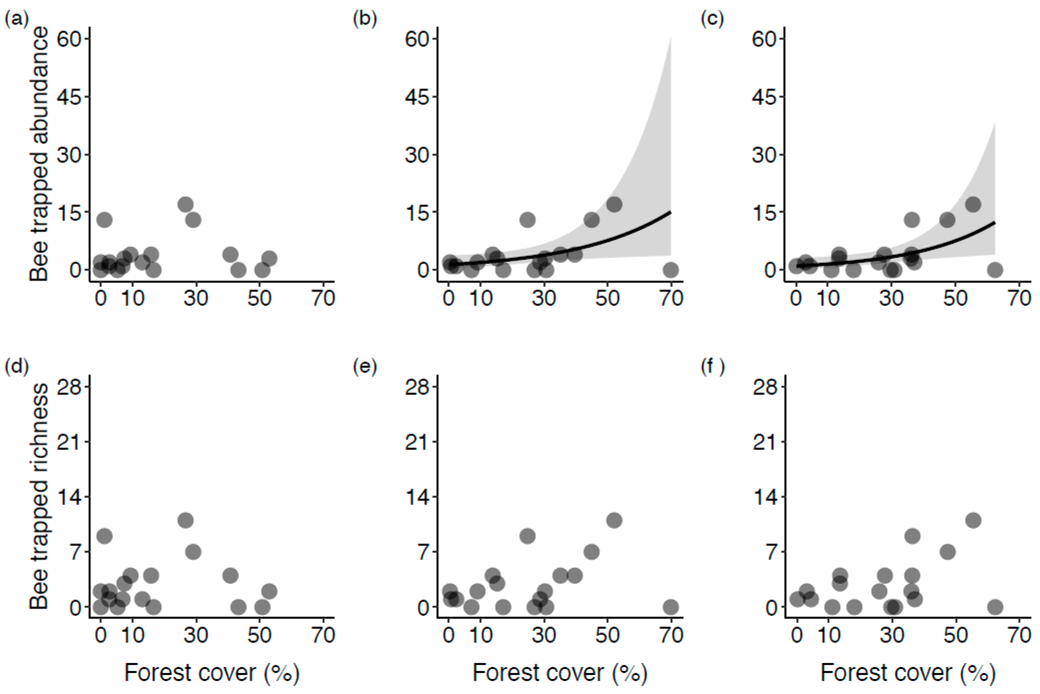
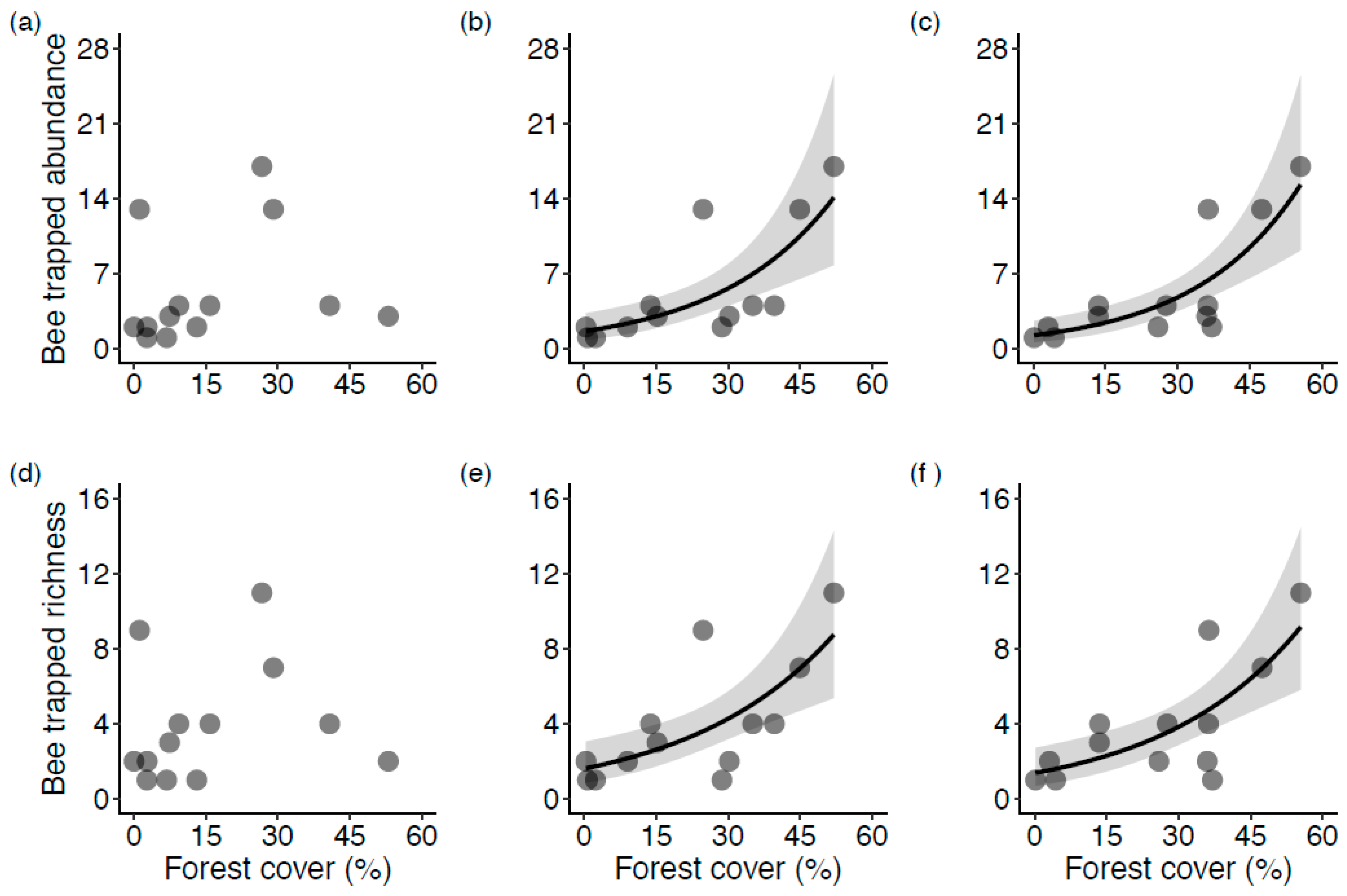
The GLMs for the pan trap data (Table 4) showed that, at the 2000 m radius, the effect of forest land cover on the abundance of trapped wild bees was positive and statistically significant in both univariate (Figure 4c) and bivariate models (IRR > 1). In the bivariate models, the confounding factors showed no effect at this scale. At the 1000 m radius, forest alone (Figure 4b) or modeled together with shrub density showed a positive and significant effect on trapped abundance, but not when it was modeled together with abandoned fields, which showed a positive and significant effect (Table 4). At the 500 m radius, forest alone (Figure 4a) or modeled together with a confounding factor (Table 4) did not affect bee-trapped abundance. Instead, abandoned fields showed a positive and significant effect on trapped abundance after accounting for forest land cover. Regarding wild bee richness from pan traps (Table 4), forest land cover modeled alone (Figure 4d–f) or together with a confounding factor, showed no effect on the number of morphotypes captured in the blueberry fields; this was consistent across the three different scales. In contrast, after accounting for forest land cover, abandoned fields showed a positive and significant effect on the wild bee trapped richness at the 1000 m and 500 m radii (Table 4).
The Zero-Hurdle models (due to the number of sites with no bee data) showed that none of the independent variables determined a zero or a positive value of wild bee trapped abundance (Table S5) or trapped richness (Table S6) in a given blueberry field. However, the truncated or Count-Hurdle models revealed that forest land cover, but not the confounding variables, had a statistically significant effect on the positive values of trapped abundance (Figure 5b,c; Table S5) and trapped richness (Figure 5e,f; Table S6). This result was consistent at the 2000 m and 1000 m radii. Neither forest land cover nor the confounding variables showed any effect on wild bee trapped abundance or richness at the 500 m radius (Figure 5a,d).
In terms of goodness of fit (Nagelkerke’s R2) and the strength of evidence (AICc), the GLM models based on the visual technique data (Table S2) indicate that forest land cover is a predictor stronger than the confounding factors, of wild bee flower visits at the 2000 m and 1000 m scales. At the 500 m scale, however, leaf temperature was the most important predictor of flower visits, whereas forest land cover and abandoned fields came in second and third place, respectively. For the visiting richness, the result shows that plant density, forest cover, and abandoned fields were the first, second and third most important predictors respectively; this was consistent across the three scales (Table S2). The models based on pan traps data (Table S3) show that forest is the strongest predictor of wild bee trapped abundance and trapped richness observed in the blueberry fields (not visiting flowers) only at the 2000 m scale; at the 1000 m and 500 m scale, forest’s importance falls much below the importance of abandoned fields, which became the main predictor (Table S3). Regarding Count-Hurdle models for the pan traps data (Table S4), the results showed that forest land cover was the most important factor in explaining the spatial variation of both trapped abundance and trapped richness in the blueberry fields, at the 2000 m and 1000 m scales (Figure 5b,c,e,f). Abandoned fields and plant density were among the second most important predictors of trapped abundance and richness at those scales (Table S4). At 500 m radius, abandoned fields and leaf temperature were the first and second most important variables, respectively, in accounting for the spatial variations of abundance and richness. Forest land cover was the third most important predictor of wild bee trapped abundance at this scale, but not of trapped richness (Table S4).
4. Discussion
The results were consistent with our predictions that higher values of wild bee abundance and richness would be associated with a larger proportion of forested land cover. This relationship at 2000 m and 1000 m scales is in accordance with earlier studies suggesting that the presence of bees in crops and thus pollination services rely on natural areas adjacent to farmlands [18,26,40,41]. At 500 m, however, this relationship was not observed. Our results indicate that forest land cover near blueberry fields can help sustain the abundance, richness, and flower visitation of wild bees in these crops.
4.1. The Effect of Forest Proportion on Wild Bee Diversity in Blueberry Fields
Blueberry fields in areas with a larger proportion of remaining forest had higher flower visits and higher number of wild bee species Figure 3b,c, Figure 4b,c, and Figure 5b–d,f), which is consistent with previous similar studies. For example, Watson et al. [41] found that wild bee abundance was positively related to the proportion of forest land cover surrounding sampled apple orchards. Similarly, Benjamin et al. [18] showed that wild bee abundance decreases with agricultural land cover within 300 m and 1500 m radii. However, a study also conducted in fruit crops of southern Quebec concluded that fruit crops diversity in the region as well as the proximity to suburban areas had a positive effect on wild bee diversity (richness and abundance) at the landscape level (380–2000 m radii) [42]. As such, our study somewhat contradicts these results, but one has to consider that Martins et al. [42] also included apple orchards and raspberry fields in their study, which differ from the specific wild bee species composition from blueberry field. Other factors to consider that potentially can result in differences in abundance and richness of pollinators between studies are the differences in sampling effort, the sampling techniques, and the sampled fields’ surroundings.
The higher numbers of flower visits and bees associated with a higher proportion of forest cover observed in this study are relevant from the pollination service perspective [26,40] and therefore to blueberry production [3]. Evidence shows that different types of crop production increase with the frequency of wild bee flower visits [43,44,45]. In blueberry fields, wild bee pollination efficiency is known to be two to four times higher than that of honey bees [11,13], but see [46]. In this study, the lack of data on yield from a larger number of farms prevented us from assessing fruit set. Nevertheless, the evidence indicates that farmers may be able to increase the production of marketable fruits by increasing natural area near their blueberry fields.
Although the proportion of surrounding abandoned fields did not influence the number of bee flower visits and abundance in pan traps, it had a strong and positive influence on bee richness, which aligns with a previous study in the same region. Martins et al. [42] studied local- and landscape-level drivers of bee diversity and argued that wild bee abundance and richness observed in croplands (including apple orchards, raspberry and blueberry fields), respond positively to hedgerows and meadows habitats because they provide nesting and foraging resources for wild bee communities observed in those crops. Hedgerows and meadows habitats are included in the abandoned fields category in the present study.
4.2. The Role of Bumble Bees and Incidental Visitors
Our results indicate that bumble bees in southern Quebec are the most active native pollinators on highbush blueberry flowers during blooming (Table 1). Indeed, as previously stated, the genus Bombus spp., with five species, accounted for 66.3% of the observed wild bee abundance. Estimates for a geographic region near to our study area, show that Bombus spp. provide ~75% of the pollination in blueberry fields nested in landscapes dominated by woodland and ~5% in commercial fields [15]. Similarly, Bombus spp. would pollinate up to 6.5 flowers in the same lapse of time that honeybees would pollinate one flower [13]. Arguably, Bombus spp. is the most efficient pollinator in these agroecosystems due to its co-evolutionary history with Vaccinium spp. and its sonification pollination behaviour [15,47,48]. Conversely, bees caught in the pan traps seemed to be incidental visitors that had little part in the highbush blueberry crops’ pollination. However, andrenid bees and halictid bees are among the pollinators observed to perform high rates of legitimate flower visits to blueberry flowers [15].
Although B. impatiens represented 85.5% of all sampled bumble bees, its presence is unlikely to be related to managed colonies; growers participating in this study reported no use of commercial B. impatiens to provide sufficient pollination, but its use should not be disregarded. A study over 150 years of Bombus records in northeastern US, indicates that 11 out of 16 species show declining trends while seven species have increased, with B. impatiens being the most successful wild bee [49]. Plausible reasons for population shifts in wild bees may include but are not limited to landscape changes, fragmentation of optimal bee habitat, climate change, pesticide impact, ecological displacement by competition, and the use of managed colonies of species such as B. impatiens [14,49,50].
4.3. Assessing the Effective Spatial Scale of Natural Habitat Preservation
The spatial extent to which preserving natural habitat patches is meaningful remains poorly explored. Here, wild bee abundance, richness, and rates of visitations are positively associated with the amount of forest habitats available in a 1- or 2-km radius around blueberry fields. However, there is no such relationship when considering forest habitat cover in a 0.5-km radius. These results are consistent with the fact that some wild bees are known to forage in a 2-km radius from their nest, while others can go as far as 11 km or more [44,45,50,51,52]. Further, ground-nesting bee abundance has been reported to increase in sites with higher forest cover within 2 km [53], and croplands farther than 2 km from natural areas show a decrease in visitation rate [3]. Together, these results might reflect the ability of wild bees to travel long distances, but also that the sampling distance of 500 m, at least in this study, did not capture the forested source where the bees come from.
4.4. Landscape Management and Conservation Perspectives
Our research can be used as a guide to determine how much natural habitat should be preserved around highbush blueberry crops. It is recommended that the distance considered when assessing the availability of natural habitat should be no less than 500 m, but preferably stay between 1 and 2 km. Approximately 30% of the area around farms should be dedicated to forest habitats, as this is the minimum amount of cover that should be provided. Moreover, to guarantee optimal pollination of neighboring crops, it is recommended that forest remnants should have a minimum area of 1 km2. Despite the rarity of large forest patches in the study region and in other intensively farmed areas globally, there are still various measures that could be taken to ensure these patches can provide pollinator habitats. Monitoring patch sizes in agricultural landscapes and establishing buffer zones around forest patches with native trees and shrubs are two possible ways to protect them from land use changes. Additionally, creating pollinator-friendly habitat corridors to connect larger remnant patches and educating farmers and landowners about the importance of preserving and increasing pollinator habitats are important actions that should be taken.
Developing landscape management strategies to maintain wild bee diversity in agricultural ecosystems also requires considering both natural and semi-natural habitat types. Our results suggest that abandoned fields can be an important factor for wild bee abundance and richness at the 500 m scale (Table 3). Abandoned fields, being considered as a semi-natural land cover, positively influence wild bee diversity, perhaps because they provide alternative nesting habitats, or harbor a high diversity of flowers. We suggest that this might be particularly true when forest habitats are not well represented in the landscape. Therefore, strategic landscape management that favors semi-natural habitats as well could benefit wild bee diversity in agroecosystem settings. Clearly, wild bee conservation strategies should consider the availability of natural and semi-natural habitat patches at multiple spatial scales.
Supplementary Materials
The following supporting information can be downloaded at: https://www.mdpi.com/article/10.3390/d15030405/s1, Figure S1. Boxplots showing the proportional area of different land cover types sampled within (a) 500 m, (b) 1000 m, and (c) 2000 m radii in the landscape surrounding highbush blueberry fields; Table S1: Geographic coordinates, area, and highbush shrub density; Table S2: GLM based on visual technique data; Table S3: GLM based on pan trap data; Table S4: Count-Hurdle models for pan traps data; Table S5: Zero-Hurdle models for wild bee trapped abundance; Table S6: Zero-Hurdle models for wild bee trapped richness.
Author Contributions
Conceptualization, S.V. and J.-P.L.; methodology, S.V., H.V.-R. and J.-P.L.; formal analysis, H.V.-R.; investigation, S.V.; data curation, S.V. and H.V.-R.; writing—original draft preparation, S.V., H.V.-R. and J.-P.L.; writing—review and editing, S.V., H.V.-R. and J.-P.L.; visualization, S.V. and H.V.-R.; supervision, É.N., V.F. and J.-P.L.; funding acquisition, S.V. and J.-P.L. All authors have read and agreed to the published version of the manuscript.
Funding
This research was funded by Agronova, Beebio, and MITACS Accelerate Entrepreneur ref. IT06662. HVR received postdoctoral funding from CONACyT, Mexico: 100397-454840.
Data Availability Statement
All raw data are available on request (https://zenodo.org/). No novel code or computer software were used to generate results or analyses.
Acknowledgments
We thank the blueberry growers that allowed us to access their fields. Special thanks to Benoit Girard from Agronova for supporting the project. We are grateful to Amélie Gervais from the Centre de Recherche et d’Innovation sur les Végétaux (CRIV) at Laval University for helping with bee taxonomy; Stephanie Leduc, Carly McGregor, and William Doyon for their support in the field; and Frederic McCune for constructive comments on an advanced version of the manuscript.
Conflicts of Interest
The funders had no role in the design of the study; in the collection, analyses, or interpretation of data; in the writing of the manuscript; or in the decision to publish the results.
References
- Potts, S.G.; Biesmeijer, J.C.; Kremen, C.; Neumann, P.; Schweiger, O.; Kunin, W.E. Global Pollinator Declines: Trends, Impacts and Drivers. Trends Ecol. Evol. 2010, 25, 345–353. [Google Scholar] [CrossRef]
- Kennedy, C.M.; Lonsdorf, E.; Neel, M.C.; Williams, N.M.; Ricketts, T.H.; Winfree, R.; Bommarco, R.; Brittain, C.; Burley, A.L.; Cariveau, D.; et al. A Global Quantitative Synthesis of Local and Landscape Effects on Wild Bee Pollinators in Agroecosystems. Ecol. Lett. 2013, 16, 584–599. [Google Scholar] [CrossRef]
- Garibaldi, L.A.; Steffan-Dewenter, I.; Kremen, C.; Morales, J.M.; Bommarco, R.; Cunningham, S.A.; Carvalheiro, L.G.; Chacoff, N.P.; Dudenhöffer, J.H.; Greenleaf, S.S.; et al. Stability of Pollination Services Decreases with Isolation from Natural Areas despite Honey Bee Visits. Ecol. Lett. 2011, 14, 1062–1072. [Google Scholar] [CrossRef]
- Hevia, V.; Bosch, J.; Azcárate, F.M.; Fernández, E.; Rodrigo, A.; Barril-Graells, H.; González, J.A. Bee Diversity and Abundance in a Livestock Drove Road and Its Impact on Pollination and Seed Set in Adjacent Sunflower Fields. Agric. Ecosyst. Environ. 2016, 232, 336–344. [Google Scholar] [CrossRef]
- Winfree, R.; Williams, N.M.; Dushoff, J.; Kremen, C. Native Bees Provide Insurance against Ongoing Honey Bee Losses. Ecol. Lett. 2007, 10, 1105–1113. [Google Scholar] [CrossRef]
- Hanley, N.; Breeze, T.D.; Ellis, C.; Goulson, D. Measuring the Economic Value of Pollination Services: Principles, Evidence and Knowledge Gaps. Ecosyst. Serv. 2015, 14, 124–132. [Google Scholar] [CrossRef] [Green Version]
- Klein, A.-M.; Vaissiere, B.E.; Cane, J.H.; Steffan-Dewenter, I.; Cunningham, S.A.; Kremen, C.; Tscharntke, T. Importance of Pollinators in Changing Landscapes for World Crops. Proc. R. Soc. B Biol. Sci. 2007, 274, 303–313. [Google Scholar] [CrossRef] [Green Version]
- Williams, N.M.; Kremen, C. Resource Distributions among Habitats Determine Solitary Bee Offspring Production in a Mosaic Landscape. Ecol. Appl. 2007, 17, 910–921. [Google Scholar] [CrossRef]
- Moisan-Deserres, J.; Girard, M.; Chagnon, M.; Fournier, V. Pollen Loads and Specificity of Native Pollinators of Lowbush Blueberry. J. Econ. Entomol. 2014, 107, 1156–1162. [Google Scholar] [CrossRef]
- Statistics Canada. Table 32-10-0364-01 Area, Production and Farm Gate Value of Marketed Fruits. 2021. Available online: https://www150.statcan.gc.ca/t1/tbl1/en/tv.action?pid=3210036401&pickMembers%5B0%5D=1.1&pickMembers%5B1%5D=2.2&pickMembers%5B2%5D=4.5&cubeTimeFrame.startYear=2015&cubeTimeFrame.endYear=2020&referencePeriods=20150101%2C20200101 (accessed on 20 March 2021).
- Daly, K.; Pacheco, M.; Poplack, A.; Johnson, C.; Maxon, M.; Kopec, K.; Cypel, B. Comparing Apis Mellifera and Bombus Spp. Pollination Efficiencies on Willamette Valley Blueberry Farms. Or. Undergrad. Res. J. 2013, 4, 23–34. [Google Scholar] [CrossRef] [Green Version]
- Finnamore, A.T.; Neary, M.E. Blueberry Pollinators of Nova Scotia, with a Checklist of the Blueberry Pollinators in Eastern Canada Northeastern United States. Ann. Société Entomolgique Que. 1978, 433, 309–312. [Google Scholar] [CrossRef]
- Javorek, S.K.; Mackenzie, K.E.; Vander Kloet, S.P. Comparative Pollination Effectiveness Among Bees (Hymenoptera: Apoidea) on Lowbush Blueberry (Ericaceae: Vaccinium Angustifolium). Ann. Entomol. Soc. Am. 2002, 95, 345–351. [Google Scholar] [CrossRef]
- Jones, M.S.; Vanhanen, H.; Peltola, R.; Drummond, F. A Global Review of Arthropod-Mediated Ecosystem-Services in Vaccinium Berry Agroecosystems. Terr. Arthropod Rev. 2014, 7, 41–78. [Google Scholar] [CrossRef]
- Isaacs, R.; Kirk, A.K. Pollination Services Provided to Small and Large Highbush Blueberry Fields by Wild and Managed Bees. J. Appl. Ecol. 2010, 47, 841–849. [Google Scholar] [CrossRef]
- MAPAQ. Available online: https://www.mapaq.gouv.qc.ca/fr/Productions/Agroenvironnement/Pages/Agroenvironnement.aspx (accessed on 4 August 2018).
- Geldmann, J.; González-Varo, J.P. Conserving Honey Bees Does Not Help Wildlife. Science 2018, 359, 392–393. [Google Scholar] [CrossRef]
- Benjamin, F.E.; Reilly, J.R.; Winfree, R. Pollinator Body Size Mediates the Scale at Which Land Use Drives Crop Pollination Services. J. Appl. Ecol. 2014, 51, 440–449. [Google Scholar] [CrossRef]
- Bushmann, S.L.; Drummond, F.A. Abundance and Diversity of Wild Bees (Hymenoptera: Apoidea) Found in Lowbush Blueberry Growing Regions of Downeast Maine. Environ. Entomol. 2015, 44, 975–989. [Google Scholar] [CrossRef]
- Packer, L. The Bee Genera of Eastern Canada. Can. J. Arthropod Identif. 2007, 3, 1–32. [Google Scholar] [CrossRef]
- Michener, C.D. The Bees of the World; Johns Hopkins University Press: Baltimore, MD, USA, 2000; Volume 85, ISBN 978-0-8018-6133-8. [Google Scholar]
- Williams, P.H.; Thorp, R.W.; Richardson, L.L.; Colla, S.R. Bumble Bees of North America: An Identification Guide; Princeton University Press: Princeton, NJ, USA, 2014; ISBN 978-0-691-15222-6. [Google Scholar]
- La Financiére Agricole Du Quèbec Base de Données Des Parcelles et Productions Agricoles Déclarées. Available online: https://www.fadq.qc.ca/documents/donnees/base-de-donnees-des-parcelles-et-productions-agricoles-declarees/ (accessed on 20 March 2021).
- Benjamin, K.; Domon, G.; Bouchard, A. Vegetation Composition and Succession of Abandoned Farmland: Effects of Ecological, Historical and Spatial Factors. Landsc. Ecol. 2005, 20, 627–647. [Google Scholar] [CrossRef]
- Li, S.; Dragicevic, S.; Veenendaal, B. Advances in Web-Based GIS, Mapping Services and Applications; CRC Press: Boca Raton, FL, USA, 2011. [Google Scholar]
- Kremen, C.; Williams, N.S.G.N.M.; Bugg, R.L.; Fay, J.P.; Thorp, R.W.; de Brito, V.L.G.; Rech, A.R.; Ollerton, J.; Sazima, M.; Boreux, V.; et al. The Area Requirements of an Ecosystem Service: Crop Pollination by Native Bee Communities in California. Agric. Ecosyst. Environ. 2015, 7, 1109–1119. [Google Scholar] [CrossRef]
- Seavy, N.; Quader, S.; Alexander, J.; Ralph, C. Generalized Linear Models and Point Count Data: Statistical Considerations for the Design and Analysis of Monitoring Studies. Bird Conserv. Implement. Integr. Am. 2005, 744, 753. [Google Scholar]
- Kleiber, C.; Zeileis, A. Applied Econometrics with R; Springer: New York, NY, USA, 2008. [Google Scholar]
- Zeileis, A.; Kleiber, C.; Jackman, S. Regression Models for Count Data in R. J. Stat. Softw. 2008, 27, 1–25. [Google Scholar] [CrossRef] [Green Version]
- Lever, J.; Krzywinski, M.; Altman, N. Model Selection and Overfitting. Nat. Methods 2016, 703–704. [Google Scholar] [CrossRef]
- Brewer, M.J.; Butler, A.; Cooksley, S.L. The Relative Performance of AIC, AICC and BIC in the Presence of Unobserved Heterogeneity. Methods Ecol. Evol. 2016, 7, 679–692. [Google Scholar] [CrossRef]
- Burnham, K.P.; Anderson, D.R. Model Selection and Multimodel Inference: A Practical Information-Theoretic Approach; Springer: New York, NY, USA, 2002; ISBN 978-0-387-22456-5. [Google Scholar]
- Kreft, H.; Jetz, W.; Mutke, J.; Kier, G.; Barthlott, W. Global Diversity of Island Floras from a Macroecological Perspective. Ecol. Lett. 2007, 11, 116–127. [Google Scholar] [CrossRef]
- Nagelkerke, N.J.D. A Note on a General Definition of the Coefficient of Determination. Biometrika 1991, 78, 691–692. [Google Scholar] [CrossRef]
- R Core Team. The R Project for Statistical Computing. Available online: https://www.r-project.org/ (accessed on 24 September 2020).
- Venables, W.N.; Ripley, B.D. Modern Applied Statistics with S-Plus; Springer: New York, NY, USA, 1999; ISBN 978-1-4757-3123-1. [Google Scholar]
- Hartig, F. DHARMa: Residual Diagnostics for Hierarchical (Multi-Level/Mixed) Regression Models. Available online: https://cran.r-project.org/web/packages/DHARMa/vignettes/DHARMa.html (accessed on 20 March 2021).
- MacKenzie, K.E.; Winston, M.L. Diversity and Abundance of Native Bee Pollinators on Berry Crops and Natural Vegetation in the Lower Fraser Valley, British Columbia. Can. Entomol. 1984, 116, 965–974. [Google Scholar] [CrossRef]
- Scott-Dupree, C.D.; Winston, M.L. Wild Bee Pollinator Diversity and Abundance in the Orchard and Uncultivated Habitats in the Okanagan Valley, British Columbia. Can. Entomol. 1987, 119, 735–745. [Google Scholar] [CrossRef]
- Ricketts, T.H.; Regetz, J.; Steffan-Dewenter, I.; Cunningham, S.A.; Kremen, C.; Bogdanski, A.; Gemmill-Herren, B.; Greenleaf, S.S.; Klein, A.M.; Mayfield, M.M.; et al. Landscape Effects on Crop Pollination Services: Are There General Patterns? Ecol. Lett. 2008, 11, 499–515. [Google Scholar] [CrossRef]
- Watson, J.C.; Wolf, A.T.; Ascher, J.S. Forested Landscapes Promote Richness and Abundance of Native Bees (Hymenoptera: Apoidea: Anthophila) in Wisconsin Apple Orchards. Environ. Entomol. 2011, 40, 621–632. [Google Scholar] [CrossRef]
- Martins, K.T.; Albert, C.H.; Lechowicz, M.J.; Gonzalez, A. Complementary Crops and Landscape Features Sustain Wild Bee Communities. Ecol. Appl. 2018, 28, 1093–1105. [Google Scholar] [CrossRef]
- Brown, M.J.F.; Paxton, R.J. The Conservation of Bees: A Global Perspective. Apidologie 2009, 40, 410–416. [Google Scholar] [CrossRef] [Green Version]
- Gathmann, A.; Tscharntke, T. Foraging Ranges of Solitary Bees. J. Anim. Ecol. 2002, 71, 757–764. [Google Scholar] [CrossRef]
- Osborne, J.L.; Martin, A.P.; Carreck, N.L.; Swain, J.L.; Knight, M.E.; Goulson, D.; Hale, R.J.; Sanderson, R.A. Bumblebee Flight Distances in Relation to the Forage Landscape. J. Anim. Ecol. 2008, 77, 406–415. [Google Scholar] [CrossRef]
- Benjamin, F.E.; Winfree, R. Lack of Pollinators Limits Fruit Production in Commercial Blueberry (Vaccinium corymbosum). Environ. Entomol. 2014, 43, 1574–1583. [Google Scholar] [CrossRef]
- Buchmann, S.L. Buzz Pollination in Angiosperms. In Handbook of Experimental Pollination Biology; Van Nostrand Reinhold Company: New York, NY, USA, 1983; pp. 73–113. ISBN 0-442-24676-5. [Google Scholar]
- Dogterom, M. 1946-Pollination by Four Species of Bees on Highbush Blueberry; National Library of Canada = Bibliothèque nationale du Canada: Ottawa, ON, Canada, 2001. [Google Scholar]
- Jacobson, M.M.; Tucker, E.M.; Mathiasson, M.E.; Rehan, S.M. Decline of Bumble Bees in Northeastern North America, with Special Focus on Bombus Terricola. Biol. Conserv. 2018, 217, 437–445. [Google Scholar] [CrossRef]
- Geib, J.C.; Strange, J.P.; Galen, A. Bumble Bee Nest Abundance, Foraging Distance, and Host-Plant Reproduction: Implications for Management and Conservation. Ecol. Appl. 2015, 25, 768–778. [Google Scholar] [CrossRef]
- Brown, J.C.; Albrecht, C. The Effect of Tropical Deforestation on Stingless Bees of the Genus Melipona (Insecta: Hymenoptera: Apidae: Meliponini) in Central Rondonia, Brazil. J. Biogeogr. 2001, 28, 623–634. [Google Scholar] [CrossRef]
- Walther-Hellwig, K.; Frankl, R. Foraging Habitats and Foraging Distances of Bumblebees, Bombus Spp. (Hym., Apidae), in an Agricultural Landscape. J. Appl. Entomol. 2000, 124, 299–306. [Google Scholar] [CrossRef]
- Williams, N.M.; Ward, K.L.; Pope, N.; Isaacs, R.; Wilson, J.; May, E.A.; Ellis, J.; Daniels, J.; Pence, A.; Ullmann, K.; et al. Native Wildflower Plantings Support Wild Bee Abundance and Diversity in Agricultural Landscapes across the United States. Ecol. Appl. 2015, 25, 2119–2131. [Google Scholar] [CrossRef] [Green Version]
Figure 1.
Distribution of highbush blueberry fields sampled in Montérégie region in Quebec, Canada. Triangles indicate the location of study sites.
Figure 1.
Distribution of highbush blueberry fields sampled in Montérégie region in Quebec, Canada. Triangles indicate the location of study sites.

Figure 2.
Schematic representing the deployment of sampling stations with pan trap triplets (white, yellow, and blue), at a highbush blueberry field. Distance between stations along a given row is 10 m, the same distance separates each row.
Figure 2.
Schematic representing the deployment of sampling stations with pan trap triplets (white, yellow, and blue), at a highbush blueberry field. Distance between stations along a given row is 10 m, the same distance separates each row.

Figure 3.
The relationship of wild bee flower visits (a–c) and visiting richness (d–f), as a function of the proportion of forest land cover habitat at 500 m, 1000 m, and 2000 m scales (from left to right) at the sampled highbush blueberry fields in Montérégie, Canada. Models for bee flower visits are Negative Binomial regressions whereas models for visiting richness are Poisson regressions. Grey area represents confidence intervals. Only statistically significant fitted lines are plotted.

Figure 4.
The relationship of wild bee trapped abundance (a–c) and trapped richness (d–f), as a function of the proportion of forest land cover habitat at 500 m, 1000 m, and 2000 m scales (from left to right) at the sampled highbush blueberry fields in Montérégie, Canada. Models for trapped abundance and trapped richness are Negative Binomial regressions. Grey area represents confidence intervals. Only statistically significant fitted lines are plotted.

Figure 5.
The relationship of wild bee trapped abundance (a–c) and trapped richness (d–f), as a function of the proportion of forest land cover habitat at 500 m, 1000 m, and 2000 m scales (from left to right) at the sampled highbush blueberry fields in Montérégie, Canada. Models for trapped abundance and trapped richness are Hurdle Negative Binomial regressions fitted on positive counts only. Grey area represents confidence intervals. Only statistically significant fitted lines are plotted.


Table 1.
Total number of observed (visual survey) flower visits per bee pollinator morphotypes in highbush blueberry fields in Montérégie, Quebec. * Did not take part in the statistical analysis.
Table 1.
Total number of observed (visual survey) flower visits per bee pollinator morphotypes in highbush blueberry fields in Montérégie, Quebec. * Did not take part in the statistical analysis.
| Pollinator | Flower Visits | Flower Visits (%) |
|---|---|---|
| * Apis melifera | 293 | - |
| Andrena | 152 | 23.07 |
| Bombus bimaculatus | 4 | 0.61 |
| Bombus impatiens | 374 | 56.75 |
| Bombus perplexus | 1 | 0.15 |
| Bombus ternarius | 57 | 8.65 |
| Bombus terricola | 1 | 0.15 |
| Halictid green | 12 | 1.82 |
| Metallic black bee | 8 | 1.21 |
| Small black bee | 50 | 7.59 |
Table 2.
Total number of bees morphotypes (trapped richness) and individuals (trapped abundance) captured in pan trap triplets in highbush blueberry fields in Montérégie, Quebec. * Did not take part in the statistical analysis.
Table 2.
Total number of bees morphotypes (trapped richness) and individuals (trapped abundance) captured in pan trap triplets in highbush blueberry fields in Montérégie, Quebec. * Did not take part in the statistical analysis.
| Pollinator | Trapped Richness | Trapped Abundance | Relative Abundance (%) |
|---|---|---|---|
| * Apis melifera | 1 | 5 | - |
| Andrena | 8 | 14 | 20.29 |
| Augochlorella | 1 | 4 | 5.8 |
| Ceratina | 2 | 2 | 2.9 |
| Colletes | 1 | 2 | 2.9 |
| Lasioglossum | 11 | 32 | 46.38 |
| Nomada | 2 | 4 | 5.8 |
| Osmia | 5 | 6 | 8.7 |
| Sphecodes | 1 | 5 | 7.25 |
Table 3.
Generalized linear models for visual data showing the relationship of wild bee flower visits and visiting richness as a function of different factors at 2000 m, 1000 m, and 500 m radii. Incidence Rate Ratios (IRR) and their 95% Confidence Intervals are presented for each variable in the models. Forest, in bold font, is the main factor to be tested whereas Covariate corresponds to potentially confounding factors. Flower visits represent Negative Binomial models; Visiting richness represents Poisson models. Statistically significant effects are shown in bold.
| Flower Visits | Forest | Covariate | |||
|---|---|---|---|---|---|
| Radius (m) | Model | IRR | 95% CI | IRR | 95% CI |
| 2000 | |||||
| Forest | 1.018 | 1.004–1.032 | |||
| Forest + Abandoned Fields | 1.017 | 1.004–1.032 | 1.002 | 0.984–1.022 | |
| Forest + Temperature | 1.016 | 0.999–1.034 | 0.979 | 0.849–1.130 | |
| Forest + Shrub Density | 1.018 | 1.004–1.032 | 1.000 | 1.000–1.000 | |
| 1000 | |||||
| Forest | 1.016 | 1.004–1.030 | |||
| Forest + Abandoned Fields | 1.016 | 1.004–1.030 | 1.000 | 0.983–1.018 | |
| Forest + Temperature | 1.015 | 1.000–1.031 | 0.977 | 0.853–1.120 | |
| Forest + Shrub Density | 1.016 | 1.004–1.030 | 1.000 | 1.000–1.000 | |
| 500 | |||||
| Forest | 1.010 | 0.995–1.027 | |||
| Forest + Abandoned Fields | 1.010 | 0.995–1.026 | 1.006 | 0.991–1.021 | |
| Forest + Temperature | 1.005 | 0.986–1.024 | 0.923 | 0.794–1.069 | |
| Forest + Shrub Density | 1.010 | 0.995–1.027 | 1.000 | 1.000–1.000 | |
| Visiting Richness | |||||
| 2000 | |||||
| Forest | 1.007 | 0.993–1.020 | |||
| Forest + Abandoned Fields | 1.006 | 0.993–1.019 | 1.003 | 0.986–1.019 | |
| Forest + Temperature | 1.009 | 0.993–1.025 | 1.035 | 0.908–1.180 | |
| Forest + Shrub Density | 1.006 | 0.993–1.020 | 1.000 | 1.000–1.000 | |
| 1000 | |||||
| Forest | 1.004 | 0.992–1.016 | |||
| Forest + Abandoned Fields | 1.004 | 0.990–1.016 | 1.003 | 0.988–1.018 | |
| Forest + Temperature | 1.005 | 0.991–1.020 | 1.019 | 0.896–1.160 | |
| Forest + Shrub Density | 1.004 | 0.991–1.016 | 1.000 | 1.000–1.000 | |
| 500 | |||||
| Forest | 0.997 | 0.983–1.010 | |||
| Forest + Abandoned Fields | 0.997 | 0.983–1.010 | 1.003 | 0.991–1.013 | |
| Forest + Temperature | 0.995 | 0.980–1.010 | 0.973 | 0.862–1.099 | |
| Forest + Shrub Density | 0.997 | 0.983–1.010 | 1.000 | 1.000–1.000 | |
Table 4.
Generalized linear models for pan traps data showing the relationship of trapped abundance and trapped richness of wild bees as a function of different factors at 2000 m, 1000 m, and 500 m radii. Incidence Rate Ratios (IRR) and their 95% Confidence Intervals are presented for each variable in the models. Forest, in bold font, is the main factor to be tested whereas Covariate corresponds to potentially confounding factors. Both trapped abundance and richness represent Negative Binomial models. Statistically significant effects are shown in bold.
| Trapped Abundance | Forest | Covariate | |||
|---|---|---|---|---|---|
| Radius (m) | Model | IRR | 95% CI | IRR | 95% CI |
| 2000 | |||||
| Forest | 1.040 | 1.009–1.075 | |||
| Forest + Abandoned Fields | 1.037 | 1.008–1.070 | 1.028 | 0.986–1.078 | |
| Forest + Temperature | 1.041 | 1.006–1.082 | 1.011 | 0.760–1.340 | |
| Forest + Shrub Density | 1.042 | 1.010–1.077 | 1.000 | 1.000–1.000 | |
| 1000 | |||||
| Forest | 1.035 | 1.001–1.072 | |||
| Forest + Abandoned Fields | 1.021 | 0.991–1.054 | 1.044 | 1.002–1.091 | |
| Forest + Temperature | 1.032 | 0.997–1.072 | 0.950 | 0.717–1.250 | |
| Forest + Shrub Density | 1.036 | 1.003–1.074 | 1.000 | 1.000–1.000 | |
| 500 | |||||
| Forest | 1.006 | 0.966–1.050 | |||
| Forest + Abandoned Fields | 0.999 | 0.966–1.033 | 1.047 | 1.013–1.086 | |
| Forest + Temperature | 1.003 | 0.960–1.048 | 0.871 | 0.635–1.185 | |
| Forest + Shrub Density | 1.007 | 0.967–1.052 | 1.000 | 1.000–1.000 | |
| Trapped Richness | |||||
| 2000 | |||||
| Forest | 1.028 | 0.999–1.061 | |||
| Forest + Abandoned Fields | 1.026 | 0.999–1.055 | 1.029 | 0.992–1.072 | |
| Forest + Temperature | 1.028 | 0.995–1.066 | 0.994 | 0.756–1.303 | |
| Forest + Shrub Density | 1.029 | 1.000–1.062 | 1.000 | 1.000–1.000 | |
| 1000 | |||||
| Forest | 1.024 | 0.994–1.057 | |||
| Forest + Abandoned Fields | 1.012 | 0.985–1.041 | 1.040 | 1.004–1.081 | |
| Forest + Temperature | 1.022 | 0.989–1.058 | 0.956 | 0.731–1.243 | |
| Forest + Shrub Density | 1.026 | 0.996–1.060 | 1.000 | 1.000–1.000 | |
| 500 | |||||
| Forest | 1.001 | 0.966–1.038 | |||
| Forest + Abandoned Fields | 0.997 | 0.968–1.026 | 1.040 | 1.013–1.072 | |
| Forest + Temperature | 0.996 | 0.959–1.034 | 0.883 | 0.667–1.156 | |
| Forest + Shrub Density | 1.002 | 0.968–1.040 | 1.000 | 1.000–1.000 | |
Disclaimer/Publisher’s Note: The statements, opinions and data contained in all publications are solely those of the individual author(s) and contributor(s) and not of MDPI and/or the editor(s). MDPI and/or the editor(s) disclaim responsibility for any injury to people or property resulting from any ideas, methods, instructions or products referred to in the content. |
© 2023 by the authors. Licensee MDPI, Basel, Switzerland. This article is an open access article distributed under the terms and conditions of the Creative Commons Attribution (CC BY) license (https://creativecommons.org/licenses/by/4.0/).
Share and Cite
MDPI and ACS Style
Vega, S.; Vázquez-Rivera, H.; Normandin, É.; Fournier, V.; Lessard, J.-P. Large Remaining Forest Habitat Patches Help Preserve Wild Bee Diversity in Cultivated Blueberry Bush. Diversity 2023, 15, 405. https://doi.org/10.3390/d15030405
AMA Style
Vega S, Vázquez-Rivera H, Normandin É, Fournier V, Lessard J-P. Large Remaining Forest Habitat Patches Help Preserve Wild Bee Diversity in Cultivated Blueberry Bush. Diversity. 2023; 15(3):405. https://doi.org/10.3390/d15030405
Chicago/Turabian StyleVega, Sergio, Héctor Vázquez-Rivera, Étienne Normandin, Valérie Fournier, and Jean-Philippe Lessard. 2023. "Large Remaining Forest Habitat Patches Help Preserve Wild Bee Diversity in Cultivated Blueberry Bush" Diversity 15, no. 3: 405. https://doi.org/10.3390/d15030405
Note that from the first issue of 2016, this journal uses article numbers instead of page numbers. See further details here.