Article

Genetic Diversity of Wisent Bison bonasus Based on STR Loci Analyzed in a Large Set of Samples

by
Wanda Olech
*,
Marlena Wojciechowska
,
Marta Kloch
,
Magdalena Perlińska-Teresiak
and
Zuza Nowak-Życzyńska
Department of Animal Genetics and Conservation, Warsaw University of Life Sciences-SGGW, Ciszewskiego 8, 02-786 Warsaw, Poland
*
Author to whom correspondence should be addressed.
Diversity 2023, 15(3), 399; https://doi.org/10.3390/d15030399
Submission received: 27 January 2023 / Revised: 6 March 2023 / Accepted: 8 March 2023 / Published: 10 March 2023
(This article belongs to the Special Issue Conservation of Bison Populations – Achievements and Problems)

Abstract

:
Wisent Bison bonasus is an example of a species saved from extinction and reintroduced into nature after a few decades of captive breeding. There were only twelve founders of the Lowland–Caucasian line (LC) and even fewer (seven out of twelve) of Lowland (LB) animals. The genetic diversity in studies based on pedigree or markers is very low. In this paper, we present a summary of the long-term genetic monitoring conducted for the worldwide population of European bison. We summarized the long-term genetic monitoring studies conducted on the worldwide population of wisents to date. We genotyped 2227 wisents from two genetic lines (LC and LB) and different populations at ten microsatellite loci. We found low polymorphism, with only 2.7 alleles per locus, and much lower values of observed heterozygosity (0.380 and 0.348 in the LC and LB lines, respectively) than expected heterozygosity. The difference between the lines is only noticeable in allele proportions, so the number of markers is not enough to distinguish the two genetic lines. We also present the genetic distance among four free-roaming populations that are geographically close to each other. We found that the genetic distance of one of them is larger than that of the others, which could be the effect of genetic drift.

1. Introduction

The wisent (Bison bonasus), also named European bison, is a species that passed a serious bottleneck and, for more than 30 years, was only bred in captivity and reintroduced into nature [1,2]. After WWI, there were no natural populations of this species, and the inventory performed in Europe in the year 1923 showed that there were only 54 animals (29 males and 25 females) in captivity [2]. The first reintroduction was performed in 1952 in Białowieska Forest (Poland) [3]. Since then, many free-roaming populations have been created [4,5,6], and currently, about 75% of the whole species is in free-roaming herds [7]. The wisent population is divided into two parts, Lowland (LB) and Lowland–Caucasian (LC) lines, which are not equally represented. At the end of 2021, there were 2288 (909 LB and 1379 LC) animals in captivity and 7266 (4049 LB and 3217 LC) in free-roaming herds [7]. In Poland, there are five free-roaming populations created more than 40 years ago, and three populations were reintroduced in the last 5 years [7]. In Belarus, the first population was established in Białowieska Forest, and later, other herds were created by moving animals from this first population [6]. Nowadays, in 10 countries, there are more than 40 free-roaming populations [8], and the global number of wisents reaches a level close to ten thousand individuals [7]. It is important to add that wisent, as the representant of European megafauna, is the umbrella species and is listed in the NT (Near Threatened) category on the IUCN Red List [8].
The genetic status of the wisent is interesting, because as a consequence of the bottleneck, the actual population is derived from only 12 founders [9,10]. Of this group, 11 founders came from the Lowland subspecies B.b bonasus, and only 1 animal came from the mountain subspecies B.b caucasicus. Therefore, the wisent population is divided into two parts, referred to as genetic lines: the Lowland line (LB), derived from 7 founders, and the Lowland–Caucasian (LC) line, which is a mixture between subspecies derived from all 12 animals [1,11]. The genetic diversity of the species is very low, and the pedigree data show that there is a high level of inbreeding and a small effective population size [12,13,14]. In addition, the contribution of founders is skewed, which also has an impact on genetic diversity [15]. Based on the pedigree of the released animals, the probability of unique genes in the current population was calculated to be around 0.2% [12]. In free-roaming populations, the possibility to check and evaluate the genetic variability could be based on genetic markers. Many authors have found low genetic diversity within the species [16,17,18,19,20,21,22,23,24,25,26].
To examine the level of genetic diversity, microsatellite loci (STRs—Short Tandem Repeats) can be used. STRs have been very widely used for the comparison of different populations, breeds, and species [27,28,29,30]. A detailed comparison of the results of such studies is very difficult due to the different sample sizes, populations, and number of loci, but a general comparison is very useful. Microsatellite loci have only been studied within the wisent species by a few authors [19,20,21,22,23,24,25,26]. In all the cited studies, the authors showed low genetic variability in the species and obtained similar results, which are briefly presented in Table 1. Generally, all studies showed low allelic richness (between 1.818 and 3.260) and rather small heterozygosity (between 0.241 and 0.506 for observed heterozygosity and between 0.245 and 0.507 for expected heterozygosity). In some studies, the number of samples was small, and most of the research was only based on genetic material from the Polish Białowieska population and Belarus (LB line) [19,20,23,25]. The Lowland–Caucasian line was mainly analyzed using material from Russian reserves and the Bieszczady (Poland) herd [23,24,26]. Only one study analyzed samples from German zoos [21]. The number of STR markers varied, so other loci were also analyzed. All the cited authors combined the analysis of 37 microsatellite loci, of which 11 markers were used in only 1 of the selected papers and only 1 locus was used in all 11 studies. However, in all cited studies, very low numbers of alleles per locus were common, with about 50% of polymorphic markers only having two alleles and very few loci with four or five alleles. Not all studies presented monomorphic loci, so the mean number of observed alleles and heterozygosity cannot be directly confronted, but in all studies, these values were low compared with those of other species (Table 1).
A closely related species in the same genus is the American bison, also known as buffalo (Bison bison), which has also been affected by a bottleneck in the past, but not to such a severe extent. In both species, microsatellite markers were applied based on those for cattle, and the chosen loci had to be polymorphic with large PIC (Polymorphism Information Content) values and widely distributed in the genome [31,32,33,34]. In work based on 725 sampled buffalos, the average number of alleles per 15 analyzed loci varied from 5 to 16 [32], and in this species, STR loci can be used for parentage testing [31]. In more recent studies where 26 loci were analyzed, the average number of alleles ranged from 3.88 to 4.92, depending on the herd [35].
The genetic structure of European bison has also been assessed using different SNPs. Authors used Illumina BovineSNP50 BeadChip [36,37,38] or Illumina BovineHD [38,39]. In the cited studies, the number of samples was between 10 [37] and 163 [40], and samples were mainly from the Lowland line. On the basis of 57 individuals from the LB line and 72 from the LC line, SNP markers were selected for the design of a microarray specific to wisents [38]. This dedicated microarray was used for studying a large number of samples (455 animals) [39]. Although the number of used SNPs was different, all these studies equally indicated low genetic variability within the species. Among 960 loci, the mean expected heterozygosity was between 0.31 and 0.36 [36,37] for LB animals from the Białowieska population. The values of heterozygosity differ depending on the used set of markers. For example, with 50 SNPs selected for individual identification, Ho = 0.485 and He = 0.498, with a lack of difference between genetic lines; however, with 30 SNP markers selected for line identification, those values were different between genetic lines: Ho = 0.128 and He = 0.133 for LB, but Ho = 0.423 and He = 0.445 for LC [39].
Both wisent genetic lines, Lowland (LB) and Lowland–Caucasian (LC), have seven common individuals among the founders, but five other animals founded the latter line. The aim of our study was to summarize the results of long-term genetic monitoring based on a large number of individuals from free-roaming and captive herds representing the two genetic lines of Lowland (LB) and Lowland–Caucasian (LC).
The second aim was to present, as an example of STR usefulness, the case study about the genetic structure of the free-roaming populations reintroduced at least 50 years ago in one region of Europe. For this part, four populations were chosen: three of them were from Northeast Poland (Białowieska, Borecka, and Knyszyńska), and the fourth population comprised free-roaming herds from Belarus (Figure 1). The analyzed herds were established in the 1950s (Białowieska and Belarus) [3,6], in the 1960s (Borecka) [4], and in the 1970s (Knyszyńska) [5]. For all reintroductions, the herds from Białowieża (Poland) were the main source of animals [6,41]. After release, contact between populations was not frequent, but still possible. Between Poland and Belarus, the possibility of migration existed until 1980, when a fence was built on the border [42]. The genetic distance among those herds based on the pedigree of the released animals was less than 1% [41]. In the paper [41], the groups of animals released in every forest were analyzed. Those animals came from captivity or were first-generation captures from the released herd in Bialowieska Forest. Based on pedigree, we compared the founders’ contributions to the herds.

2. Materials and Methods

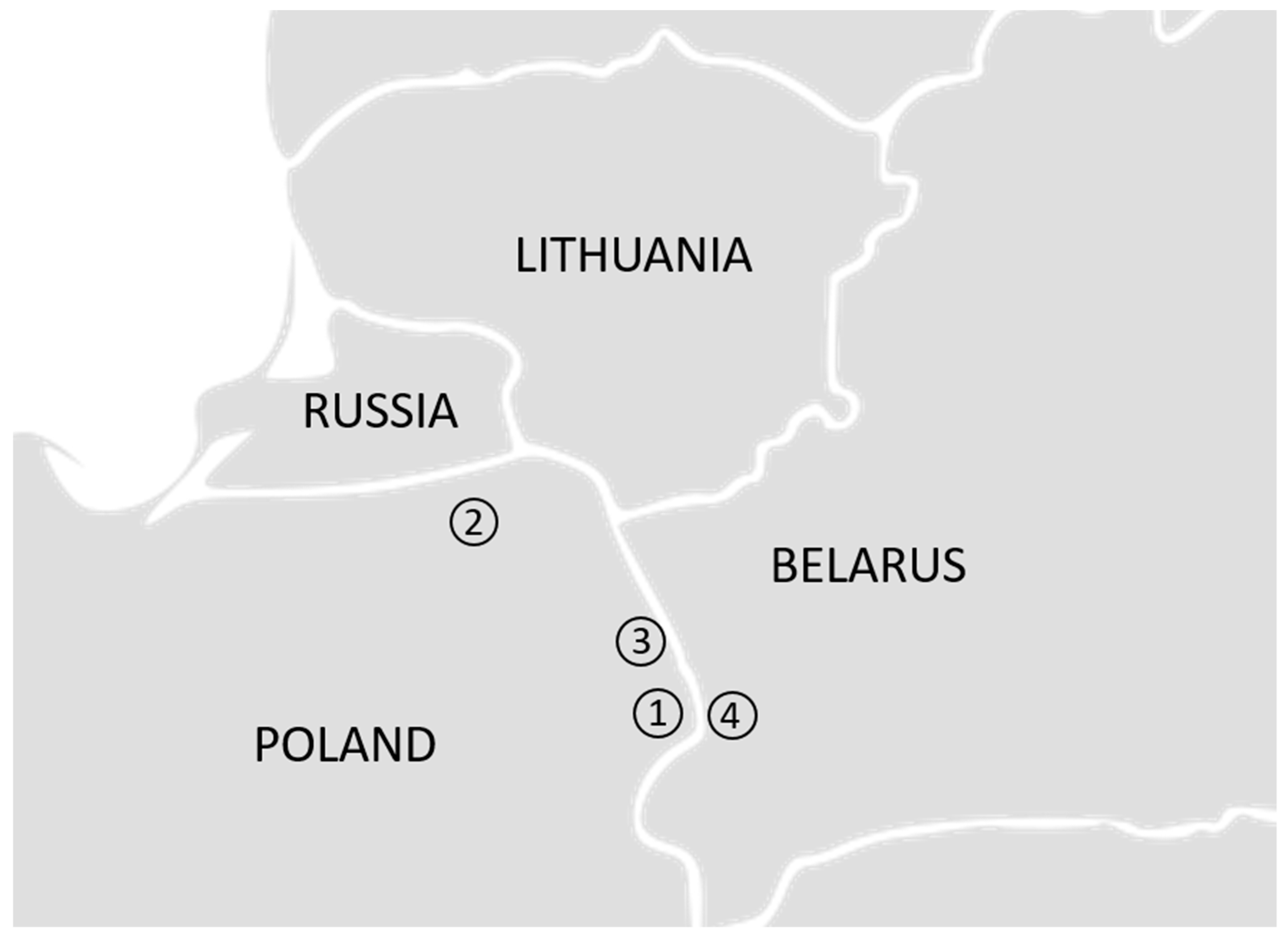
2.1. Samples and DNA Extraction

The material for genetic analyses comprised samples of biological material collected from wisents in the years 2000–2021. Samples were stored at −70 °C in Wisent Genes Bank organized by Department of Animal Genetics and Conservation according to the permit (ref. No. WPN-I.6401.90.2014.EB.1) for preserving tissues from a protected species given by Regional Director of Environmental Protection in Warsaw. The biological material was sent by owners or veterinarians and was taken from animals immobilized for other reasons and from all dead individuals. The material consisted of peripheral blood, fragments of soft tissues, and hair bulbs.
Due to the long duration of research and sampling over the years, DNA was isolated using dedicated kits from various manufacturers: DNeasy Blood & Tissue Kit (Qiagen, Hilden, Germany) was used for DNA isolation from blood, soft tissue fragments, and hair bulbs; QuickGene DNA Whole Blood kit S (Kurabo, Osaka, Japan) was used for DNA isolation from blood; QuickGene DNA Tissue kit S (Kurabo, Osaka, Japan) was used for isolation from soft tissues and hair bulbs; GeneMATRIX Quick Blood DNA Purification Kit (EURx, Gdańsk, Poland) was used for isolation from blood; and GeneMATRIX Tissue DNA Purification Kit (EURx, Gdańsk, Poland) was used for isolation from soft tissues and hair bulbs. When Kurabo kits were used, a QuickGene-Mini80 (Kurabo, Osaka, Japan) nucleic acid isolation system was used for isolation. All procedures were performed following the protocols provided by the manufacturer. The isolated genetic material was subjected to spectrophotometric analysis using NanoDrop2000 (Thermo Fisher Scientific, Waltham, MA, USA), and the samples that met the requirements regarding quantity and purity (ratio parameters: A260/A280 = 1.8–2.0 and A260/A230 = 2.0–2.2) were subjected to further analysis.
In this study, we analyzed 2177 individuals divided into two genetic lines, i.e., 1220 Lowland (LB) individuals and 957 Lowland–Caucasian (LC) individuals. To our knowledge, this is the first study to cover such a large part of the wisent population. Within the Lowland (LB) line, we analyzed a set of 586 wisents in detail: a total of 252 from the Białowieska herd, 146 from the Borecka herd, 82 from the Knyszyńska herd, and 106 from Belarus. The other LB animals (634) came from Poland (523 samples from 19 herds), Germany (54 samples from 7 herds), and the Netherlands and other countries (67 samples from 6 herds). The samples from the LC line were collected from the Polish Biieszczady herd (295 samples), Germany (477 samples from 64 herds), and Sweden (106 samples from 6 herds), and 79 samples were from 23 herds from other countries.

2.2. Genotyping

Ten microsatellite markers were used for analysis. Markers were divided into two multiplex reaction panels, “55” and “60”, under different PCR conditions. The forward primers of each marker were 5′-fluorescently labeled (Table 2). Polymerase chain reaction (PCR) was performed using 3.5 μL of AmpliTaq Gold™ 360 Master Mix with 0.15 μL of 360 GC Enhancer (Applied Biosystems™), 0.04 μL of each primer at a 10 μM concentration, 1 μL of DNA, and deionized PCR-grade water up to the final volume of 7 μL. The cycling conditions for the amplification of microsatellite markers in the “60” panel were as follows: a temperature of 95 °C for 9 min 30 s; followed by 19 cycles at 95 °C for 30 s, 60 °C for 1 min (touchdown of −0.1 °C per cycle), and 72 °C for 45 s; then, 14 cycles at 95 °C for 30 s, 58 °C for 1 min, and 72 °C for 45 s; final extension step at 60 °C for 30 min. The cycling conditions for the amplification of microsatellite markers in the “55” panel were as follows: a temperature of 95 °C for 9 min 30 s; followed by 29 cycles at 95 °C for 30 s, 58 °C for 1 min, and 72 °C for 1 min; final extension step at 60 °C for 30 min. All PCRs were performed using T3 Thermocycler (Biometra, Göttingen, Germany).
After PCR, samples were 10-fold diluted. To 1 μL of each diluted PCR product, 8.5 μL of Hi-Di™ Formamide and 0.5 μL of GeneScan™ 600 LIZ® Size Standard v2.0 were added before electrophoresis. Capillary electrophoresis was performed with 3500 Genetic Analyzer (Applied Biosystem, Foster City, CA, USA) using a 50 cm capillary array and POP-7™ Polymer. The FragmentAnalysis50_POP7 run module protocol in combination with the G5 dye set was used. The reading of the lengths of the obtained fragments was analyzed using GeneMapper® Software v4.1 (Applied Biosystems, Waltham, MA, USA).

2.3. Statistical Analysis

Allele frequencies, observed (Na) and effective numbers of alleles (Ne), observed heterozygosity (Ho), expected heterozygosity (He), unbiased Nei distances between analyzed populations, and Fst, as well as probability of identity (PI) and probability of identity between related animals (PIsibs), were calculated using GenAlEx version 6.502 software [51]. To evaluate the presence of genetic divergence between populations, Principal Coordinate Analysis (PCA) based on genetic distances was performed using GenAlEx software. PCA data visualization was performed using R studio [52] with the Scatterplot3d package [53].
The Bayesian clustering method implemented in Structure v. 2.3.4 [54] was used to illustrate the population genetic structure. Analysis was performed with the Correlated Allele Frequencies Model and the Admixture Model, with a burn-in period of 105 and 105 Markov Chain Monte Carlo (MCMC) replicates for 10 iterations of each K value (K = 1 to 5). Structure Harvester was used to assess the optimal value of K for this study (inspection of log-likelihood values according to the ΔK method developed by Evanno [55]). The raw Structure output files were combined and visualized using Clumpak v. 1.1 [56].

3. Results

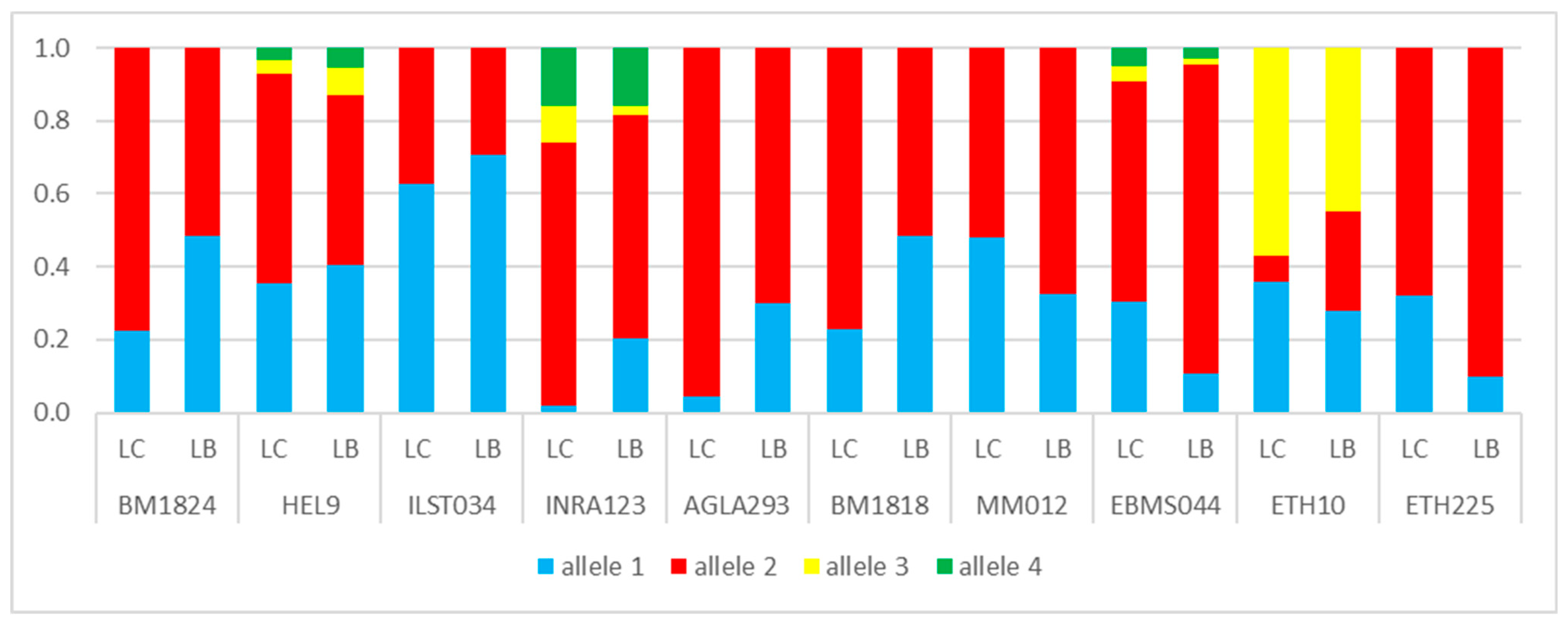
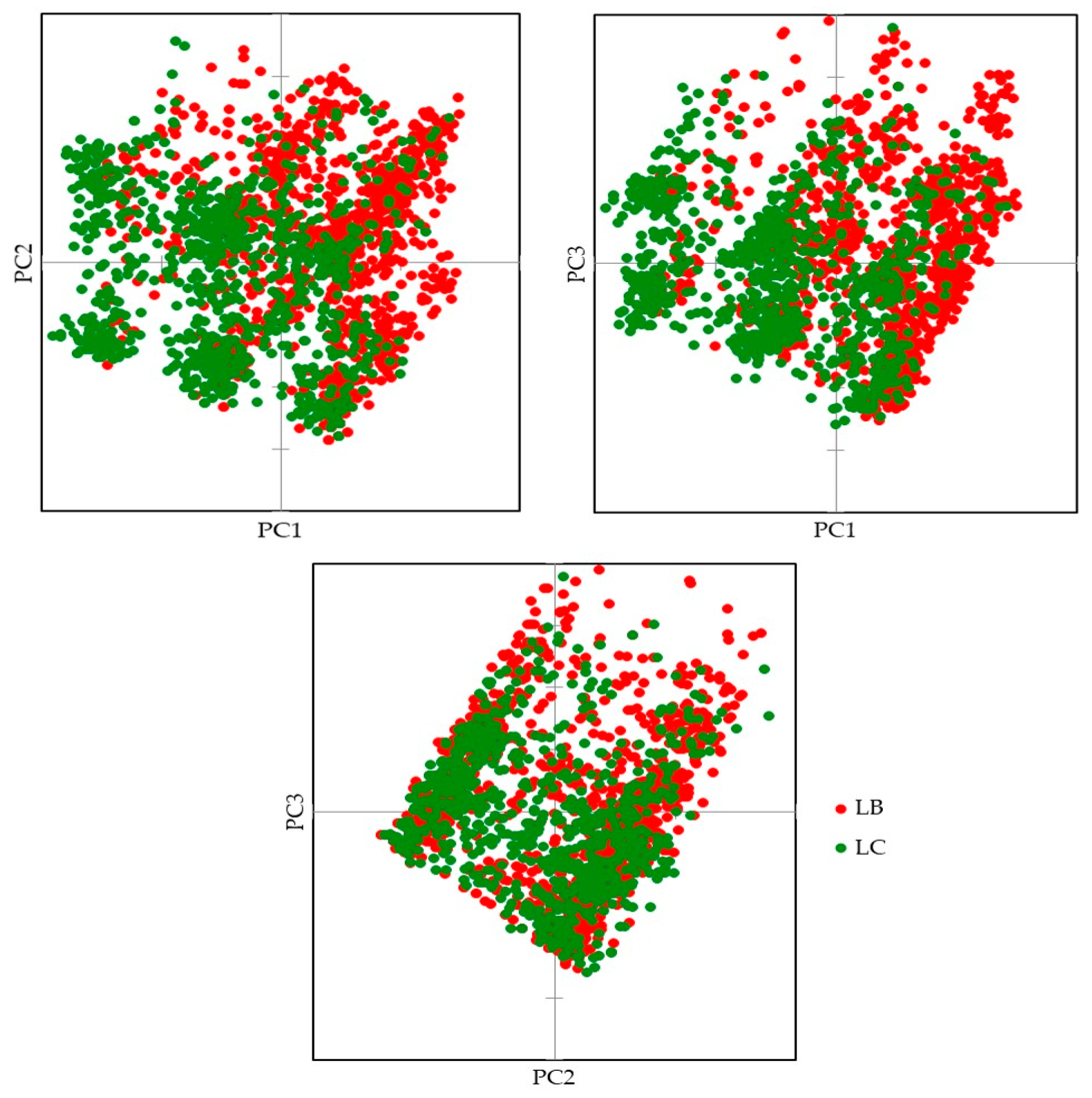
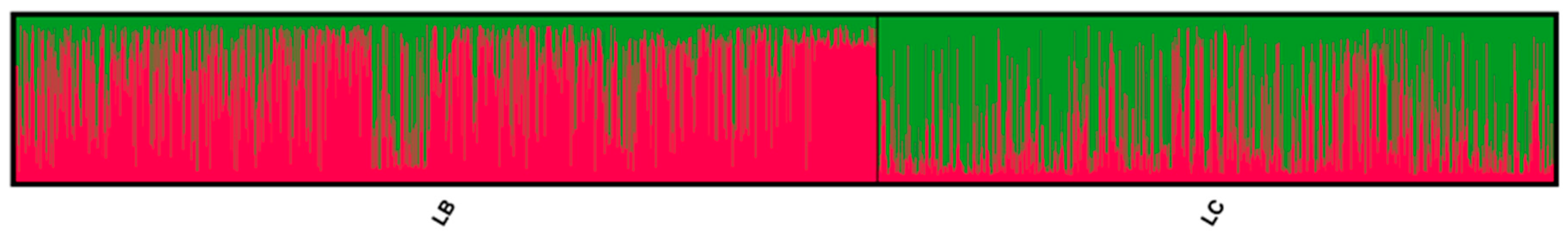
3.1. Genetic Lines—LC vs. LB

The number of alleles was exactly the same at each locus for both genetic lines, from two to four. The frequency within every line was different (Figure 2), but there were no private alleles. The obtained parameters of the genetic lines are presented in Table 3.
On average, heterozygosity was slightly larger in the LC line than in the LB line, but the difference was not large. In locus AGLA293 in the LB line, the polymorphism was very small (Table 2; Figure 2). At the same time, in locus EBNS044 or ETH225, there was a reverse situation, with a smaller value for the LC line than for the LB line. Based on 10 STR loci, the difference between the two genetic lines was very low. The genetic distance between the two lines based on all 10 loci was equal to 7.1%.
When the analysis was performed on all samples without separation into genetic lines, based on 10 microsatellite loci, the probability of identity (PI) for unrelated samples was equal 4.43 × 10⁻⁵, and PIsibs was 7.44 × 10⁻³. For unrelated individuals, the expected number of animals with the same multilocus genotype (calculated as respective probability × population size) was below 1 (0.096), but based on PIsibs, this number was higher (16.196 individuals). The same calculation was made with the assigned genetic lines. For the Lowland line, PI was equal to 1.0 × 10⁻⁴, and for the Lowland–Caucasian line, it equaled 4.5 × 10⁻⁵. The PIsibs parameters were 1.07 × 10⁻² for LB and 7.49 − 10−3 for the LC line. Given the large number of samples (LB—1220; LC—957), the estimated numbers of unrelated individuals with the same multilocus genotype were 0.127 for LB and 0.043 for LC, while based on PIsibs, in LB, 13.058 animals were expected to have the same multilocus genotype, and in LC, this number was lower (7.172 individuals).
The difference between the two genetic lines was not large, as seen in Figure 3, where the results of the PCA analysis are presented. A large part of animals belonging to different lines were genetically very similar, but a little difference was noticeable. The 3d visualization of the PCA results (file lines 3d.gif) is included in the Supplementary Materials.
The Structure results shown in Figure 4 do not indicate a clear division into clusters differentiating genetic lines; however, it is possible to note a certain trend in the estimated proportion of membership to a given cluster. The overall proportion of “red” in the Lowland line was 0.695, and in the Lowland–Caucasian line, it was equal to 0.321. The proportions of “green” were 0.305 in LB and 0.679 in LC. As in the case of PCA, among the animals studied, we can notice those characterized by having a high percentage of belonging to a particular cluster (an extreme percentage of belonging either to the cluster of green or red color), but in both lines, there were also individuals with balanced proportions between the two clusters. However, the ΔK method supports the division into two clusters.

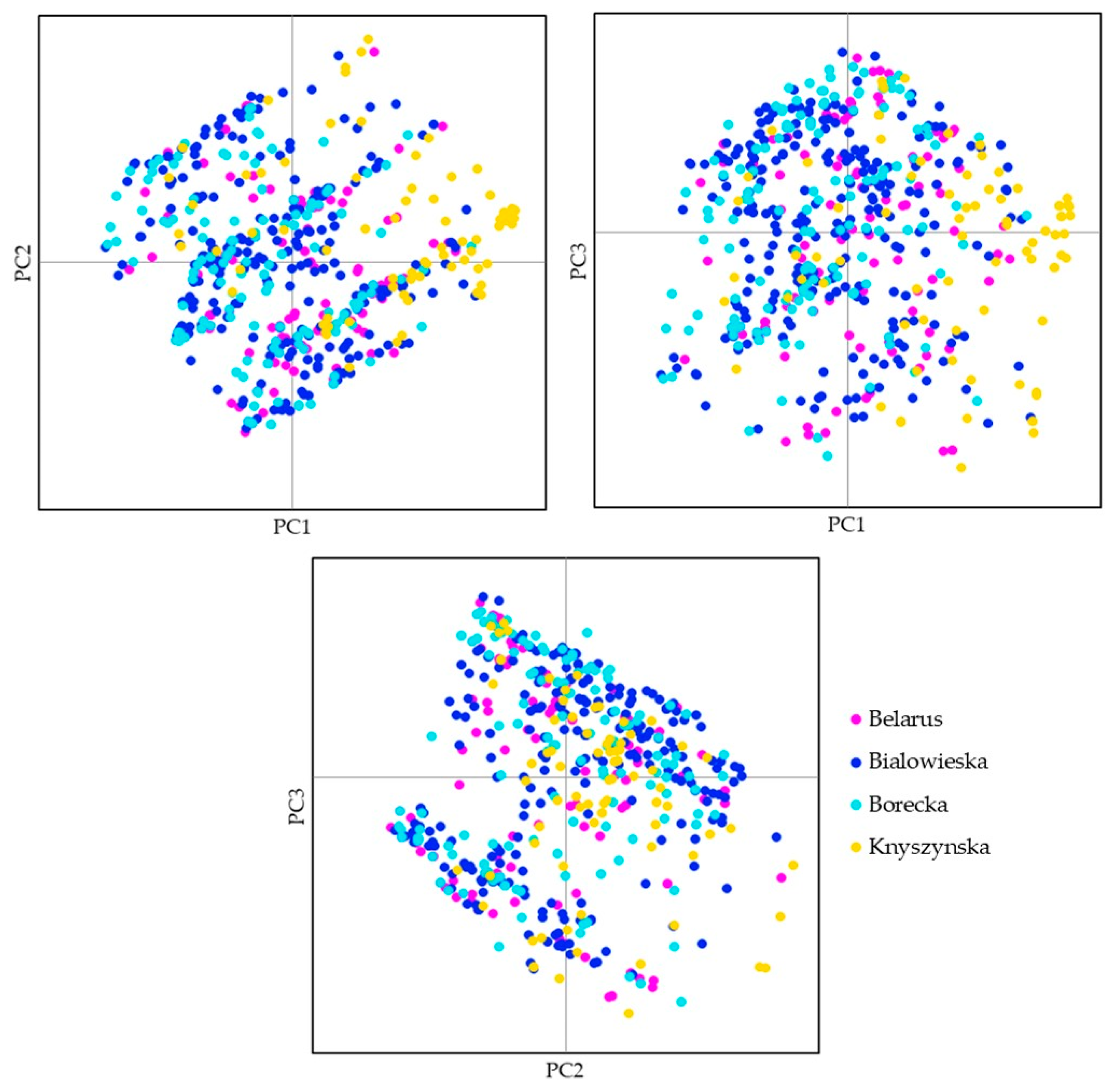
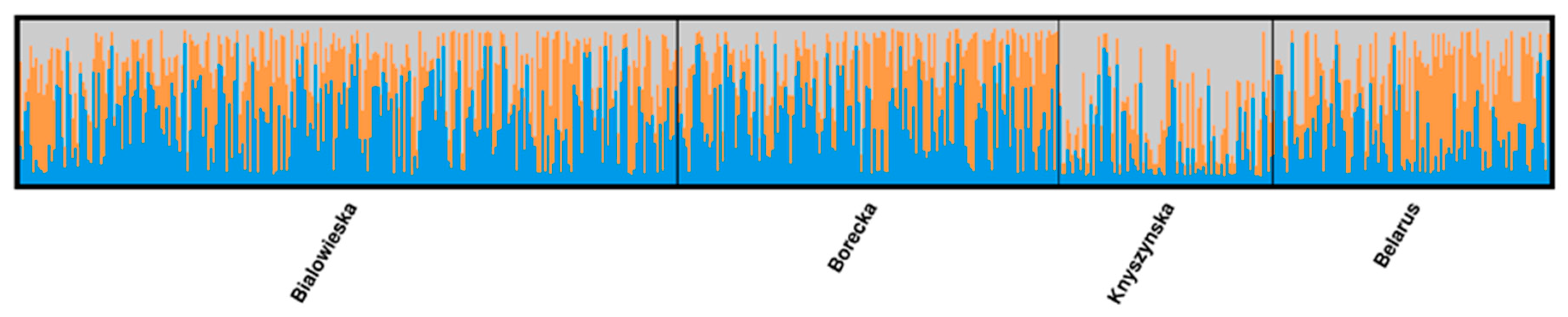
3.2. Four Populations within the Lowland Line (LB)

The results of allele number, and observed and expected heterozygosity of every analyzed Lowland population are presented in Table 4, and distances among all four herds are included in Table 5.
The Belarus population had slightly larger genetic diversity than the other herds from Poland, but compared with Białowieska, the difference was very small. In both populations, Belarus and Białowieska, the effective number of alleles and expected heterozygosity were larger than for the whole Lowland (LB) line (Table 3 and Table 4). The numbers of observed alleles in the Białowieska and Knyszyńska herds were the same, as for the entire LB line. In the Belarus herd, in locus HEL009, there was one allele less than in the LB line, despite the fact that this population had the largest number of effective alleles. Locus AGLA293 in the Borecka population was monomorphic, and in two other loci, HEL009 and INRA123, the number of observed alleles was less than and equal to three. In consequence, the expected heterozygosity was the lowest in this population. In locus MM012, there was very small heterozygosity in the Knyszyńska herd in comparison with the others (Table 4).
The largest distances were found between Knyszyńska and the other populations, and there was a very small difference between populations from Belarus and Białowieska (Table 5). The Knyszyńska population was not in contact with any other population for more than 40 years but was created by releasing animals captured from the Białowieska free-roaming herd and Białowieża reserves. It should be repeated that in the Knyszyńska population, the average heterozygosity was the lowest (Table 4).
In Figure 5, where the visualization of the results of the PCA based on genetic distances is presented, it can be seen that some individuals from the Knyszyńska population are separated from and dissimilar with respect to the rest, while the other populations are mixed together (Figure 5 and Figure 6). The 3d visualization of the PCA results (file LB 3d.gif) is included in the Supplementary Materials.
For a data set including four populations from the Lowland line, the ΔK value indicated three clusters. The Structure graph presented in Figure 6 shows variable participation of individuals in clusters, observed for all populations. However, the herd from Knyszyńska Forest clearly stood out, which was also evident in the PCA analysis.

4. Discussion

Our results are similar to those obtained by other authors. The average number of observed alleles was 2.7 in both lines, and this value corresponds with those reported in other studies [20,23,25] or is larger [19,26]. It is interesting that the number of alleles in the LC line is smaller than that reported in other studies [23,24] (Table 1). This cross-author comparison is difficult, and sometimes even impossible, due to the different loci analyzed, the different sources, and the size of the samples studied. However, it is possible to compare some microsatellites analyzed by different authors, and such locus is BM1824, which was used by almost all authors. In our study, we found two alleles with Ho = 0.440 and 0.294 in the LC and LB lines, respectively. In our studies, the values of the LC line were also larger than those of the LB line, which is the consequence of the larger number of founders of the LC line. Tokarska et al. [23] found three alleles in the Białowieska population and four alleles in LC animals from Russian reserves, but nobody else found more than two alleles. The heterozygosity in our study is smaller than that in other studies, which may be due to the large number of samples. In a group of 60 buffalos (Bison bison), the number of alleles was equal to eight, and heterozygosity was 0.83 [31], but in studies based on a much larger number of samples, those values were smaller [32]. Generally, in Bison bison species analyzed in many studies, the number of alleles and heterozygosity are much larger than those in wisent [57,58]. The polymorphism of buffalo is large enough to use a set of 15 microsatellites for parentage control [31,32] or for checking cattle introgression existence [34]. Our results show a small difference between the two genetic lines of wisent, and as expected, the LC line had a little more genetic variability than the LB line. The PCA graph (Figure 2) shows that both lines were not divided based on ten STR loci. The same can be noticed in Figure 4, where the samples from the two genetic lines are structured in a similar way. In that case, many more markers are needed to identify the genetic lineage. Single Nucleotide Polymorphism (SNP) analysis may be a solution [36], and detailed studies based on SNP results have shown that 30 markers with highly significant differences in allele frequency between genetic lines are sufficient for this purpose [39].
The results of comparing the four Lowland populations are interesting, and for this reason, the number of markers seems to be sufficient. The number of alleles and heterozygosity in all compared populations were similar, but the genetic distances among them show that Knyszyńska differed from the others much more (Figure 5 and Figure 6; Table 5). This is the result of genetic drift and/or the effect of the founding group. The slightly lower number of alleles and heterozygosity values (Table 5) in this isolated population could be symptoms of genetic drift. Using pedigree data, the distance between Knyszyńska and other populations was less than 1% [36], but based on markers, the distance was between 12% and 15%. These values are larger than those obtained in cattle breeds (5% to 10%), but much lower than the distance between Bison bison and Bos taurus breeds (70–78%) [30]. Similar values of genetic distances were found between different populations of chamois (Rupicapra spp.) [29]. The Knyszyńska population was different from all other studied groups, but populations from Belarus and Białowieża were close to each other. This result is opposite to that obtained by [23], who concluded that the Belarusian population is no longer Lowland and is different from the Białowieska herd in Poland. This conclusion is not supported by our results, nor the results obtained in other studies [25,26]. Those two populations are at a very small geographic distance and have come into contact with each other before the border fence was built, so similarity is to be expected. As mentioned, the Knyszynska population was found to be different because of the founder effect and/or genetic drift. The impact of the released animals is unknown. Geographical isolation for more than five generations and the small size of this population could also have caused genetic drift. Such differences are important in species management and could help in preserving genetic variability in the species.

5. Conclusions

By using a set of ten microsatellites, it is not possible to recognize the genetic line of a sampled animal within the species Bison bonasus. Nevertheless, this number of markers could be efficient in presenting differences among herds, as for the four chosen free-roaming populations. Detailed genetic monitoring must be based on a larger set of markers. We prove that a large sample set and a small number of markers could bias the genetic structure comparison.

Supplementary Materials

The following supporting information can be downloaded at: https://www.mdpi.com/article/10.3390/d15030399/s1. The 3d visualization of the PCA results.

Author Contributions

Conceptualization, W.O.; methodology, Z.N.-Ż. and M.W.; validation, Z.N.-Ż. and M.W.; formal analysis, M.K. and M.P.-T.; investigation, M.W. and W.O.; resources, W.O.; data curation, Z.N.-Ż.; writing—original draft preparation, W.O.; writing—review and editing, M.W., M.K. and W.O.; visualization, M.W. and M.P.-T.; supervision, W.O.; project administration, W.O.; funding acquisition, W.O. All authors have read and agreed to the published version of the manuscript.

Funding

This research was partly funded by Forest Fund (Poland), grant number OR.271.3.10.2017.

Institutional Review Board Statement

Not applicable.

Data Availability Statement

The data presented in this study are available upon request from the corresponding author.

Acknowledgments

This study would not have been possible without the commitment of breeders and veterinarians directly involved in wisent conservation. We thank Julia and Katherine Rossi for their kind improvement of the English language.

Conflicts of Interest

The authors declare no conflict of interest.

References

  1. Pucek, Z.; Belousova, I.P.; Krasińska, M.; Krasiński, Z.A.; Olech, W. European Bison Status Survey and Conservation Action Plan; IUCN The World Conservation Union: Gland, Switzerland, 2004; pp. 1–49. [Google Scholar]
  2. Krasińska, M.; Krasiński, Z.A. European Bison–Nature Monograph; Springer: Berlin/Heidelberg, Germany, 2013; pp. 1–379. [Google Scholar]
  3. Krasiński, Z.A. Free-living European bison. Acta Theriol. 1967, 12, 391–405. [Google Scholar] [CrossRef] [Green Version]
  4. Krasiński, Z.A.; Krasińska, M. Free ranging European bison in Borecka Forest. Acta Theriol. 1992, 37, 301–317. [Google Scholar] [CrossRef] [Green Version]
  5. Krasiński, Z.A.; Krasińska, M.; Leniec, H. Żubry w Puszczy Knyszyńskiej. Park. Nar. I Rezerw. Przyr. 1994, 13, 107–114. (In Polish) [Google Scholar]
  6. Kozlo, P. Analysis of reintroduction and formation of European bison populations in Belarus. Eur. Bison Conserv. Newsl. 2013, 6, 21–36. [Google Scholar]
  7. Raczynski, J.; Bołbot, M. European Bison Pedigree Book 2021; Białowieski National Park: Białowieża, Poland, 2022; pp. 1–80. [Google Scholar]
  8. Olech, W.; Perzanowski, K. European Bison (Bison bonasus) Strategic Species Status Review 2020; IUCN SSC Bison Specialist Group and European Bison Conservation Center: Warsaw, Poland, 2022; pp. 1–148. [Google Scholar]
  9. Slatis, H.M. An analysis of inbreeding in the European bison. Genetics 1960, 45, 275–287. [Google Scholar] [CrossRef] [PubMed]
  10. Olech, W. The participation of ancestral genes in the existing population of European bison. Acta Theriol. 1989, 34, 397–407. [Google Scholar] [CrossRef] [Green Version]
  11. Olech, W. The number of ancestors and their contribution to European bison (Bison bonasus L.) population. Ann. Warsaw Agric. Univ. Anim. Sci. 1999, 35, 111–117. [Google Scholar]
  12. Olech, W. The Influence of Individual and Maternal Inbreeding on the Survival of European Bison Calves; Warsaw University of Life Sciences: Warsaw, Poland, 2003; pp. 1–78. (In Polish) [Google Scholar]
  13. Olech, W. The analysis of European bison genetic diversity using pedigree data. In Health Threats for the European Bison Particularly in Free-Roaming Populations in Poland; Kita, J., Anusz, K., Eds.; The SGGW Publishers: Warszawa, Poland, 2006; pp. 205–236. [Google Scholar]
  14. Olech, W.; Perzanowski, K. A genetic background for reintroduction program of the European bison in the Carpathians. Biol. Conserv. 2002, 108, 221–228. [Google Scholar] [CrossRef]
  15. Olech, W. The changes of founders’ numbers and their contribution to the European bison population during 80 years of species’ restitution. Eur. Bison Conserv. Newsl. 2009, 2, 54–60. [Google Scholar]
  16. Hartl, G.B.; Pucek, Z. Genetic depletion in the European bison (Bison bonasus) and the significance of electrophoretic heterozygosity for conservation. Conserv. Biol. 1994, 8, 167–174. [Google Scholar] [CrossRef]
  17. Gębczyński, M.; Tomaszewska-Gruszkiewicz, K. Genetic variability in the European bison. Biochem. Syst. Ecol. 1987, 15, 285–288. [Google Scholar] [CrossRef]
  18. Burzyńska, B.; Olech, W.; Topczewski, J. Phylogeny and genetic variation of the European bison Bison bonasus based on mitochondrial DNA D-loop sequences. Acta Theriol. 1999, 44, 253–262. [Google Scholar] [CrossRef] [Green Version]
  19. Gralak, B.; Krasińska, M.; Niemczewski, C.; Krasiński, Z.A.; Żurkowski, M. Polymorphism of bovine microsatllite DNA sequences in the lowland European bison. Acta Theriol. 2004, 49, 449–456. [Google Scholar] [CrossRef]
  20. Luenser, K.; Fickel, J.; Lehnen, A.; Speck, S.; Ludwig, A. Low level of genetic variability in European bison (Bison bonasus) from Bialowieża National Park in Poland. Eur. J. Wildl. Res. 2005, 51, 84–87. [Google Scholar] [CrossRef]
  21. Roth, T.; Pfeiffer, I.; Weising, K.; Brenig, B. Application of bovine microsatellite markers for genetic diversity analysis of European bison (Bison bonasus). J. Anim. Breed. Genet. 2006, 123, 406–409. [Google Scholar] [CrossRef]
  22. Łopienska, M.; Nowak, Z.; Charon, K.M.; Olech, W. A comparison of polymorphism of DQA genes in European bison belonging to two genetic lines: Lowland and Lowland-Caucasian. Ann. Wars. Univ. Life Sci. SGGW Anim. Sci. 2011, 49, 93–102. [Google Scholar]
  23. Tokarska, M.; Bunevich, A.N.; Demontis, D.; Sipko, T.; Perzanowski, K.; Baryshnikov, G.; Kowalczyk, R.; Voitukhovskaya, Y.; Wójcik, J.M.; Marczuk, B.; et al. Genes of the extinct Caucasian bison still roam the Białowieża Forest and are the source of genetic discrepances between Polish and Belarusian populations of the European bison. Bison bonasus. Biol. J. Linn. Soc. 2015, 114, 752–763. [Google Scholar] [CrossRef] [Green Version]
  24. Dotsev, A.V.; Aksenova, P.V.; Volkova, V.V.; Kharzinova, V.R.; Kostyunina, O.V.; Mnatsekanov, R.A.; Zinovieva, N.A. Study of Allele Pool and Genetic Structure of Russian Population of Lowland-Caucasian Line of European Bison (Bison bonasus). Russ. J. Genet. Appl. Res. 2018, 8, 31–36. [Google Scholar] [CrossRef]
  25. Homel, K.V.; Sliwinska, A.A.; Valnisty, A.A.; Nikifirov, M.E. New data on the genetic diversity of European bison (Bison bonasus) in Belarus. Theriol. Ukr. 2020, 19, 45–53. [Google Scholar] [CrossRef]
  26. Kostyunina, O.V.; Mikhailova, A.D.; Dotseva, A.V.; Zemlyanko, I.I.; Volkova, V.V.; Fornara, M.S.; Akopyana, N.A.; Kramarenko, A.S.; Okhlopkove, I.M.; Aksenova, P.V.; et al. Comparative Genetic Characteristics of the Russian and Belarusian Populations of Wisent (Bison bonasus), North American Bison (Bison bison) and Cattle (Bos taurus). Cytol. Genet. 2020, 54, 116–123. [Google Scholar] [CrossRef]
  27. Nguye, T.T.; Genini, S.; Menetrey, F.; Malek, M.; Vogeli, P.; Goe, M.R.; Stranzinger, G. Application of bovine microsatellite markers for genetic diversity analysis of Swiss yak (Poephagus grunniens). Anim. Genet. 2005, 36, 484–489. [Google Scholar] [CrossRef] [PubMed]
  28. Mukherjee, S.; Mukherjee, A.; Kumar, S.; Verma, H.; Bhardwaj, S.; Togla, O.; Joardar, S.N.; Longkumer, I.; Mech, M.; Khate, K.; et al. Genetic Characterization of Endangered Indian Mithun (Bos frontalis), Indian Bison/Wild Gaur (Bos gaurus) and Tho-tho Cattle (Bos indicus) Populations Using SSR Markers Reveals Their Diversity and Unique Phylogenetic Status. Diversity 2022, 14, 548. [Google Scholar] [CrossRef]
  29. Crestanello, B.; Pechioli, E.; Vernesi, C.; Mona, S.; Martinkova, N.; Janiga, M.; Hauffe, H.C.; Bertorelle, G. The genetic impact of translocations and habitat fragmentation in chamois (Rupicapra) spp. J. Hered. 2009, 100, 691–708. [Google Scholar] [CrossRef] [Green Version]
  30. Mommens, G.; Peelman, L.J.; Van Zeveren, A.; D’Ieteren, G.; Wissocq, N. Microsatellite variation between an African and five European taurine breeds results in a geographical phylogenetic tree with a bison outgroup. J. Anim. Breed. Genet. 1999, 116, 325–330. [Google Scholar] [CrossRef]
  31. Mommens, G.; Zeveren, A.; Peelman, L.J. Effectiveness of bovine microsatellites in resolving paternity cases in American bison, Bison bison L. Anim. Genet. 1998, 29, 12–18. [Google Scholar] [CrossRef]
  32. Schnabel, R.D.; Ward, T.J.; Derr, J.N. Validation of 15 microsatellites for parentage testing in North American bison, Bison bison and domestic cattle. Anim. Genet. 2000, 31, 360–366. [Google Scholar] [CrossRef] [Green Version]
  33. Halbert, N.; Gogan, P.J.P.; Hedrick, P.W.; Wahl, J.M.; Derr, J.N. Genetic Population Substructure in Bison at Yellowstone National Park. J. Hered. 2012, 103, 360–370. [Google Scholar] [CrossRef] [Green Version]
  34. Halbert, N.D.; Derr, J.N. A Comprehensive Evaluation of Cattle Introgression into US Federal Bison Herds. J. Hered. 2007, 98, 1–12. [Google Scholar] [CrossRef] [Green Version]
  35. Ranglack, D.H.; Dobson, L.R.; Du Toit, J.H.; Derr, J. Genetic Analysis of the Henry Mountains Bison Herd. PLoS ONE 2015, 10, e0144239. [Google Scholar] [CrossRef] [Green Version]
  36. Tokarska, M.; Marshall, T.; Kowalczyk, R.; Wójcik, J.M.; Pertoldi, C.; Kristensen, T.N.; Loeschecke, V.; Gregersen, V.R.; Bendixen, C. Effectiveness of microsatellite and SNP markers for parentage and identity analysis in species with low genetic diversity: The case of European bison. Heredity 2009, 103, 326–332. [Google Scholar] [CrossRef] [Green Version]
  37. Kamiński, S.; Olech, W.; Oleński, K.; Nowak, Z.; Ruść, A. Single nucleotide polymorphisms between two lines of European bison (Bison bonasus) detected by the use of Illumina Bovine 50 K BeadChip. Conserv. Genet. Resour. 2012, 4, 311–314. [Google Scholar] [CrossRef] [Green Version]
  38. Wojciechowska, M.; Nowak, Z.; Gurgul, A.; Olech, W.; Drobik, W.; Szmatoła, T. Panel of informative SNP markers for two genetic lines of European bison: Lowland and Lowland–Caucasian. Anim. Biodivers. Conserv. 2017, 40, 17–25. [Google Scholar] [CrossRef] [Green Version]
  39. Wojciechowska, M.; Puchała, K.; Nowak-Życzyńska, Z.; Perlińska-Teresiak, M.; Kloch, M.; Drobik-Czwarno, W.; Olech, W. From Wisent to the Lab and Back Again—A Complex SNP Set for Population Management as an Effective Tool in European Bison Conservation. Diversity 2023, 15, 116. [Google Scholar] [CrossRef]
  40. Oleński, K.; Kamiński, S.; Tokarska, M.; Hering, D.M. Subset of SNPs for parental identification in European bison Lowland-Białowieża line (Bison bonasus bonasus). Conserv. Genet. Resour. 2018, 10, 73–78. [Google Scholar] [CrossRef] [Green Version]
  41. Grzegrzółka, B.; Olech, W.; Krasiński, Z.A. Struktura genetyczna wolnych stad żubrów nizinnych w Polsce. Park. Nar. I Rezerw. Przyr. 2004, 23, 665–677. (In Polish) [Google Scholar]
  42. Krasińska, M.; Krasiński, Z.A.; Bunevich, A.N. Spatial distribution of the European bison population in Polish and Belarussian parts of Białowieża Forest. In Proceedings of the Conference European Bison Conservation, Bialowieza, Poland, 30 September–2 October 2004; p. 73. [Google Scholar]
  43. Barendse, W.; Armitage, S.M.; Kossarek, L.M.; Shalom, A.; Kirkpatrick, B.W.; Ryan, A.M.; Clayton, D.; Li, L.; Neibergs, H.L.; Zhang, N.; et al. A genetic linkage map of the bovine genome. Nat. Genet. 1994, 6, 227–235. [Google Scholar] [CrossRef]
  44. Kaukinen, J.; Varvio, S.L. Eight polymorphic bovine microsatellites. Anim. Genet. 1993, 24, 148. [Google Scholar] [CrossRef]
  45. FAO. Global Project for the Maintenance of Domestic Animal Genetic Diversity (MoDAD)–Draft Project Formulation Report; FAO: Rome, Italy, 1995. [Google Scholar]
  46. Vaiman, D.; Mercier, D.; Moazami-Goudarzi, K.; Eggen, A.; Ciampolini, R.; Lépingle, A.; Velmala, R.; Kaukinen, J.; Varvio, S.L.; Martin, P.; et al. A set of 99 cattle microsatellites: Characterization, synteny mapping, and polymorphism. Mamm. Genome 1994, 5, 288–297. [Google Scholar] [CrossRef]
  47. Mommens, G.; Coppieters, W.; Van de Weghe, A.; Van Zeveren, A.; Bouquet, Y. Dinucleotide repeat polymorphism at the bovine MM12E6 and MM8D3 loci. Anim. Genet. 1994, 25, 368. [Google Scholar] [CrossRef] [PubMed]
  48. Bishop, M.D.; Kappes, S.M.; Keele, J.W.; Stone, R.T.; Sunden, S.L.; Hawkins, G.A.; Toldo, S.S.; Fries, R.; Grosz, M.D.; Yoo, J.; et al. A genetic linkage map for cattle. Genetics 1994, 136, 619–639. [Google Scholar] [CrossRef]
  49. Toldo, S.S.; Fries, R.; Steffen, P.; Neibergs, H.L.; Barendse, W.; Womack, J.E.; Hetzel, D.J.; Stranzinger, G. Physically mapped, cosmid-derived microsatellite markers as anchor loci on bovine chromosomes. Mamm. Genome 1993, 4, 720–727. [Google Scholar] [CrossRef] [PubMed]
  50. Steffen, P.; Eggen, A.; Dietz, A.B.; Womack, J.E.; Stranzinger, G.; Fries, R. Isolation and mapping of polymorphic microsatellites in cattle. Anim. Genet. 1993, 24, 121–124. [Google Scholar] [CrossRef] [PubMed]
  51. Peakall, R.; Smouse, P.E. GenAlEx 6.5: Genetic analysis in Excel. Population genetic software for teaching and research_an update. Bioinformatics 2012, 28, 2537–2539. [Google Scholar] [CrossRef] [Green Version]
  52. RStudio Team 2022, RStudio: Integrated Development Environment for R. RStudio, PBC, Boston, MA URL. Available online: http://www.rstudio.com/ (accessed on 2 March 2022).
  53. Ligges, U.; Mächler, M. Scatterplot3d–an R Package for Visualizing Multivariate Data. J. Stat. Softw. 2003, 8, 1–20. [Google Scholar] [CrossRef] [Green Version]
  54. Evanno, G.; Regnaut, S.; Goudet, J. Detecting the number of clusters of individuals using the software STRUCTURE: A simulation study. Mol. Ecol. 2005, 14, 2611–2620. [Google Scholar] [CrossRef] [PubMed] [Green Version]
  55. Earl, D.A.; von Holdt, B.M. STRUCTURE HARVESTER: A website and program for visualizing STRUCTURE output and implementing the Evanno method. Conserv. Gen. Res. 2012, 4, 359–361. [Google Scholar] [CrossRef]
  56. Kopelman, N.M.; Mayzel, J.; Jakobsson, M.; Rosenberg, N.A.; Mayrose, I. CLUMPAK: A program for identifying clustering modes and packaging population structure inferences across K. Mol. Eco. Res. 2015, 15, 1179–1191. [Google Scholar] [CrossRef] [Green Version]
  57. Cronin, M.A.; MacNeil, M.D.; Leeburg, V.; Vu, N.; Blackburn, H.D.; Derr, J. Genetic variation and differentiation of bison (Bison bison)) subspecies’ and cattle (Bos taurus) breeds and subspecies. J. Hered. 2013, 104, 500–509. [Google Scholar] [CrossRef] [Green Version]
  58. Wilson, G.A.; Strobeck, C. The isolation and characterization of microsatellite loci in bison, and their usefulness in other artiodactyls. Anim. Genet. 1999, 30, 226–227. [Google Scholar] [CrossRef]
Figure 1. The four free-roaming populations of wisents: (1) Białowieska (Poland), (2) Borecka, (3) Knyszyńska, and (4) Belarus.
Diversity 15 00399 g001
Figure 2. Frequency of alleles within all 10 loci and two genetic lines (LC and LB).
Diversity 15 00399 g002
Figure 3. Principal Coordinate Analysis (PCA) of 2 genetic lines (Lowland-Caucasian LC and Lowland LB), based on 10 microsatellite markers (PC1 = 18.92%; PC2 = 14.48%; PC3 = 11.67%).
Diversity 15 00399 g003
Figure 4. Results of Bayesian clustering of 2171 individuals from 2 genetic lines. The Structure plot represents the run when K = 2. Individuals are ordered by genetic line, and each of them is represented by a line proportionally divided into color segments. The black line separates individuals from different genetic lines.
Diversity 15 00399 g004
Figure 5. Principal Coordinate Analysis (PCA) of 4 populations, based on 10 microsatellite markers (PC1 = 19.41%; PC2 = 16.15%; PC3 = 13.08%).
Diversity 15 00399 g005
Figure 6. Structure plot that shows the genetic affiliation of LB line individuals from 4 different herds with groups computed by the program. The plot represents the run when K = 3. Individuals are ordered by origin, each represented by a line proportionally divided into color segments. Each color represents one genetic group. Black lines separate the individuals from different herds.
Diversity 15 00399 g006
Table 1. Results of microsatellite locus diversity in wisent Bison bonasus obtained by other authors.
Source of SamplesNumber of SamplesGenetic Line *Number of LociAllelic RichnessObserved HeterozygosityExpected HeterozygosityAuthors
Poland Białowieska22LB211.9050.2410.245Gralak et al., 2004 [19]
Poland Białowieska38LB92.6670.5060.507Luenser et al., 2005 [20]
Poland Białowieska247LB172.7900.2590.279Tokarska et al., 2015 [23]
Belarus48LB172.4700.2830.270Tokarska et al., 2015 [23]
Belarus30LB112.4340.4240.317Homel et al., 2020 [25]
Belarus42LB111.8180.2810.277Kostyunina et al., 2020 [26]
Russia reserves111LC112.1820.3020.286Kostyunina et al., 2020 [26]
Poland Bieszczady and Russia56LC173.2600.3580.392Tokarska et al., 2015 [23]
Russian reserves26LC102.8000.2620.293Dotsev et al., 2018 [24]
German reserves35LC112.3600.4530.447Roth et al., 2006 [21]
* LB—Lowland line; LC—Lowland–Caucasian line.
Table 2. Microsatellite markers with information about source data.
LocusForward Primer Sequence (5′–3′)Reverse Primer Sequence (5′–3′)Fluorescent DyePanelSource
BM1824GAGCAAGGTGTTTTTCCAATCCATTCTCCAACTGCTTCCTTGPET55[43]
HEL009CCCATTCAGTCTTCAGAGGTCACATCCATGTTCTCACCACVIC55[44]
ILST034AAGGGTCTAATGCCACTGGCGACCTGGTTTAGCAGAGAGC6-FAM55[45]
INRA123TCTAGAGGATCCCCGCTGACAGAGAGCAACTCCACTGTGCNED55[46]
MM012CAAGACAGGTGTTTCAATCTATCGACTCTGGGGATGATGT6-FAM55[47]
AGLA293GAAACTCAACCCAAGACAACTCAAGATGACTTTATTCTCCACCTAGCAGAVIC55[31]
BM1818AGCTGGGAATATAACCAAAGGAGTGCTTTCAAGGTCCATGC6-FAM55[48]
EBMS044CCTTGCCACTATTTCCTCCACCAAATGACACATGACAGCCNED60[45]
ETH010GTTCAGGACTGGCCCTGCTAACACCTCCAGCCCACTTTCTCTTCTCNED60[49]
ETH225GATCACCTTGCCACTATTTCCTACATGACAGCCAGCTGCTACTVIC60[50]
Table 3. Genetic parameters of Lowland–Caucasian (LC) and Lowland (LB) lines.
LC LineLB Line
LocusNaNeHoHeNeHoHe
BM182421.9980.4400.5001.5380.2940.350
HEL00942.5680.2410.6112.1890.1730.543
ILST03421.7060.3830.4141.8820.3940.469
INRA12342.2570.6010.5571.7860.5210.440
AGLA29321.7190.3890.4181.0900.0800.083
BM181821.9980.4440.4991.5460.3040.353
MM01221.7830.4020.4391.9970.4210.499
EBMS04441.3770.2040.2742.1680.4520.539
ETH01032.8330.5760.6472.1850.4760.542
ETH22521.2170.1220.1781.7710.3640.435
Mean2.71.9460.3800.4541.8150.3480.425
SE0.30.1590.0490.0460.1110.0440.044
Table 4. Heterozygosity and effective number of alleles in four populations belonging to the Lowland (LB) line.
BiałowieskaBoreckaKnyszyńskaBelarus
NeHoHeNeHoHeNeHoHeNeHoHe
BM18241.630.360.391.370.270.271.840.290.461.750.430.43
HEL0092.170.180.542.340.230.572.140.340.532.520.230.60
ILST0341.630.350.381.290.210.221.540.350.351.950.420.49
INRA1231.870.580.461.720.510.421.870.580.471.530.390.34
AGLA2931.150.140.131.00001.010.010.011.190.130.16
BM18181.670.400.401.430.260.301.880.330.471.760.440.43
MM0121.850.420.461.930.410.481.190.100.161.880.480.47
EBMS0442.420.500.592.200.490.551.740.190.432.440.630.59
ETH0102.090.530.522.090.520.521.290.190.222.330.540.57
ETH2251.960.470.491.960.460.491.450.120.311.760.340.43
Mean1.840.390.441.730.330.381.600.250.341.910.400.45
s.d.0.110.050.040.140.050.060.110.050.050.130.050.04
Table 5. Unbiased Nei distances among analyzed populations (below diagonal) and Fst values (above diagonal).
BelarusBiałowieskaBoreckaKnyszyńska
Belarus-0.80%2.61%7.81%
Białowieska1.39%-1.11%8.21%
Borecka3.14%0.92%-9.85%
Knyszyńska12.06%12.78%15.19%
Disclaimer/Publisher’s Note: The statements, opinions and data contained in all publications are solely those of the individual author(s) and contributor(s) and not of MDPI and/or the editor(s). MDPI and/or the editor(s) disclaim responsibility for any injury to people or property resulting from any ideas, methods, instructions or products referred to in the content.

