Article

Copepod Assemblages in A Large Arctic Coastal Area: A Baseline Summer Study

by
Vladimir G. Dvoretsky
* and
Alexander G. Dvoretsky
Murmansk Marine Biological Institute of the Russian Academy of Sciences (MMBI RAS), 183010 Murmansk, Russia
*
Author to whom correspondence should be addressed.
Diversity 2023, 15(1), 81; https://doi.org/10.3390/d15010081
Submission received: 14 December 2022 / Revised: 3 January 2023 / Accepted: 5 January 2023 / Published: 7 January 2023

Abstract

:
To provide a baseline description of copepod assemblages in the Pechora Sea, an estuarine area with great economical and ecological importance, we conducted a survey during the summer season. A total of 24 copepod taxa were identified in the study, with Acartia longiremis, Calanus finmarchicus, Centropages hamatus, Copepoda nauplii, Eurytemora affinis, Oithona similis, Pseudocalanus spp., and Temora longicornis being the most numerous. The high diversity (Shannon index = 2.51 ± 0.06), density (18,720 ± 3376 individuals m−3) and biomass (89 ± 18 mg dry mass m−3) of copepods were revealed. Populations of common small copepod taxa were dominated by the young stages, indicating spawning, while older copepodites prevailed among medium- and large-sized species, showing that their reproduction occurred before our survey. Cluster analysis indicated three groups of stations that mainly differed in the abundance of particular species. There were clear associations between copepod assemblages and environmental variables. Statistical analyses showed significant correlations between copepod abundance and water temperature or sampling depth, while other factors had a lesser influence. Our results suggest a strong effect of local circulation and currents on the spatial pattern of the copepod assemblages in the study area. This study may be useful for future biomonitoring in the south-eastern Barents Sea.

1. Introduction

The Barents Sea is a high-latitude, shallow continental shelf region and may be considered a transition zone between the North Atlantic Ocean and the Arctic Ocean [1,2]. The southern, western, and south-western parts of the sea are influenced by the warm and saline Atlantic water (AW) flowing as Norwegian Coastal Water from the Norwegian Sea [3]. The northern, north-eastern, and north-western parts of the sea are affected by the less saline, cold waters originating from the Arctic Ocean (ArW). There is a mixing of these two main types of water masses in the central Barents Sea, forming the Polar Front Zone [4]. The climatic conditions and the ice coverage demonstrate clear inter-annual fluctuations and are strongly associated with the intensity of the Atlantic water influx into the Barents Sea [2,4].
Together with AW and ArW, coastal water represents the third main type of water mass present in the Barents Sea [5]. Varying temperature and salinity fluctuations are the primary characteristics of this water mass. Some sub-regions may be divided among the coastal waters [2,3,4]. One of these is the Pechora coastal water recorded in the south-eastern Barents Sea. The oceanography and ecology of the region are defined by the strong discharge of freshwater from the Pechora River so that significant temperature and salinity gradients exist in the coastal area with the lowest salinity and highest temperature in the inshore waters [6,7]. The estuarine zone is large and covers most of the south-eastern Barents Sea.
The Barents Sea is considered one of the most productive regions of the world’s ocean [8]. The maximum primary production is associated with the phytoplankton bloom occurring in spring, with enhanced values in Atlantic water [9,10]. Zooplankton assemblages utilize phytoplankton production and transfer energy to higher trophic levels [11,12]. Many nursery areas for the offspring of commercial fish and shellfish stocks and their spawning are located in the western, southern-western, and southern parts of the sea [2,13,14]. The most important species are herring, cod, haddock, saithe, red king crab, and snow crab [13,14,15]. High fish biomass and production support higher trophic levels, including the minke whale, humpback whale, white-sided dolphin, and white-beaked dolphin [1]. Cod and haddock feed in the Barents Sea from summer to winter and move out of the area and farther south along the Norwegian coast in spring to spawn [15]. Capelin and polar cod represent the main species that spend their whole life-cycle in the Barents Sea [16]. These species are the main plankton-feeding fish in the Barents Sea. In some years, young herring may also play an important role as plankton consumers in Atlantic water (western and southern part of the sea). The south-eastern Barents Sea has a relatively lower fish production than southern areas [7]. Although commercial fishing in the Pechora Sea is very limited and mainly local, some important species inhabit the region, including navaga, polar cod, Pacific herring, and haddock [17].
Moreover, there are other economic human activities in the south-eastern area connected with oil and gas development, shipping, aquaculture, and tourism. For instance, large oil and gas fields are located in the Pechora Sea, and the platform Prirazlomnaya has been in use by the Gazprom Neft Shelf Company since 2013[18]. The exploitation of hydrocarbon resources in the region is associated with offshore drilling, building platforms, and subsea modules, as well as transport of oil and gas condensate. Human activities connected with oil–gas development and shipping along the Northern route may create potential risks for the marine environment, including pollution, contamination, and damage to ecosystems. To assess the environmental health status of marine ecosystems, biotic indicators are often used [19,20,21].
Copepods are considered the most abundant and productive group of mesozooplankton inhabiting marine and estuarine waters worldwide [11,22,23]. Ecologically, they play an important role in pelagic food webs as major prey sources for the larval stages of some key fishery species, many adult planktivorous fish, other plankton animals (hyperiids, medusae, ctenophores), seabirds and marine mammals [11,24]. Additionally, copepods directly affect the downward flux of carbon with fecal pellets, carcasses, and organic matter, linking pelagic and benthic communities [12]. Copepod populations are good indicators of environmental fluctuations [25,26] because copepod responses to various factors quickly, and their response can easily be interpreted [27]. The impacts of stressors on zooplankton are reflected through changes in species distribution and abundance, changes in life-cycle timing, and modified structures of copepod assemblages [27,28].
Studies on the Barents Sea zooplankton have mainly focused on the southern, western, central, and northern regions [12,29,30,31,32,33,34,35,36,37,38,39,40,41,42]. The eastern sector of the sea has been less well studied [29,30,38]. Despite the long history of zooplankton investigations in the Pechora Sea, there few studies dealing with copepod communities are available to an international audience [29,43].
In the present paper, we tested the hypothesis that there would be a clear delineation between copepod assemblages, associated with environmental conditions from inshore to offshore waters. We also aimed to study the diversity, abundance, biomass, and population structure of common copepods to provide baseline data that may be useful for the future monitoring of pelagic ecosystems in the south-eastern Barents Sea.

2. Material and Methods
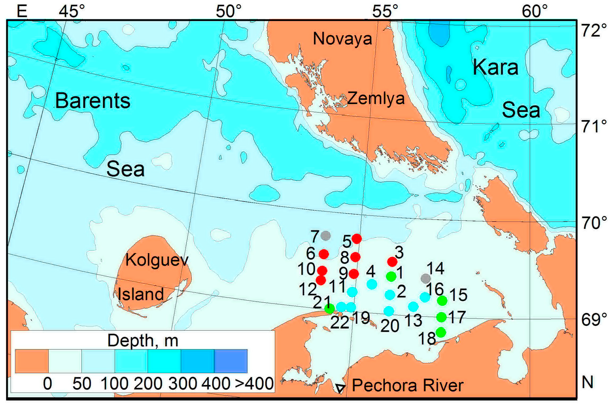
2.1. Sampling

Zooplankton were sampled using a Juday net (0.1 m2, 168 μm mesh size, total length 2 m) under a vertical tow from the bottom to the surface at 22 stations during a cruise of RV Dalnie Zelentsy in the south-eastern Barents Sea (Figure 1, Table 1).
The filtered volume was calculated by multiplying the distance traveled by the net and the net mouth area. We assumed the filtration efficiency of the net to be 100% because the speed of tows was 1–1.2 m s−1 and the mouth angles of the net were nearly 0° from vertical at all sampled stations. Zooplankton samples were caught regardless of the time of day and immediately preserved in a buffered formalin seawater solution with a final concentration of 4%. A CTD profiler (Seabird SBE 19 plus SEACAT) was used to record water temperature and salinity at each station prior to zooplankton sampling. Discrete water samples for chlorophyll a were collected using Niskin bottles attached to a rosette sampler from sampling depths spread throughout the water column.

2.2. Processing

Mean temperature and salinity were calculated for each station. Water samples (0.5 L) for the determination of chlorophyll a were filtered onto 0.6 μm polycarbonate membranes. Filtration was performed using a low-vacuum compressor. Pigment concentrations were measured using the spectrophotometric method [44] and the standard procedure [45] after 24 h extraction in 90% acetone at −5 °C in the dark. Chlorophyll a concentrations were expressed as mg m−3.
In the laboratory, the preserved zooplankton samples were washed to remove formaldehyde and diluted with a pipette splitter in fractions of 1/10 or 1/20 containing 200–500 specimens. Copepods were sorted, identified to the lowest possible taxon, measured, and counted in a Bogorov tray under an MBS-10 stereomicroscope at 32×–56× magnification. The relevant copepod taxonomic literature [22,46,47] was used for identification. Copepod abundance/density was calculated on the basis of the volume of water filtered by the net and the fraction of the sample that was counted. Calanus finmarchicus and C. glacialis were separated on the basis of their prosome lengths using available data from the literature [48,49]. Some recent publications have shown that prosome length measurements should be updated by DNA identification to correctly identify Calanus spp. [50]. However, identification based on body length and other morphological criteria is a preferable routine technique in cases where a large number of copepods are analyzed. Specimens of Pseudocalanus species were distinguished according to Frost [51], while Pseudocalanus copepodites I–IV were combined into one group due to their morphological similarity. Copepod abundance was expressed as number per 1 m3 or 1 m2 (ind. m−3/ind. m−2). Copepod biomass was calculated as the product of the abundance and the individual mass or developmental stage of each species. The individual masses were obtained from published length-weight regressions (Table 2).
Carbon mass was converted to dry mass (DM) by applying a conversion factor: 1 mg C = 2 mg DM [62]. The plankton net used in our study may undersample small taxa (e.g., Copepoda nauplii, Oithona similis, and Triconia spp.). However, we calculated the abundance/biomass of these taxa to show their density and estimate their relative abundance/biomass.

2.3. Data Analysis

Copepod assemblages were classified using multivariate methods. Species abundances (ind. m−3) were square-root-transformed and the percentage similarities between stations were calculated using the Bray–Curtis similarity index [63]. Hierarchical clustering with a group-average linkage method, based on sample similarities, was performed. SIMPER analysis was used to identify the copepod taxa contributing to the total dissimilarity within cluster groups. The differences in abundance data between clusters were tested with ANOSIM, a standard procedure in the Primer 5 software package. The diversity of copepod assemblages was assessed using the Shannon index [64], calculated from the species abundance: H1′ = −Σpilog2pi where i is the sample number and pi is the proportion of the total count (abundance or biomass) represented by the ith species. Pielou’s evenness was calculated as J = H/log2S [65], where S is the total number of taxa in a sample. To test for differences in environmental variables, copepod biomass, diversity, and evenness, we used Kruskal–Wallis tests or one-way ANOVA when the data demonstrated normal distribution.
Detrended correspondence analysis was performed to analyze the modality of the taxa distribution. The total observed inertia was <2.5, so a predominance of linear species response curves could be expected. Therefore, we chose redundancy analysis (RDA) to model the species abundance (ind. m−3), richness, and diversity as functions of the measured environmental variables [66]. Environmental factors in RDA included latitude, longitude, mean and surface water temperature, mean and surface salinity, mean and surface chlorophyll a concentration, depth of sampling, mean abundance of carnivorous macrozooplankton (ind. m−3) at the sampling layer. The chlorophyll a concentration was used as a proxy for potential food sources for copepods. The macrozooplankton density was applied to reveal the possible impact of predator pressure on the copepod assemblages. Data on the macrozooplankton for the same area and the same period were obtained from a previously published report [40]. The densities of the copepods and macrozooplankton taxa were square-root transformed prior to the analysis to obtain a normal distribution of data. Forward selection of the environmental variables included in the model was used to reveal the factors most closely associated with the spatial pattern of the copepod communities, and to measure their relative importance. The statistical significance was tested with Monte Carlo permutation tests (999 unrestricted permutations) (p < 0.05) in the CANOCO package for Windows v4.5 [67]. Additionally, Pearson’s correlation analysis was used to find possible relationships between the total abundances of common taxa and environmental variables during the sampling period after testing the data for normality and heterogeneity. Contours of water temperature, salinity, and chlorophyll a concentration, as well as integrated copepod abundance (ind. m−2), biomass (gDM m−2), diversity, and evenness, were produced from gridded data using the kriging method with MapViewer v7.0 software. All mean values are presented with standard errors (±SE).

3. Results

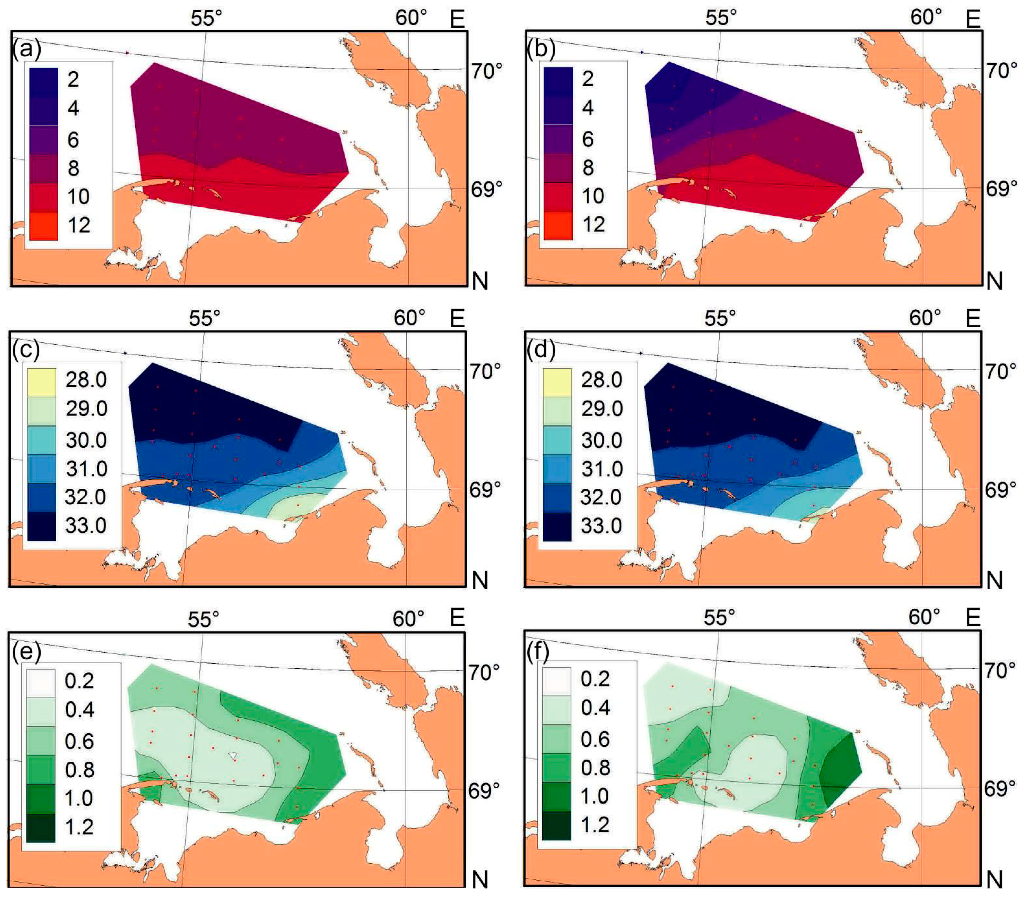
3.1. Environmental Conditions

A distinct sub-surface layer of low-temperature water between 20 and 70 m was recorded at relatively deepwater stations located in the northern part of the study area. A thermocline was absent at the southernmost stations, where there were no variations in the vertical distribution of water temperature. In general, the surface water temperature did not significantly differ between the stations (Figure 2a) while the mean temperature decreased from the north to the south (Figure 2b).
Surface salinity ranged from 28.52 (St. 18) to 33.78 (St. 7) (Figure 2c). The low surface salinities observed in the southern part of the study area reflected the strong influence of freshwater discharge from the river run-off. Mean salinity demonstrated the same pattern, i.e., it decreased northward (Figure 2d). The horizontal patterns of chlorophyll a concentrations during the investigation period are shown in Figure 2e,f. High concentrations of chlorophyll a in the water column were recorded at stations in the western and eastern parts of the study area. These locations were characterized by total chlorophyll a concentrations higher than 1 mg m−3. Minimal surface chlorophyll a was found in the central part of the study area (Figure 2e). The lowest mean chlorophyll a concentrations were registered at stations in the central and northern regions (Figure 2f). The abundance of carnivorous macrozooplankton (medusae, crustaceans, chaetognaths, ctenophores) varied from 0 to 439 ind. m−3, with minimum values in the south-eastern and north-western locations [40].

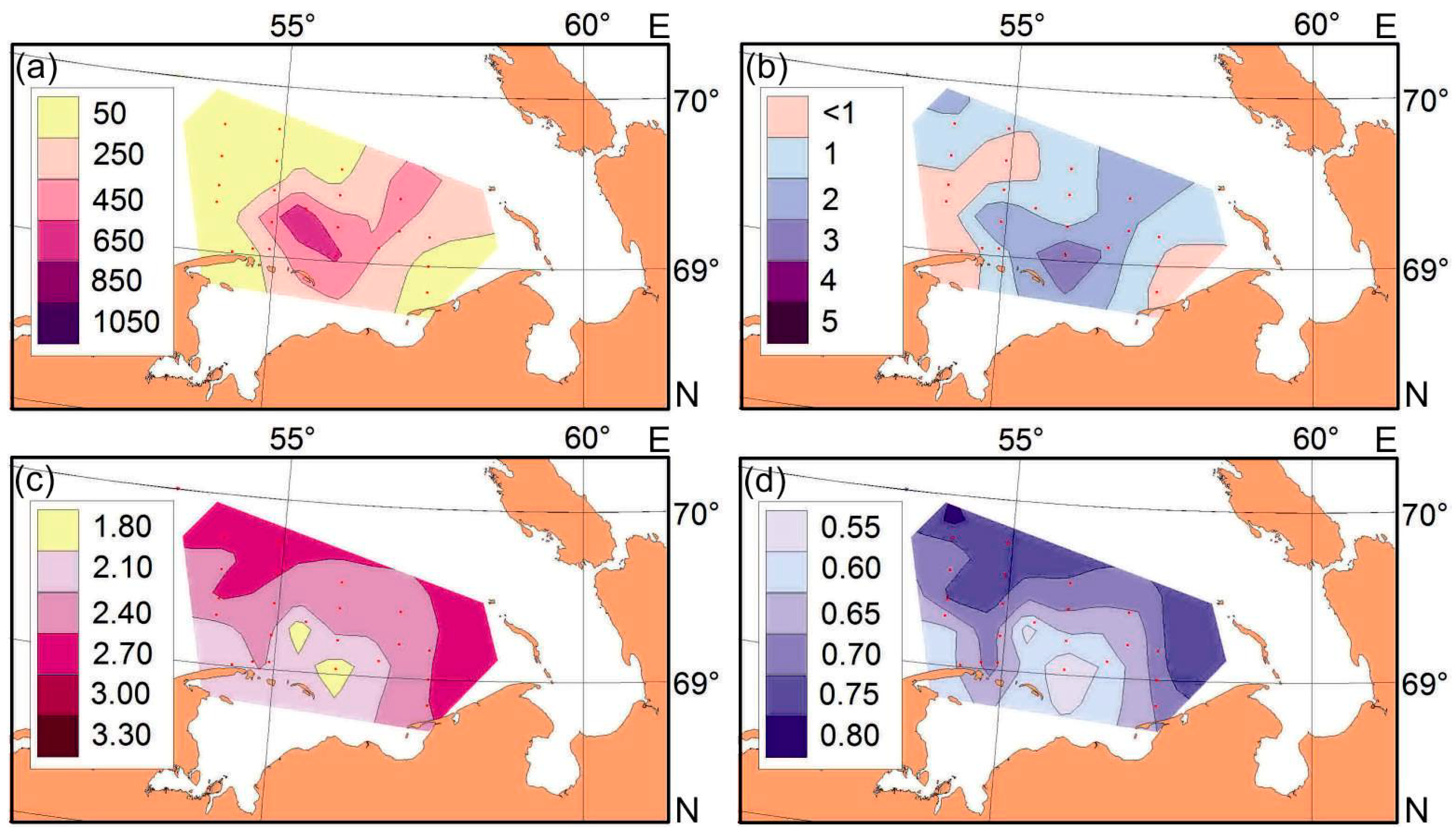
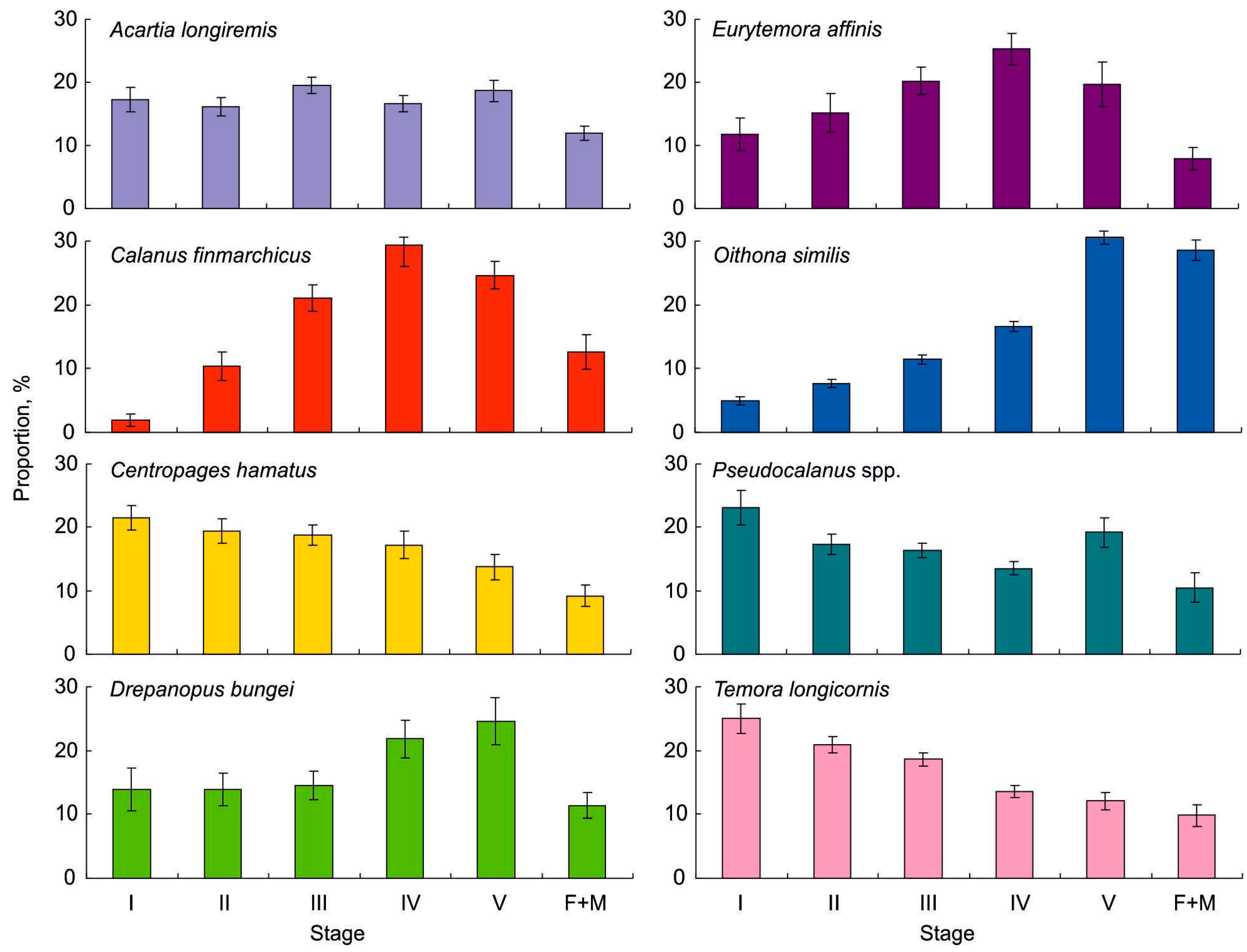
3.2. Copepod Composition, Abundance, Biomass, Diversity, and Population Structure of Common Taxa

We identified 24 taxa of copepods including 16 species of calanoids, 3 species of cyclopoids, 2 species of harpacticoids, and 1 species of poecilostomatoids (Table 3).
The most common taxa were Acartia longiremis, Calanus finmarchicus, Centropages hamatus, Copepoda nauplii, Eurytemora affinis, Oithona similis, Pseudocalanus spp. I-IV, Pseudocalanus minutus V-VI, Pseudocalanus acuspes V-VI, and Temora longicornis. These species occurred at 90% of our stations (Table 3). Species richness was similar at all stations (11–16 taxa or 9–14 species).
The total abundance and biomass of copepod taxa varied over a wide range (Table 3). Spatial patterns of the integrated copepod abundance and biomass are shown in Figure 3a,b.
The maximum abundances were recorded in the central part of the study area, while the highest biomass was found at the southernmost stations. The diversity of the copepod taxa (H’, Shannon index) ranged from 1.86 to 3.01 and tended to be higher in the eastern and northwestern locations (Figure 3c). Evenness (J) demonstrated the same distribution as H’ and varied from 0.52 to 0.84 (Figure 3d).
During the study period, all copepodite stages had similar proportions in the population of Acartia longiremis comprising 16–20% (Figure 4).
The population of Calanus finmarchicus was dominated by CIII–CV copepodite stages, which, together, attained 75% of the total abundance (Figure 4). Copepodites I–III formed the bulk of Centropages hamatus population, accounting for 60% of the total abundance (Figure 4). Older copepodite stages (CIV and CV) and adults comprised more than 50% of the Drepanopus bungei population, whereas CI–CIII specimens also showed high occurrence (Figure 4). The population structure of Eurytemora affinis was characterized by the dominance of copepodites CIII–CIV (20–25%), while adults were relatively rare (Figure 4). The Oithona similis population was mainly represented by CIV–CV copepodites (47%) and adults (29%), whereas young copepodites had low abundance (Figure 4). Younger copepodite stages CI–CIII clearly prevailed in the population of Pseudocalanus minutus/acuspes, comprising 57% of the total abundance, while the proportion of adults was low (Figure 4). A similar population structure was recorded for Temora longicornis, with CI–CIII being the most abundant (65%) (Figure 4).

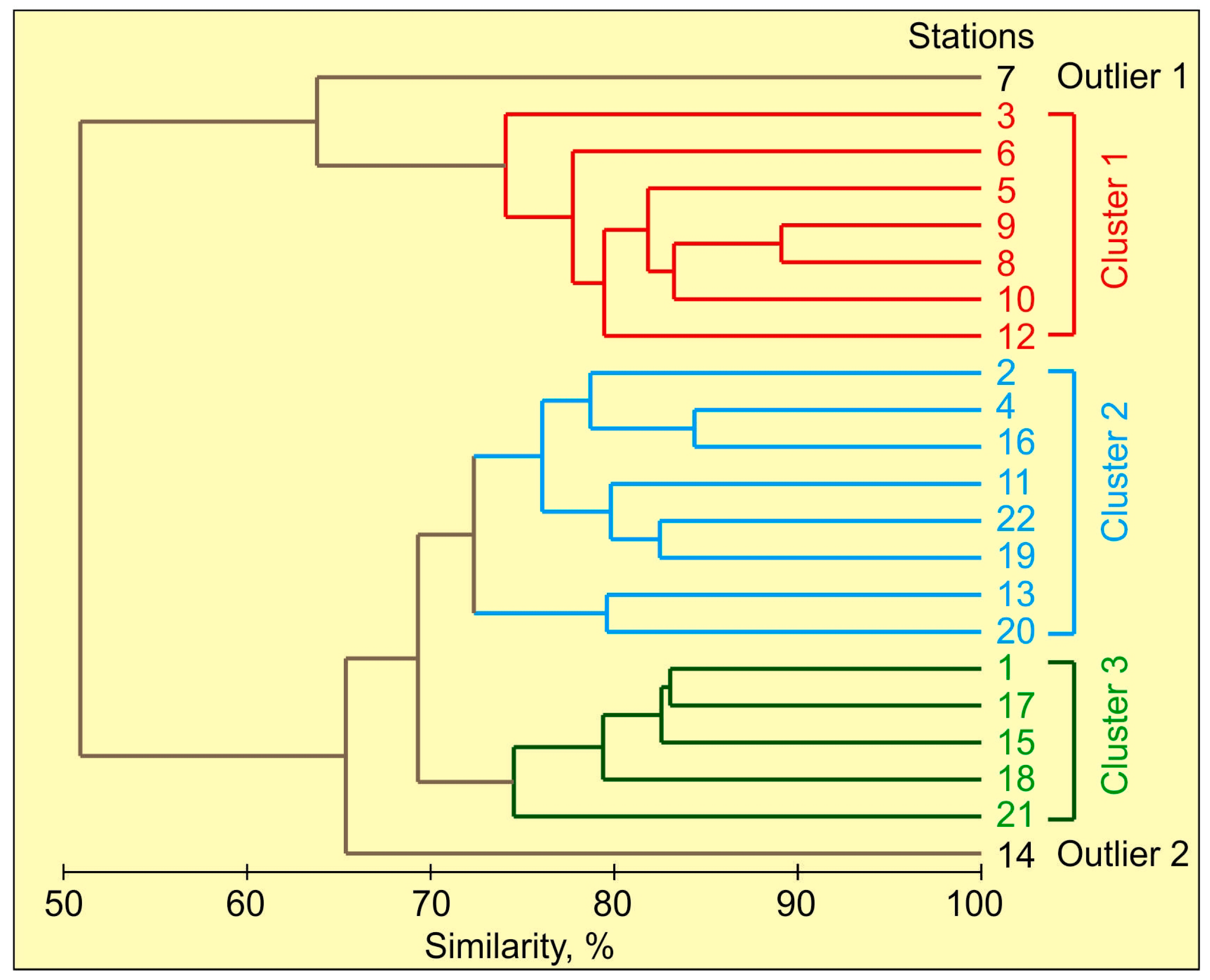
3.3. Copepod Assemblages

The hierarchical cluster analysis of stations resulted in three distinct clusters at a 51% similarity level (Figure 5).
Cluster 1 comprised seven stations located in the northern part of the study area (Figure 1), where both copepod abundance (3892 ± 366 ind. m−3) and biomass (24 ± 4 mgDM m−3) were relatively low. Oithona similis, Copepoda nauplii, and Pseudocalanus inutus/acuspes dominated the copepod assemblage of this cluster in terms of the total abundance (>75%), while Calanus finmarchicus mostly contributed to the total biomass (>40%). SIMPER showed a high degree of similarity between stations in this cluster, with Oithona similis, Copepoda nauplii, and Pseudocalanus spp. being the most important contributing taxa (Table 4).
The mean temperature at stations of Cluster 1 was 6.0 ± 0.5 °C, at least 4 °C cooler than in the rest two groups. The mean salinity (33.22 ± 0.01) was higher at Cluster 1 stations compared to other clusters.
Cluster 2 comprised eight central and southern stations where both abundance (34,725 ± 3342 ind. m−3) and biomass (161 ± 30 mgDM m−3) were high. This group was dominated by Temora longicornis (37% of the total abundance and 56% of the total biomass). High relative densities were registered for Copepoda nauplii (22%) and Oithona similis (12%). These three taxa were the most important contributors to the total similarity between stations in Cluster 2 (Table 4). The minimum copepod evenness (0.63±0.02) and Shannon diversity (2.28 ± 0.08) were found at stations of Cluster 2.
Cluster 3 included five stations: three of them were located in the south-eastern part of the investigated area, and the two others in the south-western and central parts. The copepod assemblage had lower abundance (11,600 ± 1429 ind. m−3) and biomass (46 ± 7 mgDM m−3) compared to Cluster 2, but a higher abundance than in Cluster 1. This group was similar to Cluster 2 and was characterized by high abundances of Temora longicornis (28%), Copepoda nauplii (20%), and Oithona similis (18%). Two species, Temora longicornis and Centropages hamatus, amounted to more than 65% of the total copepod biomass. SIMPER revealed that the similarity between stations in this group was high (Table 4). Moreover, at stations in Cluster 3, we recorded the highest mean chlorophyll a concentration (0.88±0.11 mg m−3) and Shannon diversity (2.67 ± 0.09). Three estuarine species (Jaschnovia tolli, Limnocalanus macrurus, Pseudocalanus major) occurred only at stations of Clusters 2 and 3 while the remaining two brackish-water species (Drepanopus bungei, Eurytemora affinis) were detected throughout the study area but reached maximum densities in the southern part.
Two stations did not group with other clusters and were treated as outliers. Station 7 had low copepod abundance and biomass (1581 ind. m−3 and 35 mgDM m−3, respectively), with Oithona similis and Pseudocalanus spp. being the most numerous (70%). Calanus glacialis accounted for 75% of the total copepod biomass at this station. Station 14 was characterized by the highest copepod abundance (40,146 ind. m−3) and biomass (197 mgDM m−3) within the study area. Copepoda nauplii, Oithona similis, and Pseudocalanus spp. prevailed by abundance (>78%) while Calanus finmarchicus dominated by biomass (53%).
There were significant differences between the station groupings (ANOSIM: global R = 0.9, p = 0.001). A comparison between clusters revealed that abundances of Acartia longiremis, Calanus finmarchicus, Calanus glacialis, Centropages hamatus, Jaschnovia tolli, Microsetella norvegica, Oithona atlantica, Oithona similis, Pseudocalanus minutus/acuspes, Temora longicornis as well as total copepod abundance, Shannon index, mean temperature and salinity were significantly different (ANOVA or Kruskal–Wallis tests, p < 0.05).

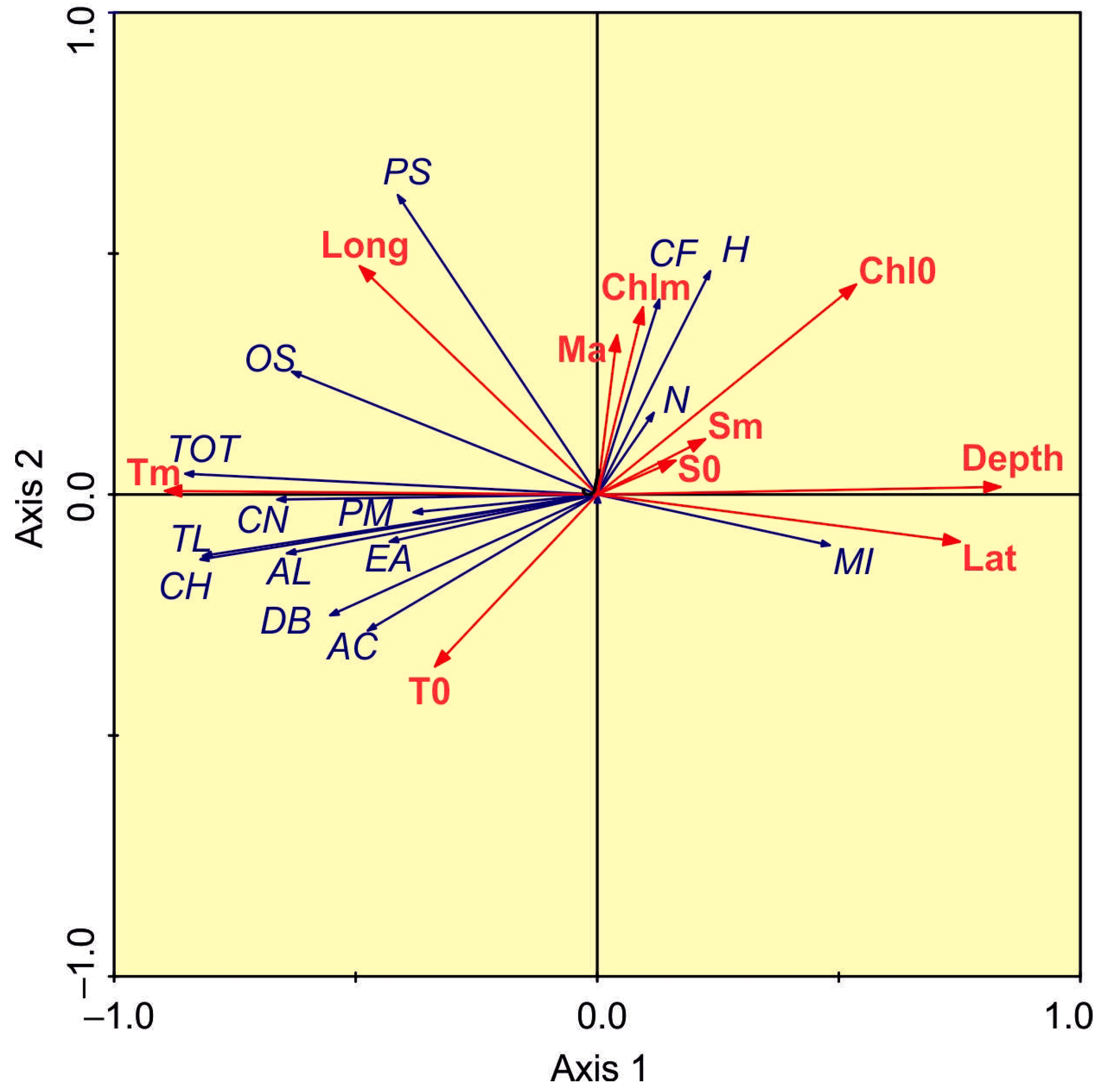
3.4. Environmental Control of Copepod Assemblages

The first two RDA axes explained 93.1% of the total copepod–environmental variability in the south-eastern Barents Sea during the study period (Figure 6).
The first and second RDA axes had eigenvalues of 0.588 and 0.034, respectively, using all environmental variables. For common copepod taxa, the RDA biplot diagram indicated that the first canonical axis, which was the only significant axis (p < 0.001), was positively correlated (p < 0.05) with latitude, surface chlorophyll a concentration, and depth, and negatively correlated with the mean water temperature (Figure 6). The RDA biplot delineated copepod taxa and diversity indices in the study area. The scores of Centropages hamatus, Temora longicornis, Copepoda nauplii, Oithona similis, Acartia spp., Drepanopus bungei, Eurytemora affinis, Pseudocalanus major, Pseudocalanus minutus/acuspes, and the total copepod abundance were grouped together on the biplot diagram, indicating that they were all preferentially located at stations with a higher mean water temperature. Pearson correlation analysis also revealed a positive association between the abundance of these taxa and temperature (Table 5).
The scores of Calanus finmarchicus, Shannon diversity, and species richness were related to the high chlorophyll a concentration (Figure 6), although Pearson correlation analysis revealed a non-significant association between these variables and chlorophyll a (Table 5). The abundance of Microcalanus pusillus tended to increase with sampling depth and latitude (Figure 6), supported by Pearson correlation analysis (Table 5). The Monte-Carlo permutation test showed that the set of environmental variables explained 67% of the total copepod variability; mean water temperature (F = 17.85, p = 0.001, 27%) and surface water temperature (F = 2.76, p = 0.046, 14%) had the largest explanatory power.

4. Discussion

4.1. Environmental Conditions

Coastal waters of the Barents Sea represent an environment with various oceanographic conditions [7,40]. The Pechora Sea Coastal Water is a type of coastal water located in the south-eastern Barents Sea, which is strongly affected by freshened inflow from Pechora Bay [5]. This influence is responsible for the temperature–salinity gradient observed from the inshore to offshore waters. Previous investigations have documented at least three distinct sub-regions that differ from each other in terms of local environmental conditions [7]. The northern waters of the Pechora Sea are similar to the open sea waters, characterized by high salinity and low temperature. They represent a mixing of the White Sea Water and the Kara Sea Water (Litke Current) [6]. The water column is clearly stratified in the deep northern parts of the Pechora Sea. The central part of the Pechora Sea is influenced by the Kolguyev–Pechora Current, with an Atlantic origin [68]. The southern part of the Pechora Sea is strongly affected by freshwater run-off from the Pechora River, which leads to reduced salinity and a higher water temperature [7]. A frontal zone separates the coastal freshening zone and the inshore regions [40]. Additionally, there is a very complicated system of local currents and eddies that significantly affect the spatial patterns of temperature and salinity in the Pechora Sea [6]. Our study area included regions that are less impacted by freshwater discharge than areas in the Pechora River Delta and adjacent waters. However, a spatial temperature/salinity gradient was found from the south-eastern to the north-western sampling stations.
Comparisons with multi-year summer temperatures recorded in the south-eastern Barents Sea (1952–2001) [69] revealed a higher water temperature in the summer of 2012, suggesting warm conditions during our study. This observation is in line with recent findings showing climatic changes in the Arctic in recent decades [70,71,72]. The warming of the Barents Sea is a well-documented phenomenon that can directly affect marine biota, including plankton assemblages [36,42,73].
We found low chlorophyll a concentration within the whole study area, which suggests a post-bloom period in the Pechora Sea in July–August. Previous investigations have shown that the bloom period in the southern and south-eastern Barents occurs in April, with Thalassiosira, Chaetoceros, Navicula, and Pleurosigma being the most abundant phytoplankton [1,8,9,10,74]. There may also be a late-spring peak in microalgae in this region in June [9]. Therefore, we may assume reduced food availability for copepods relative to the main phytoplankton growth period.

4.2. Copepod Composition, Abundance, Biomass, Diversity, and Population Structure of Common Taxa

In the present material, the copepod composition was in accordance with earlier mesozooplankton investigations in the Pechora Sea [29,43]. The most frequent taxa in our study were also noted among the most abundant copepods in previous studies in different coastal regions of the Barents Sea and adjacent waters [12,30,32,33,34,35,37]. The presence of some brackish and estuarine taxa was registered in our study. Jaschnovia tolli, Limnocalanus macrurus, and Pseudocalanus major were found in the southern part of the study area, which had less saline water. Drepanopus bungei and Eurytemora affinis were also recorded in the southern regions but their abundance tended to be higher in freshened waters, showing their preference for estuarine conditions. These five taxa represent typical brackish neritic species inhabiting Arctic coastal regions affected by freshwater run-off [22,46]. They were recorded in the Kara, Laptev, and Beaufort Seas [75,76,77,78,79]. Therefore, the copepod fauna in our study represented a mix of typical marine taxa and estuarine species. This explains the higher species richness and Shannon diversity of copepod communities in comparison to other coastal regions of the Barents Sea without a strong freshwater influence [30,32,33,34,35,37,38]. Maximal values of diversity and evenness were found in the south-eastern and the north-western stations, where the environmental conditions were most diverse. Frontal zones are considered to be the regions with the richest marine biota [1], and our study confirms this general pattern.
Zooplankton sampling methods and net mesh size were found to be significant factors affecting abundance estimates and species composition of the catch. In our study, the total copepod abundance ranged from 69 to 935·103 ind. m−2 (from 1581 to 47,381 ind. m−3), and was higher than in previous studies [29,43]. The mean density of Copepoda was 95–101 103 ind. m−2 in early–mid-July 2001 (168 μm mesh net) [29] and 6617 ind m−3 in mid-July 2014 (100 μm mesh net) [43]. Moreover, our estimations were lower than those obtained in early September 2016 (19,166 ind. m−3; 168 μm mesh net) [43] in the eastern Pechora Sea. Despite the coarser net used in the present study, our values were significantly greater than those previously recorded. Usov et al. [43] used a 100 μm net to collect mesozooplankton, whereas we caught copepods with a 168 μm net that, in fact, may undersample a small-copepods fraction, leading to underestimations of the total copepod density. Additionally, the differences in copepod abundance might also be related to seasonal and spatial variations during the mentioned investigations. Copepod biomass in our study was also higher than the previously recorded values [29], suggesting higher copepod productivity in the summer of 2012. Climatic differences might also have an influence on the total copepod abundance and biomass during different study periods in the Pechora Sea.
We revealed clear differences in the population structure of common taxa during the study period. In general, populations of small copepod species (Temora, Acartia, and Centropages) tended to be dominated by young stages (copepodites I–III), suggesting their reproduction. The only exception was Oithona similis, but the lower abundance of their earliest copepodites might be related to net undersampling. Populations of Drepanopus bungei and Eurytemora affinis were characterized by a rather homogenous population structure, also suggesting their spawning in the Pechora Sea. Small and opportunistic taxa have been found to be omnivorous and can utilize detritus, suspended organic matter, and bacterioplankton for growth and spawning [80,81]. Herbivorous taxa strongly depend on phytoplankton bloom, and their spawning coincides with peaks in microalgae or occur somewhat later [11,82]. We recorded the dominance of older copepodite stages in the populations of Calanus finmarchicus and Pseudocalanus minutus/acuspes, and this could be explained by phytoplankton’s succession in the Pechora Sea, i.e., the blooming in April or June. Earlier studies have reported that the life-cycle of Calanus finmarchicus is controlled by phytoplankton dynamics in many Arctic regions [12,82]. The reproduction of Pseudocalanus in Arctic and Atlantic waters is prolonged, but spawning events in this species are also linked to phytoplankton dynamics [83,84].

4.3. Copepod Assemblages

Our study revealed three distinct copepod assemblages in the Pechora Sea, corroborating our main hypothesis. There was a spatial trend of copepod assemblages from the south-eastern to the north-western regions. Overall, high similarity was observed in the copepod community composition. The main differences between the assemblages delineated with the cluster analysis were related to the total abundance, biomass, proportions of common copepod taxa, and the presence of estuarine and brackish species. Many of the copepod taxa occurred at most sampling stations.
The first cluster may be defined as a true marine community with a high abundance of Oithona similis, Copepoda nauplii, and Pseudocalanus inutus/acuspes, the presence of Calanus finmarchicus, and low proportions of neritic species. This assemblage is typical for other coastal waters of the southern Barents Sea and is mainly associated with waters of Atlantic origin [32,33,34,35,37,38]. The presence of Calanus glacialis, a true Arctic species, possibly reflected the influence of cold waters from the Kara Sea. The cooler temperatures and higher salinities that persisted at stations of Cluster 1 confirm the greater influence of oceanic water during the study period.
The second cluster represented an intermediate assemblage, including marine, neritic, and brackish water species, and their total abundance and biomass were highest at stations of this cluster. The high copepod concentrations might be associated with local eddies or a frontal zone separating oceanic and inshore waters in the Pechora Sea [6,7,40]. Patchiness in zooplankton distribution is a well-documented phenomenon in marine environments worldwide [11,23,85]. Several studies have shown the enhanced productivity of plankton in regions where there is a mixing of different water masses [85,86]. For example, the Marginal Ice Zone and Polar Front waters are considered to be one of the most productive and diverse areas in the Barents Sea [1,87]. Similar patterns were noted in Arctic estuarine regions [77,78,87,88]. The high diversity in plankton distributions and large copepod stocks in the investigated area reflected substantial fluctuations in physical conditions. A wide range of habitual niches was available to the copepods at Cluster 2 stations, which was favorable for their successful growth and development.
The third cluster was characterized by the highest abundance of estuarine taxa (Jaschnovia tolli, Limnocalanus macrurus, and Pseudocalanus major), suggesting a strong impact of freshwater discharge on the copepod assemblage. The lowest salinity and highest water temperature recorded here support this conclusion. The local community was the most diverse among the three assemblages. This result is expected because marine, neritic, and estuarine taxa occurred at stations of Cluster 3. Marine taxa seem likely to originate from more northern locations, while estuarine and brackish species might have been advected from the southern Pechora Sea.
Previous investigations have revealed a pronounced separation of mesozooplankton assemblages in the Pechora Sea along the environmental gradients [29,43]. For instance, three groups of stations, based on zooplankton abundance, were detected in the south-eastern Barents Sea. These assemblages (Marine, Intermediate, and Brackish) differed significantly in composition, abundance, and biomass. Three copepod taxa, Calanus finmarchicus, Pseudocalanus species, and Limnocalanus macrurus, made the highest contribution to the total mesozooplankton biomass within each single cluster [29]. A similar result was reported in the Kara Sea, where five zooplankton groups were present from the inshore freshened waters to the open sea area [76]. Zooplankton assemblages in the Laptev Sea were found to differ in terms of composition and abundance depending on the environmental conditions [75,77]. In the Beaufort Sea, seven faunal groupings of mesozooplankton were revealed, in association with temperature and salinity gradients [79]. Thus, the clear spatial differences in mesozooplankton/copepod assemblages within the environmental gradients should be considered a common feature in Arctic marine coastal regions affected by freshwater discharge. Compared with our previous zooplankton investigation in the Pechora Sea [29], we revealed a lower proportion of brackish water species and the absence of freshwater copepods in summer 2012. This discrepancy can be explained by differences in the location of sampling sites; namely, in 2001, we studied inshore waters of the Pechora Sea with a higher freshwater impact [29], while in 2012, our study focused on the offshore regions that were more affected by oceanic waters.

4.4. Environmental Control of Copepod Assemblages

Fine-scale variations in the environmental parameters may have a significant impact on mesozooplankton assemblages in Arctic waters [36,37,58]. Water mass properties, especially temperature and salinity, are primary factors affecting spatial patterns in the plankton distribution in the Barents Sea [37,39]. We revealed that environmental variables explained more than 67% of the copepod variability in the Pechora Sea. Three factors (mean and surface water temperature, and depth) were the most important drivers of copepod abundance during our study. Water temperature has been documented to be among the most important properties influencing plankton animals in many Arctic regions, controlling their growth and development [11,23]. This factor reflects the distribution of different water masses at spatial and temporal scales [3]. Two main types of zooplankton assemblages in the Barents Sea (Atlantic and Arctic) were mainly delineated based on the temperature of water masses [5]. Cold-water taxa dominate zooplankton assemblages in Arctic Water while boreal species are most abundant in Atlantic Water [12,42]. Coastal Water has a specific feature, varying water temperature, leading to separated mesozooplankton assemblages in accordance with temperature changes [32,34,35,38]. Our study revealed a clear spatial trend in water temperature, and the copepod assemblages differed in association with these temperature variations. The abundances of common small neritic taxa negatively correlated with the sampling depth. This result is expected and may be explained by their preference for shallow water locations with higher water temperatures, as reported for many small neritic copepods inhabiting coastal waters of the Barents Sea [22,32,33,35,38].
The RDA and Pearson correlation analysis found a non-significant impact of salinity on the copepod assemblages, and this is in contradiction with previous findings on the mesozooplankton of the Pechora Sea [29,43]. Salinity has also been reported to be one of the most important factors affecting mesozooplankton communities in Arctic marine estuaries [76,77,79]. In the northern White Sea, a region bordering the south-eastern Barents Sea, mean mesozooplankton abundance and biomass were positively correlated with water salinity. The high variability and low salinity values restricted the occurrence of marine zooplankton in the northern White Sea [89]. In our study, the mean salinity was 30–34 psu. We may suppose that this salinity gradient was too low to have a strong influence on the copepod distribution. Previously, we documented a clear association between salinity and mesozooplankton in the Pechora Sea [29] when the salinity gradient was >20 psu (13.50–34.98). Only one species (Pseudocalanus major) in the present study demonstrated a significant negative correlation with salinity, indicating their clear preference for brackish waters, consistent with their biology and ecology [22].
Both oceanography and biota have been reported to be strongly affected by tidal currents in many coastal regions worldwide [11,86]. The coastal waters in the Pechora Sea have been documented to be strongly influenced by high tides and tidal currents, with the strongest impact occurring in the inshore regions (Pechora Bay and adjacent waters) [6], while tidal effects become weaker in more offshore areas, as in our case. We found that some neritic brackish taxa (Drepanopus bungei and Eurytemora affinis) occurred throughout the entire study area. Additionally, we revealed patchiness in the copepod distribution. These findings could be explained by the local circulation in the offshore regions of the Pechora Sea, advection of freshwater masses, and tidal currents from the inshore regions. Strong hydrological stratification may also have an impact on the copepod assemblages. A similar result was recorded for macrozooplankton in the Pechora Sea [40]. Therefore, our data indicate that the complicated circulation pattern and local hydrographic conditions seem to be responsible for the heterogeneity in the copepod distribution in the Pechora Sea.
The availability of food resources is considered an important driver of mesozooplankton in the Arctic ecosystems [12,24]. Although the surface chlorophyll a concentration explained 8% of the total copepod variability, we did not detect significant correlations between copepod density and this parameter. Some investigations reported similar results [40,90,91], while other studies have shown a direct correlation between zooplankton density and phytoplankton concentration [35,88,92,93,94,95]. We may also propose that other food sources could affect copepod assemblages in the Pechora Sea. Considering the dominance of omnivorous taxa, microzooplankton, bacterioplankton, detritus, and particulate organic carbon would be important food sources for the copepods. Our hypothesis is supported by several studies that suggest that small and opportunistic taxa are able to ingest ciliates, organic macroaggregates, and marine bacteria [80,96].
Predatory pressure may also be an important factor controlling the density of zooplankton communities [42,97]. Our analysis did not indicate significant correlations between copepod abundance and the total number of macrozooplankton, suggesting a low influence of large carnivorous plankters on the copepod assemblages. This may be explained by the low abundance of macrozooplankton during the study period. Additionally, we did not consider ichthyioplankton and larval fish, which might be important copepod consumers in the Pechora Sea.

5. Conclusions

The Arctic is a complex ecosystem and the role of plankton in this ecosystem is largely unexplored, particularly in the estuarine regions. This study provides a baseline description of copepod assemblages in the south-eastern Barents Sea, an area strongly affected by freshwater discharge from the Pechora River. We revealed changes in the copepod composition, abundance, biomass, and diversity in relation to variations in some important abiotic and biotic factors. Our report may be applied to assessments of ecosystem health and the possible responses of local biota to environmental influence. Recent global climatic changes have become obvious as warming in the Arctic leads to shifts in marine ecosystems. To evaluate the climatic impacts on the pelagic ecosystems, baseline investigations are needed. Our data may also be useful to reveal the possible ecosystem fluctuations related to intense human activity in the Pechora Sea, namely, gas–oil development and exploitation, shipping, and local fishing.

Author Contributions

Conceptualization, V.G.D. and A.G.D.; methodology, V.G.D.; software, V.G.D.; validation, A.G.D.; formal analysis, V.G.D. and A.G.D.; investigation, V.G.D.; resources, V.G.D.; data curation, A.G.D.; writing—original draft preparation, V.G.D. and A.G.D.; writing—review and editing, V.G.D. and A.G.D.; visualization, V.G.D. and A.G.D.; supervision, A.G.D.; project administration, A.G.D. All authors have read and agreed to the published version of the manuscript.

Funding

This study was funded by the Ministry of Science and Higher Education of the Russian Federation.

Institutional Review Board Statement

Not applicable.

Informed Consent Statement

Not applicable.

Data Availability Statement

The data are available on request from the corresponding author.

Acknowledgments

We are grateful to the crew of the R/V Dalnie Zelentsy and the on-board scientists for their support during sampling. Thanks are due to K.A. Bobrov for hydrological data and V.V. Vodopyanova for chlorophyll a analysis. Thanks to the three anonymous reviewers for their criticism of the manuscript.

Conflicts of Interest

The authors declare no conflict of interest.

References

  1. Wassmann, P.; Reigstad, M.; Haug, T.; Rudels, B.; Carroll, M.L.; Hop, H.; Gabrielsen, G.W.; Falk-Petersen, S.; Denisenko, S.G.; Arashkevich, E.; et al. Food webs and carbon flux in the Barents Sea. Prog. Oceanogr. 2006, 71, 232–287. [Google Scholar] [CrossRef]
  2. Dvoretsky, V.G.; Dvoretsky, A.G. Ecology and Distribution of Red King Crab Larvae in the Barents Sea: A Review. Water 2022, 14, 2328. [Google Scholar] [CrossRef]
  3. Ingvaldsen, R.; Loeng, H. Physical Oceanography. In Ecosystem Barents Sea; Sakshaug, E., Johnsen, G., Kovacs, K., Eds.; Tapir Academic Press: Trondheim, Norway, 2009; pp. 33–64. [Google Scholar]
  4. Loeng, H. Features of the physical oceanographic conditions in the central parts of the Barents Sea. Polar Res. 1991, 10, 5–18. [Google Scholar] [CrossRef] [Green Version]
  5. Ozhigin, V.K.; Ingvaldsen, R.B.; Loeng, H.; Boitsov, V.; Karsakov, A. Introduction to the Barents Sea. In The Barents Sea ecosystem: Russian-Norwegian cooperation in science and management; Jakobsen, T., Ozhigin, V., Eds.; Tapir Academic Press: Trondheim, Norway, 2011; pp. 315–328. [Google Scholar]
  6. Nikiforov, S.L.; Dunaev, N.N.; Politova, N.V. Modern environmental conditions of the Pechora Sea (climate, currents, waves, ice regime, tides, river runoff, and geological structure). Ber. Polarforsch. 2005, 501, 7–38. [Google Scholar]
  7. Sukhotin, A.; Denisenko, S.; Galaktionov, K. Pechora Sea ecosystems: Current state and future challenges. Polar Biol. 2019, 42, 1631–1645. [Google Scholar] [CrossRef]
  8. Sakshaug, E.; Johnsen, G.; Kristiansen, S.; von Quillfeldt, C.; Rey, F.; Slagstad, D.; Thingstad, F. Phytoplankton and primary production. In Ecosystem Barents Sea; Sakshaug, E., Johnsen, G., Kovacs, K., Eds.; Tapir Academic Press: Trondheim, Norway, 2009. [Google Scholar]
  9. Makarevich, P.; Druzhkova, E.; Larionov, V. Primary producers of the Barents Sea. In Diversity of Ecosystems; Mahamane, A., Ed.; In Tech: Rijeka, Croatia, 2012; pp. 367–392. [Google Scholar]
  10. Makarevich, P.R.; Vodopianova, V.V.; Bulavina, A.S.; Vashchenko, P.S.; Ishkulova, T.G. Features of the distribution of chlorophyll-a concentration along the western coast of the Novaya Zemlya archipelago in spring. Water 2021, 13, 3648. [Google Scholar] [CrossRef]
  11. Raymont, J.E.G. Plankton and Productivity in the Ocean, 2. Zooplankton, 2nd ed.; Pergamon Press: Oxford, UK, 1983. [Google Scholar]
  12. Eiane, K.; Tande, K.S. Meso and macrozooplankton. In Ecosystem Barents Sea; Sakshaug, E., Johnsen, G., Kovacs, K., Eds.; Tapir Academic Press: Trondheim, Norway, 2009; pp. 209–234. [Google Scholar]
  13. Dvoretsky, A.G.; Dvoretsky, V.G. Commercial fish and shellfish in the Barents Sea: Have introduced crab species affected the population trajectories of commercial fish? Rev. Fish Biol. Fisheries 2015, 25, 297–322. [Google Scholar] [CrossRef]
  14. Dvoretsky, A.G.; Dvoretsky, V.G. Red king crab (Paralithodes camtschaticus) fisheries in Russian waters: Historical review and present status. Rev. Fish Biol. Fish. 2017, 28, 331–353. [Google Scholar] [CrossRef]
  15. Olsen, E.; Aanes, S.; Mehl, S.; Holst, J.C.; Aglen, A.; Gjøsæter, H. Cod, haddock, saithe, herring, and capelin in the Barents Sea and adjacent waters: A review of the biological value of the area. ICES J. Mar. Sci. 2009, 67, 87–101. [Google Scholar] [CrossRef]
  16. Hop, H.; Gjøsæter, H. Polar cod (Boreogadus saida) and capelin (Mallotus villosus) as key species in marine food webs of the Arctic and the Barents Sea. Mar. Biol. Res. 2013, 9, 878–894. [Google Scholar] [CrossRef]
  17. Semushin, A.V.; Novoselov, A.P.; Sherstkov, V.S.; Levitsky, A.L.; Novikova, Y.V. Long-term changes in the ichthyofauna of the Pechora Sea in response to ocean warming. Polar Biol. 2019, 42, 1739–1751. [Google Scholar] [CrossRef]
  18. Shiskin, A.N. Ecological Atlas. Barents Sea; NIR Moscow: Moscow Russia, 2020. (In Russian) [Google Scholar]
  19. Margiotta, F.; Balestra, C.; Buondonno, A.; Casotti, R.; D’Ambra, I.; Di Capua, I.; Gallia, R.; Mazzocchi, M.G.; Merquiol, L.; Pepi, M.; et al. Do plankton reflect the environmental quality status? The case of a post-industrial Mediterranean Bay. Mar. Environ. Res. 2020, 160, 104980. [Google Scholar] [CrossRef]
  20. Dvoretsky, A.G.; Dvoretsky, V.G. Effects of environmental factors on the abundance, biomass, and individual weight of juvenile red king crabs in the Barents Sea. Front. Mar. Sci. 2020, 7, 726. [Google Scholar] [CrossRef]
  21. McGinty, N.; Barton, A.D.; Record, N.R.; Finkel, Z.V.; Johns, D.G.; Stock, C.A.; Irwin, A.J. Anthropogenic climate change impacts on copepod trait biogeography. Glob. Chang. Biol. 2020, 27, 1431–1442. [Google Scholar] [CrossRef]
  22. Brodsky, K.A. Calanoida of the Far Eastern Seas and Polar Basin of the USSR; Israel Program Scientific Translation: Jerusalem, Israel, 1967. [Google Scholar]
  23. Castellani, C.; Edwards, M. Marine Plankton: A Practical Guide to Ecology, Methodology, and Taxonomy; Oxford University Press: Oxford, UK, 2017. [Google Scholar]
  24. Vadstein, O. Interactions in the planktonic food web. In Ecosystem Barents Sea; Sakshaug, E., Johnsen, G., Kovacs, K., Eds.; Tapir Academic Press: Trondheim, Norway, 2009; pp. 251–266. [Google Scholar]
  25. Box, J.E.; Colgan, W.T.; Christensen, T.R.; Schmidt, N.M.; Lund, M.; Parmentier, F.-J.W.; Brown, R.; Bhatt, U.S.; Euskirchen, E.S.; Romanovsky, V.E.; et al. Key indicators of Arctic climate change: 1971–2017. Environ. Res. Lett. 2019, 14, 045010. [Google Scholar] [CrossRef]
  26. Long, Y.; Noman, A.; Chen, D.; Wang, S.; Yu, H.; Chen, H.; Wang, M.; Sun, J. Western Pacific Zooplankton Community along Latitudinal and Equatorial Transects in Autumn 2017 (Northern Hemisphere). Diversity 2021, 13, 58. [Google Scholar] [CrossRef]
  27. Richardson, A.J. In hot water: Zooplankton and climate change. ICES J. Mar. Sci. 2008, 65, 279–295. [Google Scholar] [CrossRef] [Green Version]
  28. Deschutter, Y.; Everaert, G.; De Schamphelaere, K.; De Troch, M. Relative contribution of multiple stressors on copepod density and diversity dynamics in the Belgian part of the North Sea. Mar. Pollut. Bull. 2017, 125, 350–359. [Google Scholar] [CrossRef] [PubMed]
  29. Dvoretsky, V.G.; Dvoretsky, A.G. Summer mesozooplankton structure in the Pechora Sea (south-eastern Barents Sea). Estuarine Coast. Shelf Sci. 2009, 84, 11–20. [Google Scholar] [CrossRef]
  30. Dvoretsky, V.G.; Dvoretsky, A.G. Summer mesozooplankton distribution near Novaya Zemlya (eastern Barents Sea). Polar Biol. 2009, 32, 719–731. [Google Scholar] [CrossRef]
  31. Dvoretsky, V.; Dvoretsky, A. Spatial variations in reproductive characteristics of the small copepod Oithona similis in the Barents Sea. Mar. Ecol. Prog. Ser. 2009, 386, 133–146. [Google Scholar] [CrossRef]
  32. Dvoretsky, V.G.; Dvoretsky, A.G. Mesozooplankton structure in Dolgaya Bay (Barents Sea). Polar Biol. 2009, 33, 703–708. [Google Scholar] [CrossRef]
  33. Dvoretsky, V.G.; Dvoretsky, A.G. Checklist of fauna found in zooplankton samples from the Barents Sea. Polar Biol. 2010, 33, 991–1005. [Google Scholar] [CrossRef]
  34. Dvoretsky, V.G.; Dvoretsky, A.G. Copepod communities off Franz Josef Land (northern Barents Sea) in late summer of 2006 and 2007. Polar Biol. 2011, 34, 1231–1238. [Google Scholar] [CrossRef]
  35. Dvoretsky, V.G.; Dvoretsky, A.G. Estimated copepod production rate and structure of mesozooplankton communities in the coastal Barents Sea during summer–autumn 2007. Polar Biol. 2012, 35, 1321–1342. [Google Scholar] [CrossRef]
  36. Dvoretsky, V.G.; Dvoretsky, A.G. Epiplankton in the Barents sea: Summer variations of mesozooplankton biomass, community structure and diversity. Cont. Shelf Res. 2012, 52, 1–11. [Google Scholar] [CrossRef]
  37. Dvoretsky, V.G.; Dvoretsky, A.G. Structure of mesozooplankton community in the Barents Sea and adjacent waters in August 2009. J. Nat. Hist. 2013, 47, 2095–2114. [Google Scholar] [CrossRef]
  38. Dvoretsky, V.G.; Dvoretsky, A.G. Summer mesozooplankton community of Moller Bay (Novaya Zemlya Archipelago, Barents Sea). Oceanologia 2013, 55, 205–218. [Google Scholar] [CrossRef] [Green Version]
  39. Dvoretsky, V.G.; Dvoretsky, A.G. Mesozooplankton in the Kola Transect (Barents Sea): Autumn and winter structure. J. Sea Res. 2018, 142, 125–131. [Google Scholar] [CrossRef]
  40. Dvoretsky, V.G.; Dvoretsky, A.G. Summer-fall macrozooplankton assemblages in a large Arctic estuarine zone (south-eastern Barents Sea): Environmental drivers of spatial distribution. Mar. Environ. Res. 2022, 173. [Google Scholar] [CrossRef]
  41. Dvoretsky, V.G.; Dvoretsky, A.G. Coastal Mesozooplankton Assemblages during Spring Bloom in the Eastern Barents Sea. Biology 2022, 11, 204. [Google Scholar] [CrossRef]
  42. Dalpadado, P.; Arrigo, K.R.; van Dijken, G.L. Skjoldal, H.R.; Bagøien, E, Dolgov A.V.; Prokopchuk, I.P.; Sperfeld, E. Climate effects on temporal and spatial dynamics of phytoplankton and zooplankton in the Barents Sea. Progr. Oceanogr. 2020, 182, 102320. [Google Scholar]
  43. Usov, N.; Khaitov, V.; Smirnov, V.; Sukhotin, A. Spatial and temporal variation of hydrological characteristics and zooplankton community composition influenced by freshwater runoff in the shallow Pechora Sea. Polar Biol. 2018, 42, 1647–1665. [Google Scholar] [CrossRef]
  44. Lorenzen, C.J. Determination of chlorophyll and pheo-pigments: Spectrophotometric equations. Limnol. Oceanogr. 1967, 12, 343–346. [Google Scholar] [CrossRef]
  45. Parsons, T.R.; Maita, Y.; Lalli, C.M. A manual of chemical & biological methods for seawater analysis. Mar. Pollut. Bull. 1984, 1, 101–112. [Google Scholar]
  46. Jaschnov, V.A. Order Copepoda. In Guide to the Fauna and Flora of Northern Seas of the USSR; Gaevskaya, N.S., Ed.; Soviet Nauka Press: Moscow, USSR, 1948; pp. 183–215. (In Russian) [Google Scholar]
  47. Shuvalov, V.S. Copepod Cyclopoids of the Family Oithonidae of the World Ocean; Nauka Press: Leningrad, USSR, 1980. (In Russian) [Google Scholar]
  48. Madsen, S.D.; Nielsen, T.G.; Hansen, B.W. Annual population development and production by Calanus finmarchicus, C. glacialis and C. hyperboreus in Disko Bay, western Greenland. Mar. Biol. 2001, 139, 75–93. [Google Scholar]
  49. Dvoretsky, V.G. Distribution of Calanus species off Franz Josef Land (Arctic Barents Sea). Polar Sci. 2011, 5, 361–373. [Google Scholar] [CrossRef] [Green Version]
  50. Choquet, M.; Kosobokova, K.; Kwaśniewski, S.; Hatlebakk, M.; Dhanasiri, A.K.S.; Melle, W.; Daase, M.; Svensen, C.; Søreide, J.E.; Hoarau, G. Can morphology reliably distinguish between the copepods Calanus finmarchicus and C. glacialis, or is DNA the only way? Limnol. Oceanogr. Methods 2018, 16, 237–252. [Google Scholar] [CrossRef] [Green Version]
  51. Frost, B.W. A taxonomy of the marine calanoid copepod genus Pseudocalanus. Can. J. Zool. 1989, 67, 525–551. [Google Scholar] [CrossRef]
  52. Berggreen, U.; Hansen, B.; Kiørboe, T. Food size spectra, ingestion and growth of the copepod Acartia tonsa during development: Implications for determination of copepod production. Mar. Biol. 1988, 99, 341–352. [Google Scholar] [CrossRef]
  53. Ashjian, C.J.; Campbell, R.G.; Welch, H.E.; Butler, M.; Keuren, D.V. Annual cycle in abundance, distribution, and size in relation to hydrography of important copepod species in the western Arctic Ocean. Deep-Sea Res. I 2003, 50, 1235–1261. [Google Scholar] [CrossRef]
  54. Klein Breteler, W.C.M.; Fransz, H.G.; Gonzales, S.R. Growth and development of four calanoid copepod species under experimental and natural conditions. Neth. J. Sea Res. 1982, 16, 195–207. [Google Scholar] [CrossRef]
  55. Sabatini, M.; Kiørboe, T. Egg production, growth and development of the cyclopoid copepod Oithona similis. J. Plankton Res. 1994, 16, 1329–1351. [Google Scholar] [CrossRef] [Green Version]
  56. Satapoomin, S. Carbon content of some common tropical Andaman Sea copepods. J. Plankton Res. 1999, 21, 2117–2123. [Google Scholar] [CrossRef]
  57. Middlebrook, K.; Roff, J.C. Comparison of Methods for Estimating Annual Productivity of the Copepods Acartia hudsonica and Eurytemora herdmani in Passamaquoddy Bay, New Brunswick. Can. J. Fish. Aquat. Sci. 1986, 43, 656–664. [Google Scholar] [CrossRef]
  58. Richter, C. Regional and seasonal variability in the vertical distribution of mesozooplankton in the Greenland Sea. Ber. Zur Polarforsch. 1994. [Google Scholar] [CrossRef]
  59. Kankaala, P.; Johansson, S. The influence of individual variation on length-biomass regressions in three crustacean zooplankton species. J. Plankton Res. 1986, 8, 1027–1038. [Google Scholar] [CrossRef]
  60. Liu, H.; Hopcroft, R.R. Growth and development of Metridia pacifica (Copepoda: Calanoida) in the northern Gulf of Alaska. J. Plankton Res. 2006, 28, 769–781. [Google Scholar] [CrossRef] [Green Version]
  61. Webber, M.K.; Roff, J.C. Annual biomass and production of the oceanic copepod community off Discovery Bay, Jamaica. Mar. Biol. 1995, 123, 481–495. [Google Scholar] [CrossRef]
  62. Postel, L.; Fock, H.; Hagen, W. Biomass and abundance. In ICES Zooplankton Methodology Manual; Harris, R., Wiebe, P., Lenz, J., Skjoldal, H.R., Huntley, M., Eds.; Academic Press: London, UK, 2000; pp. 83–192. [Google Scholar]
  63. Field, J.; Clarke, K.; Warwick, R. A Practical Strategy for Analysing Multispecies Distribution Patterns. Mar. Ecol. Prog. Ser. 1982, 8, 37–52. [Google Scholar] [CrossRef]
  64. Shannon, C.B.; Weaver, W. The Mathematical Theory of Communication; University of Illinois Press: Urbana, USA, 1963. [Google Scholar]
  65. Pielou, E.C. The measurement of diversity in different types of biological collections. J. Theor. Biol. 1966, 13, 131–144. [Google Scholar] [CrossRef]
  66. ter Braak, C.J.F.; Verdonschot, P.F.M. Canonical correspondence analysis and related multivariate methods in aquatic ecology. Aquat. Sci. 1995, 57, 255–289. [Google Scholar] [CrossRef]
  67. ter Braak, C.J.F.; Smilauer, P. CANOCO Reference Manualand CanoDraw for Windows User’s Guide: Software for Canonical Community Ordination (version 4.5); Microcomputer Power: Ithaca, NY, USA, 2002. [Google Scholar]
  68. Pfirman, S.; Kögeler, J.W.; Anselme, B. Coastal environments of the Western Kara and Eastern Barents Seas. Deep Sea Res. 1995, 42, 1391–1412. [Google Scholar] [CrossRef]
  69. Matishov, G.G.; Zuyev, A.N.; A Golubev, V.; Adrov, N.M.; Timofeev, S.F.; Karamusko, O.; Pavlova, L.; Fadyakin, O.; Buzan, A.; Braunstein, A.; et al. Original source of the “Climatic Atlas of the Arctic Seas 2004: Part I. Database of the Barents, Kara, Laptev, and White Seas-Oceanography and Marine Biology”. Available online: https://elibrary.ru/item.asp?id=23200679 (accessed on 29 December 2022).
  70. Drinkwater, K.; Loeng, H.; Titov, O.V.; Boitsov, V.D. Global warming and climate change. In The Barents Sea. Ecosystem, Resources, Management; Jakobsen, T., Ozhigin, V.K., Eds.; Tapir Academic Publishers: Trondheim, Norway, 2011; pp. 777–807. [Google Scholar]
  71. Møller, E.F.; Nielsen, T.G. Borealization of Arctic zooplankton – smaller and less fat zooplankton species in Disko Bay. Western Greenland. Limnol. Oceanogr. 2020, 65, 1175–1188. [Google Scholar] [CrossRef]
  72. Evseeva, O.Y.; Ishkulova, T.G.; Dvoretsky, A.G. Environmental Drivers of an Intertidal Bryozoan Community in the Barents Sea: A Case Study. Animals 2022, 12, 552. [Google Scholar] [CrossRef] [PubMed]
  73. Dvoretsky, A.G.; Dvoretsky, V.G. Inter-annual dynamics of the Barents Sea red king crab (Paralithodes camtschaticus) stock indices in relation to environmental factors. Polar Sci. 2016, 10, 541–552. [Google Scholar] [CrossRef]
  74. Makarevich, P.R.; Vodopianova, V.V.; Bulavina, A.S. Dynamics of the Spatial Chlorophyll-A Distribution at the Polar Front in the Marginal Ice Zone of the Barents Sea during Spring. Water 2022, 14, 101. [Google Scholar] [CrossRef]
  75. Lischka, S.; Knickmeier, K.; Hagen, W. Mesozooplankton assemblages in the shallow Arctic Laptev Sea in summer 1993 and autumn 1995. Polar Biol. 2001, 24, 186–199. [Google Scholar] [CrossRef]
  76. Fetzer, I.; Hirche, H.; Kolosova, E. The influence of freshwater discharge on the distribution of zooplankton in the southern Kara Sea. Polar Biol. 2002, 25, 404–415. [Google Scholar] [CrossRef] [Green Version]
  77. Schmid, M.K.; Piepenburg, D.; Golikov, A.A.; von Juterzenka, K.; Petryashov, V.V.; Spindler, M. Trophic pathways and carbon flux patterns in the Laptev Sea. Prog. Oceanogr. 2006, 71, 314–330. [Google Scholar] [CrossRef]
  78. Dvoretsky, V.G.; Dvoretsky, A.G. Regional differences of mesozooplankton communities in the Kara Sea. Cont. Shelf Res. 2015, 105, 26–41. [Google Scholar] [CrossRef]
  79. Smoot, C.A.; Hopcroft, R.R. Cross-shelf gradients of epipelagic zooplankton communities of the Beaufort Sea and the influence of localized hydrographic features. J. Plankton Res. 2016, 39, 65–78. [Google Scholar] [CrossRef] [Green Version]
  80. Turner, J.T. The importance of small planktonic copepods and their roles in pelagic marine food webs. Zool. Stud. 2004, 43, 255–266. [Google Scholar]
  81. Dvoretsky, V.G.; Venger, M.P.; Vashchenko, A.V.; Maksimovskaya, T.M.; Ishkulova, T.G.; Vodopianova, V.V. Pelagic Bacteria and Viruses in a High Arctic Region: Environmental Control in the Autumn Period. Biology 2022, 11, 845. [Google Scholar] [CrossRef]
  82. Falk-Petersen, S.; Timofeev, S.; Pavlov, V.; Sargent, J.R. Climate variability and possible effects on arctic food chains: The role of Calanus. In Arctic Alpine Ecosystems and People in a Changing Environment; Orbok, J.B., Tombre, T., Kallenborn, R., Hegseth, E., Falk-Petersen, S., Hoel, A.H., Eds.; Springer Verlag: Berlin, Germany, 2007; pp. 147–166. [Google Scholar]
  83. Lischka, S.; Hagen, W. Life histories of the copepod Psedocalanus minutus, P. acuspes (Calanoida) and Oithona similis (Cyclopoida) in the Arctic Kongsfjorden (Svalbard). Polar Biol. 2005, 28, 910–921. [Google Scholar] [CrossRef]
  84. A Ershova, E.; Nyeggen, M.U.; A Yurikova, D.; E Søreide, J. Seasonal dynamics and life histories of three sympatric species of Pseudocalanus in two Svalbard fjords. J. Plankton Res. 2021, 43, 209–223. [Google Scholar] [CrossRef] [PubMed]
  85. Li, D.; Wen, Y.; Zhang, G.; Zhang, G.; Sun, J.; Xu, W. Effects of Terrestrial Inputs on Mesozooplankton Community Structure in Bohai Bay, China. Diversity 2022, 14, 410. [Google Scholar] [CrossRef]
  86. Seo, M.-H.; Kim, H.-J.; Lee, S.-J.; Kim, S.-Y.; Yoon, Y.-H.; Han, K.-H.; Choi, S.-D.; Kwak, M.-T.; Jeong, M.-K.; Soh, H.-Y. Environmental factors affecting the spatiotemporal distribution of copepods in a small mesotidal inlet and estuary. Diversity 2021, 13, 389. [Google Scholar] [CrossRef]
  87. Dvoretsky, V.G.; Dvoretsky, A.G. Macrozooplankton of the Arctic – The Kara Sea in relation to environmental conditions. Estuarine, Coast. Shelf Sci. 2017, 188, 38–55. [Google Scholar] [CrossRef]
  88. Dvoretsky, V.G.; Dvoretsky, A.G. Summer macrozooplankton assemblages of Arctic shelf: A latitudinal study. Cont. Shelf Res. 2019, 188, 103967. [Google Scholar] [CrossRef]
  89. Dvoretsky, V.G.; Dvoretsky, A.G. Mesozooplankton structure in the northern White Sea in July 2008. Polar Biol. 2010, 34, 469–474. [Google Scholar] [CrossRef]
  90. Gislason, A.; Petursdottir, H.; Astthorsson, O.S.; Gudmundsson, K.; Valdimarsson, H. Inter-annual variability in abundance and community structure of zooplankton south and north of Iceland in relation to environmental conditions in spring 1990–2007. J. Plankton Res. 2009, 31, 541–551. [Google Scholar] [CrossRef] [Green Version]
  91. Norrbin, F.; Eilertsen, H. Chr.; Degerlund, M. Vertical distribution of primary producers and zooplankton grazers during different phases of the Arctic spring bloom. Deep-Sea Res. II 2009, 56, 1945–1958. [Google Scholar] [CrossRef]
  92. Blachowiak-Samolyk, K.; Kwasniewski, S.; Hop, H.; Falk-Petersen, S. Magnitude of mesozooplankton variability: A case study from the Marginal Ice Zone of the Barents Sea in spring. J. Plankton Res. 2007, 30, 311–323. [Google Scholar] [CrossRef] [Green Version]
  93. Trudnowska, E.; Sagan, S.; Kwasniewski, S.; Darecki, M.; Blachowiak-Samolyk, K. Fine-scale zooplankton vertical distribution in relation to hydrographic and optical characteristics of the surface waters on the Arctic shelf. J. Plankton Res. 2014, 37, 120–133. [Google Scholar] [CrossRef]
  94. Trudnowska, E.; Gluchowska, M.; Beszczynska-Möller, A.; Blachowiak-Samolyk, K.; Kwasniewski, S. Plankton patchiness in the Polar Front region of the West Spitsbergen Shelf. Mar. Ecol. Prog. Ser. 2016, 560, 1–18. [Google Scholar] [CrossRef] [Green Version]
  95. Jacobsen, S.; Gaard, E.; Húsgarð Larsen, K.M.; Eliasen, S.K.; Hátún, H. Temporal and spatial variability of zooplankton on the Faroe shelf in spring 1997–2016. J. Mar. Syst. 2018, 177, 28–38. [Google Scholar] [CrossRef]
  96. Turner, J.T.; Tester, P.A. Zooplankton feeding ecology: Bacterivory by metazoan microzooplankton. J. Exp. Mar. Biol. Ecol. 1992, 160, 149–167. [Google Scholar] [CrossRef]
  97. Froneman, P.W. Predator Diversity Does Not Contribute to Increased Prey Risk: Evidence from a Mesocosm Study. Diversity 2022, 14, 584. [Google Scholar] [CrossRef]
Figure 1. Location of sampling stations in the south-eastern Barents Sea in summer 2012. Groups of stations based on copepod abundance: red—Cluster 1, cyan—Cluster 2, green—Cluster 3, gray—outliers.
Diversity 15 00081 g001
Figure 2. Distribution of surface (a) and mean (b) temperature (°C), surface (c) and mean (d) salinity, surface (e) and mean (f) chlorophyll a concentration (mg m−3) in the south-eastern Barents Sea in summer 2012.
Diversity 15 00081 g002
Figure 3. Distribution of total integrated copepod abundance (103 individuals m−2) (a), biomass (g dry mass m−2) (b), Shannon diversity (c), and evenness (d) in the south-eastern Barents Sea in summer 2012.
Diversity 15 00081 g003
Figure 4. Population structure (mean relative abundance with standard error, %) of common copepod taxa in the south-eastern Barents Sea in summer 2012. I–V—copepodites I–V, F—females, M—males.
Diversity 15 00081 g004
Figure 5. Dendrogram resulting from clustering performed on the Bray–Curtis similarity matrix (group-average method) created from the square-root-transformed copepod data collected in the south-eastern Barents Sea in summer 2012.
Diversity 15 00081 g005
Figure 6. Ordination of samples by redundancy analysis based on copepod abundance and its relation to environmental variables (red arrows) in the south-eastern Barents Sea in summer 2012. The most frequent taxa are indicated in the plot. Biological variables (square-root-transformed abundance): AL—Acartia longiremis, AC—Acartia clausi, CF—Calanus finmarchicus, CH—Centropages hamatus, CN—Copepoda nauplii, DB—Drepanopus bungei, EA—Eurytemora affinis, MI—Microcalanus pusillus, OS—Oithona similis, PS—Pseudocalanus minutus/acuspes, PM—Pseudocalanus major, TL—Temora longicornis, TOT—total copepod abundance; N—species richness, H—Shannon diversity. Environmental variables: Lat—latitude, Long—longitude, Tm—mean temperature at sampling layer (°C), T0—surface temperature (°C), Sm—mean salinity at the sampling layer, S0—surface salinity, Chlm—mean chlorophyll a concentration (mg m−3) at sampling layer, Chlo—surface chlorophyll a concentration (mg m−3), Ma—mean macrozooplankton abundance (ind. m−3) at sampling layer, Depth—depth of sampling.
Diversity 15 00081 g006
Table 1. Summary of sampling stations in the south-eastern Barents Sea in summer 2012.
St.Date (dd.mo.ye)Local TimeCoordinatesDepth, mSampling Layer, m
129 July 20124:1569°23.2′ N55°59.9′ E2220–0
229-July-20120:2069°12.1′ N56°00.2′ E2018–0
329-July-201216:5069°32.6′ N56°00.9′ E3634–0
429-July-20124:1069°15.1′ N55°27.8′ E2321–0
531-July-201220:2069°45.1′ N54°52.4′ E5450–0
631-July-201215:3569°33.2′ N54°00.4′ E5450–0
701-August-20120:5069°45.3′ N54°00.4′ E7470–0
801-August-20126:5069°33.3′ N54°55.6′ E3835–0
902-August-201217:0569°23.3′ N54°54.6′ E2927–0
1002-August-201223:1069°23.1′ N53°59.7′ E4240–0
1103-August-201215:3369°12.1′ N54°55.8′ E2420–0
1203-August-20127:5769°17.0′ N53°59.0′ E3432–0
1303-August-201221:3269°05.7′ N56°40.5′ E1311–0
1404-August-201221:3769°23.4′ N56°59.6′ E1917–0
1505-August-20124:1569°10.6′ N57°29.7′ E1816–0
1605-August-20120:2569°11.5′ N57°00.5′ E1513–0
1705-August-20127:0069°00.8′ N57°30.7′ E1714–0
1805-August-201213:2068°56.6′ N57°34.2′ E1816–0
1906-August-201215:5569°03.8′ N54°57.5′ E1513–0
2006-August-20128:5069°02.3′ N55°59.9′ E1815–0
2106-August-201220:5069°02.3′ N54°38.9′ E108–0
2207-August-201213:1069°00.7′ N54°19.0′ E107.5–0
Table 2. Length–weight regressions used to calculate biomass of copepod taxa in the south-eastern Barents Sea in summer 2012. PL—prosome length, TL—total length, DW—dry weight, C—carbon weight.
TaxonEquationReference
Acartia spp.Ln DW (μg) = 2.92 Ln PL (μm)–18.316[52]
Calanus finmarchicusLn C (mg) = 3.5687 Ln PL (mm)–1.004[48]
Calanus glacialisLn DW (mg) = 3.414 Ln PL (mm)–4.605[53]
Calanus hyperboreusLn DW (mg) = 3.718 Ln PL (mm)–5.809[53]
Centropages hamatusLg DW (μg) = 2.4492 Lg PL (μm)–6.0984[54]
Copepoda naupliiLn DW (μg) = 3.31 Ln PL (μm)–19.566[52]
Cyclopina gracilisaLn C (μg) = 2.16 Ln PL (μm)–13.870[55]
Drepanopus bungeibLg DW (μg) = 2.7302 Lg PL (μm)–6.9121[54]
Ectinosoma spp. cLn C (μg) = 1.15 Ln TL (μm)–7.79[56]
Eurytemora affinisLg DW (μg) = 2.96 Lg PL (μm)–7.6[57]
Jaschnovia tollidLg DW (mg) = 3.412 Lg PL (mm)–2[58]
Limnocalanus macrurusLn C (μg) = 1.47 Ln PL (mm) + 0.239[59]
Metridia longaeLg DW (μg) = 3.29 Lg PL (μm)–8.75[60]
Microcalanus pusillusaLn C (μg) = 2.16 Ln PL (μm)–13.870[55]
Microsetella norvegicaLn C (μg) = 1.15 Ln TL (μm)–7.79[56]
Oithona atlanticaaLn C (μg) = 2.16 Ln PL (μm)–13.870[55]
Oithona similisLn C (μg) = 2.16 Ln PL (μm)–13.870[55]
Pseudocalanus spp.Lg DW (μg) = 2.7302 Lg PL (μm)–6.9121[54]
Temora longicornisLg DW (μg) = 3.064 Lg PL (μm)–7.6958[54]
Triconia borealisfLn DW (μg) = 2.10 Ln PL (μm)–11.62[61]
Note. a—applied equation for Oithona similis, b—applied equation for Pseudocalanus, c—applied equation for Microsetella, d—applied equation for Chiridius/Gaetanus, e—applied equation for Metridia pacifica, f—applied equation for Oncaea.
Table 3. Copepod composition, occurrence (%), abundance (103 ind. m−2/ind. m−3) and biomass (mg dry mass m−2/mg dry mass m−3) in the south-eastern Barents Sea in summer 2012.
Taxon AbundanceBiomass
OccurrenceRangeMean ± SERangeMean ± SE
Acartia longiremis950–120/0–602016 ± 5/1007 ± 3220–843/0–42.2108 ± 38/6.5 ± 2.1
Acartia clausi360–9/0–6261 ± 0/43 ± 280–106/0–7.17 ± 5/0.5 ± 0.3
Calanus finmarchicus950–16/0–9162 ± 1/93 ± 410–1766/0–103.9250 ± 85/10.2 ± 4.7
Calanus glacialis180–3/0–46<1/4 ± 20–1426/0–20.488 ± 65/1.6 ± 1
Calanus hyperboreus5<1/0–6<1/<10–197/0–2.89 ± 9/0.1 ± 0.1
Centropages hamatus1000–77/3–568824 ± 5/1591 ± 3713–937/0–51.3220 ± 54/14.8 ± 3.7
Copepoda nauplii1008–502/142–23,91672 ± 22/4152 ± 11923–139/0.1–6.625 ± 6/1.3 ± 0.3
Cyclopina gracilis5<1/0–2< 1/< 1<1/<1<1/<1
Drepanopus bungei820–32/0–29384 ± 2/313 ± 1 470–59/0–4.58 ± 3/0.6 ± 0.3
Ectinosoma spp.14<1/0–2< 1/< 10–1/<1.1<1/<1
Eurytemora affinis910–39/0–35683 ± 2/22 ± 1600–189/0–17.215 ± 8/1.2 ± 0.8
Jaschnovia tolli90–1/0–43<1/3 ± 20–10/<1.61 ± 0/<1
Limnocalanus macrurus180–1/0–98<1/7 ± 50–19/0–1.32 ± 1/0.1 ± 0.1
Metridia longa50–1/0–10<1/<10–4/<1.1<1/<1
Microcalanus pusillus360–6/0–1061 ± 0/15 ± 60–18/<1.32 ± 1/<1
Microsetella norvegica23<1/0–20<1/2 ± 1<1/<1<1/<1
Oithona atlantica90–2/0–26<1/1 ± 10–2/<1<1/<1
Oithona similis1009–214/416–12,58954 ± 10/2864 ± 5999–225/0.4–13.252 ± 10/2.8 ± 0.6
Triconia borealis27<1/0–22<1/2 ± 10–1/<1.1<1/<1
Pseudocalanus spp. I-IV1001–201/121–11,84435 ± 9/1903 ± 5502–251/0.2–14.755 ± 11/2.9 ± 0.7
Pseudocalanus minutus V-VI1000–25/27–8256 ± 1/204 ± 442–228/0.2–6.747 ± 12/1.7 ± 0.4
Pseudocalanus acuspes V-VI1000–31/55–18167 ± 2/305 ± 883–244/0.4–14.451 ± 13/2.3 ± 0.7
Pseudocalanus major360–3/0–1831 ± 0/33 ± 130–11/0–0.72 ± 1/0.1 ± 0
Temora longicornis950–420/0–28,03289 ± 22/5949 ± 15440–2901/0–193.4624 ± 158/42.6 ± 11.8
Total 69–935/1581–47,381314 ± 52/18,720 ± 3376312–4239/11–2831565 ± 250/89 ± 18
AbundanceBiomass
TaxonOccurenceRangeMean ± SERangeMean ± SE
Acartia longiremis950–120/0–602016 ± 5/1007 ± 3220–843/0–42.2108 ± 38/6.5 ± 2.1
Acartia clausi360–9/0–6261 ± 0/43 ± 280–106/0–7.17 ± 5/0.5 ± 0.3
Calanus finmarchicus950–16/0–9162 ± 1/93 ± 410–1766/0–103.9250 ± 85/10.2 ± 4.7
Calanus glacialis180–3/0–46<1/4 ± 20–1426/0–20.488 ± 65/1.6 ± 1
Calanus hyperboreus5<1/0–6<1/<10–197/0–2.89 ± 9/0.1 ± 0.1
Centropages hamatus1000–77/3–568824 ± 5/1591 ± 3713–937/0–51.3220 ± 54/14.8 ± 3.7
Copepoda nauplii1008–502/142–23,91672 ± 22/4152 ± 11923–139/0.1–6.625 ± 6/1.3 ± 0.3
Cyclopina gracilis5<1/0–2<1/<1<1/<1<1/<1
Drepanopus bungei820–32/0–29384 ± 2/313 ± 1 470–59/0–4.58 ± 3/0.6 ± 0.3
Ectinosoma spp.14<1/0–2< 1/< 10–1/<1.1<1/<1
Eurytemora affinis910–39/0–35683 ± 2/22 ± 1600–189/0–17.215 ± 8/1.2 ± 0.8
Jaschnovia tolli90–1/0–43<1/3 ± 20–10/<1.61 ± 0/<1
Limnocalanus macrurus180–1/0–98<1/7 ± 50–19/0–1.32 ± 1/0.1 ± 0.1
Metridia longa50–1/0–10<1/<10–4/<1.1<1/<1
Microcalanus pusillus360–6/0–1061 ± 0/15 ± 60–18/<1.32 ± 1/<1
Microsetella norvegica23<1/0–20<1/2 ± 1<1/<1<1/<1
Oithona atlantica90–2/0–26<1/1 ± 10–2/<1<1/<1
Oithona similis1009–214/416–12,58954 ± 10/2864 ± 5999–225/0.4–13.252 ± 10/2.8 ± 0.6
Triconia borealis27<1/0–22<1/2 ± 10–1/<1.1<1/<1
Pseudocalanus spp. I-IV1001–201/121–11,84435 ± 9/1903 ± 5502–251/0.2–14.755 ± 11/2.9 ± 0.7
Pseudocalanus minutus V-VI1000–25/27–8256 ± 1/204 ± 442–228/0.2–6.747 ± 12/1.7 ± 0.4
Pseudocalanus acuspes V-VI1000–31/55–18167 ± 2/305 ± 883–244/0.4–14.451 ± 13/2.3 ± 0.7
Pseudocalanus major360–3/0–1831 ± 0/33 ± 130–11/0–0.72 ± 1/0.1 ± 0
Temora longicornis950–420/0–28,03289 ± 22/5949 ± 15440–2901/0–193.4624 ± 158/42.6 ± 11.8
Total 69–935/1581–47,381314 ± 52/18,720 ± 3376312–4239/11–2831565 ± 250/89 ± 18
Table 4. SIMPER analysis: contributions (%) of copepods to similarities of each group delineated with cluster analysis based on the species abundance in the south-eastern Barents Sea in summer 2012.
Average Similarity, %78.6875.5978.45
TaxonCluster 1Cluster 2Cluster 3
Oithona similis21.0014.6316.61
Copepoda nauplii18.7116.6015.43
Pseudocalanus minutus/acuspes V-VI15.265.167.90
Pseudocalanus minutus/acuspes I-IV12.9410.2310.37
Temora longicornis8.3726.4620.47
Acartia longiremis8.327.656.90
Calanus finmarchicus3.690.871.23
Centropages hamatus2.3512.7211.72
Eurytemora affinis1.382.303.00
Microcalanus pusillus0.740.10
Drepanopus bungei0.712.314.55
Acartia clausi0.840.13
Table 5. Pearson correlations between environmental parameters and biotic variables in the south-eastern Barents Sea in summer 2012. Bold font indicates significant correlation coefficient (p < 0.05). For abbreviations, see Figure 6.
ParameterLatLongTmSmT0S0Chl0ChlmDepthMAb
N0.000.35−0.09−0.37−0.11−0.420.19−0.020.170.51
AL−0.43−0.010.55−0.030.320.04−0.400.01−0.53−0.20
AC−0.400.070.42−0.060.350.00−0.21−0.22−0.39−0.22
CF0.430.07−0.230.33−0.460.310.210.140.200.09
CH−0.700.340.77−0.350.55−0.26−0.39−0.11−0.730.08
CN−0.350.170.53−0.030.240.04−0.39−0.33−0.53−0.06
DB−0.490.430.54−0.410.46−0.34−0.19−0.28−0.500.03
EA−0.390.260.40−0.240.31−0.18−0.29−0.26−0.430.13
MI0.49−0.24−0.550.26−0.410.180.09−0.210.650.12
OS−0.310.410.57−0.140.20−0.08−0.150.05−0.520.13
PS−0.200.580.37−0.160.00−0.130.100.12−0.360.17
PM−0.490.640.49−0.670.46−0.650.130.07−0.370.27
TL−0.630.380.74−0.270.52−0.18−0.33−0.17−0.69−0.11
TOT−0.560.410.75−0.210.41−0.12−0.35−0.19−0.71−0.02
H0.37−0.01−0.420.01−0.32−0.060.290.250.450.16
Disclaimer/Publisher’s Note: The statements, opinions and data contained in all publications are solely those of the individual author(s) and contributor(s) and not of MDPI and/or the editor(s). MDPI and/or the editor(s) disclaim responsibility for any injury to people or property resulting from any ideas, methods, instructions or products referred to in the content.

